Determining complementary properties with quantum clones
Abstract
In a classical world, simultaneous measurements of complementary properties (e.g. position and momentum) give a system’s state. In quantum mechanics, measurement-induced disturbance is largest for complementary properties and, hence, limits the precision with which such properties can be determined simultaneously. It is tempting to try to sidestep this disturbance by copying the system and measuring each complementary property on a separate copy. However, perfect copying is physically impossible in quantum mechanics. Here, we investigate using the closest quantum analog to this copying strategy, optimal cloning. The coherent portion of the generated clones’ state corresponds to “twins” of the input system. Like perfect copies, both twins faithfully reproduce the properties of the input system. Unlike perfect copies, the twins are entangled. As such, a measurement on both twins is equivalent to a simultaneous measurement on the input system. For complementary observables, this joint measurement gives the system’s state, just as in the classical case. We demonstrate this experimentally using polarized single photons.
At the heart of quantum mechanics is the concept of complementarity: the impossibility of precisely determining complementary properties of a single quantum system. For example, a precise measurement of the position of an electron causes a subsequent momentum measurement to give a random result. Such joint measurements are the crux of Heisenberg’s measurement-disturbance relation [1, 2], as highlighted by his famous microscope thought-experiment in 1927 [3]. Since then, methods for performing joint measurements of complementary properties have been steadily theoretically investigated [4, 5, 6, 7, 8], leading to seminal inventions such as heterodyne quantum state tomography [9, 10]. More recently, advances in the ability to control measurement-induced disturbance have led to ultra-precise measurements that surpass standard quantum limits [11], and also simultaneous determination of complementary properties with a precision that saturates Heisenberg’s bound [12]. In sum, joint complementary measurements continue to prove useful for characterizing quantum systems [13, 14, 15, 16] and for understanding foundational issues in quantum mechanics [12, 17, 11, 18].
In this Letter, we address the main challenge in performing a joint measurement, which is to circumvent the mutual disturbance caused by measuring two general non-commuting observables, and . Classically, such joint measurements (e.g. momentum and position) are sufficient to determine the state of the system, even of statistical ensembles. In quantum mechanics, these joint measurements have mainly been realized by carefully designing them to minimize their disturbance, such as in weak [13, 14, 15, 16, 18, 12] or non-demolition [7, 17, 11] measurements. In order to avoid these technically complicated measurements, one might instead consider manipulating the system, and in particular, copying it. Subsequently, one would perform a standard measurement separately on each copy of the system. Since the measurements are no longer sequential, or potentially not in the same location, one would not expect them to physically disturb one another. Crucially, as we explain below, the copies being measured must be correlated for this strategy to work. Hofmann recently proposed an experimental procedure that achieves this [19]. Following his proposal, we experimentally demonstrate that a partial-SWAP two-photon quantum logic gate [20] can isolate the measurement results of two photonic “twins”. These twins are quantum-correlated (i.e. entangled) copies of a photon’s polarization state that are ideal for performing joint measurements.
We begin by considering a physically impossible, but informative, strategy. Given a quantum system in a state , consider making two perfect copies and then measuring observable on copy one and on copy two. In this case, the joint probability of measuring outcomes and is 11 1 As is usual for a probability, is estimated from repeated trials using an identical ensemble of input systems. This is implicit for probabilities and expectation values throughout the paper.. Since it is factorable into functions of and , this joint probability cannot reveal correlations between the two properties. Even classically, this procedure would generally fail to give the system’s state, since such correlations can occur in e.g. statistical ensembles. Less obviously, these correlations can occur in a single quantum system due to quantum coherence [4]. In turn, the lack of sensitivity to this coherence makes this joint measurement informationally incomplete [6], and thus this simplistic strategy is insufficient for determining quantum states 22 2 The strategy considered here is informationally equivalent to separating an identical ensemble into two and measuring with one half and with the other half. Knowing only these two marginal distributions is insufficient to determine the quantum state [42].. Further confounding this strategy, the no-cloning theorem prohibits any operation that can create a perfect copy of an arbitrary quantum state, [23]. In summary, even if this strategy were allowed in quantum physics, it would not function well as a joint measurement.
Although perfect quantum copying is impossible, there has been extensive work investigating “cloners” that produce imperfect copies [24]. Throughout this paper, we consider a general “ cloner”. It takes as an input an unknown qubit state along with a blank ancilla ( is the identity operator), and attempts to output two copies of into separate modes, and .
We now consider a second strategy, one that utilizes a trivial version of this cloner by merely shuffling the modes of the two input states. This can be achieved by swapping their modes half of the time, and for the other half, leaving them unchanged. That is, one applies with equal likelihood the SWAP operation (: ), or the identity operation ():
| (1) |
Each output mode of the trivial cloner contains an imperfect copy of the input state . Jointly measuring and , one on each trivial clone, yields the result . In contrast to a joint measurement on perfect copies, this result exhibits correlations between and . These appear because in any given trial, only one of the observables is measured on , while the other is measured on the blank ancilla. Hence, the apparent correlations are an artifact caused by randomly switching the observable being measured, and are not due to genuine correlations that could be present in . While now physically allowed, this joint measurement strategy is still insufficient to determine the quantum state .
In order to access correlations in the quantum state, we must take advantage of quantum coherence. Instead of randomly applying or as in trivial cloning, we require the superposition of these two processes, i.e. the coherent sum:
| (2) |
where now we are free to choose the phase . is a generalized symmetry operation that can implement a partial-SWAP gate [20]. For (), this operation is a projection onto the symmetric (anti-symmetric) part of the trivial cloner input, . The symmetric subspace only contains states that are unchanged by a SWAP operation. A projection onto this subspace increases the relative probability that and the blank ancilla are identical. In fact, it has been proven that a symmetric projection on the trivial cloner input is the optimal cloning process, since it maximizes the fidelity of the clones (i.e. their similarity to ) [25, 26, 27].
This brings us to our third and final strategy. Optimal cloning achieves more than just producing imperfect copies: the clones are quantum-correlated, i.e. entangled [25]. This can be seen by examining the output state of the optimal cloner (i.e. with :
| (3) |
where and . While the first term is two trivial clones, the second term is the coherent portion of the optimal clones, and is the source of their entanglement. Considered alone, corresponds to two “twins” of . Like perfect copies, any measurement on either twin gives results identical to what would be obtained with [19]. However, the twins are entangled. As such, it is important to realize that they are very different from the uncorrelated perfect copies we considered in the first strategy. Relative to these (i.e. ), performing the same joint measurement as before, but on the twins , provides more information about . Measuring on one twin and on the other yields the expectation value , where and are projectors onto the eigenstates of observables and , respectively. Classically, this result would be interpreted as a joint probability . However, due to Heisenberg’s uncertainty principle, has non-classical features that shield precise determination of both and . In fact, is a “quasiprobability” distribution much like the Wigner distribution [4], and has similar properties such as being rigorously equivalent to the state [15]. Unlike the Wigner distribution, it is generally complex since is not an observable (i.e. it is non-Hermitian). Although the measurements of and are performed independently on each twin, because the twins are entangled, it is equivalent to simultaneously measuring the same two observables on a single copy of . This approach is complementary to other joint measurement strategies for state determination in which the measurement itself is entangling, while the copies being measured are separable [28, 29].
Performing a joint measurement directly on twins cannot be achieved in a physical process. This is likely part of the reason why previous theoretical investigations concluded that optimal cloners were not ideal for joint measurements [25, 30, 31]. However, in a joint measurement on optimal clones, Hofmann showed that the contribution from the twins can be isolated from that of the trivial clones [19]. This is because changing the phase affects only the coherent part of the cloning process. Thus, by adding joint measurement results obtained from the optimal cloner with different phases , we can isolate the contribution from the twins and measure [32].
The experiment is shown schematically in Fig. 1. A photonic system lends itself to optimal cloning because the symmetry operation in Eq. 2 can be implemented with a beam splitter (BS). If two indistinguishable photons impinge onto different ports of BS1, Hong-Ou-Mandel interference occurs and the photons always “bunch” by exiting BS1 from a single port. By selecting cases where photons bunch (anti-bunch), one implements the symmetry projector () [33]. This enabled previous experimental demonstrations of optimal cloners for both polarization [34] and orbital angular momentum [35, 36] states. However, we must also implement . Following a similar strategy as Refs. [20, 37], we use an interferometer to coherently combine the symmetric and anti-symmetric projectors, since . This is achieved by interfering at BS2 the cases where the photons bunched at BS1 with cases where they anti-bunched at BS1. In summary, this provides an experimental procedure to vary the phase and thereby isolate the joint measurement contribution of the twins from that of the trivial clones.
We experimentally verify that this procedure works by performing a joint measurement on trivial clones and showing that its outcome does not contribute to . In particular, we scan the delay between and at BS1. When the delay is zero, we implement the symmetry operator . When the delay is larger than the coherence time of the photons, the BS does not discriminate the symmetry of the two-qubit input state. Thus, it simply shuffles the modes of both qubits and produces trivial clones . We test the procedure by measuring , where and are diagonal and horizontal polarization projectors, respectively. We use an input state , for which one expects . In Fig. 2, we show that for large delays , whereas for zero delay, it obtains its full value. This shows that the procedure has effectively removed the contribution of the trivial clones to the optimal clone state in Eq. 3, and so the joint measurement result is solely due to the twins.
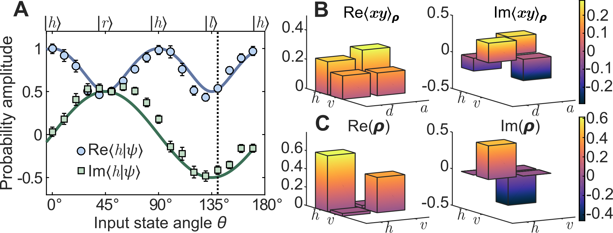
A joint measurement on twins of can reveal correlations between complementary properties in . We measure the entire joint quasiprobability distribution for the complementary polarization observables using diagonal and anti-diagonal projectors, and using horizontal and vertical projectors. This is repeated for a variety of different input states . For the input state indicated by the dashed line in Fig. 3A, correlations can be seen in , as shown in Fig. 3B. With the ability to exhibit correlations, is now a complete description of the quantum state [32]. In particular, the wave function of the state (see Fig. 3A) is any cross-section of . Moreover, the density matrix (see Fig. 3C) can be obtained with a Fourier transform of . This is the key experimental result. In the classical world, simultaneously measuring complementary properties gives the system’s state. This result demonstrates that simultaneously measuring complementary observables on twins, similarly, gives the system’s state.
In addition to its fundamental importance, our result has potential practical advantages as a state determination procedure. It is valid for higher dimensional states [32] for which standard quantum tomography requires prohibitively many measurements. Specifically, a -dimensional state typically requires measurements in bases to be reconstructed tomographically. In contrast, here the wave function is obtained directly (i.e. without a reconstruction algorithm) from experimental measurements of only two observables, and .
Our results uncover striking connections with other joint measurement techniques, despite the physics of each approach being substantially different. For example, the joint quasiprobability is also the average outcome of another joint measurement strategy: the weak measurement of followed by a measurement of on a single system [16, 15, 19]. Furthermore, in the continuous-variable analogue of our work, measurements of complementary observables on cloned Gaussian states [38] give a different, but related, quasiprobability distribution for the quantum state known as the Q-function [10]. Finally, the result of a joint measurement on phase-conjugated Gaussian states can be used in a feedforward to produce optimal clones [39]. These connections emphasize the central role of optimal cloning in quantum mechanics [23, 27] and clarify the intimate relation between joint measurements of complementary observables and determining quantum states [4, 6].
We anticipate that simultaneous measurements of non-commuting observables can be naturally implemented in quantum computers using our technique, since the operation can be achieved using a controlled-SWAP quantum logic gate [19, 40]. As joint measurements are pivotal in quantum mechanics, this will have broad implications for state estimation [13, 14, 15, 16], quantum control [17], and quantum foundations [18, 12]. For instance, we anticipate that our method can be used to efficiently and directly measure high-dimensional quantum states that are needed for fault-tolerant quantum computing and quantum cryptography [36].
Acknowledgements.
This work was supported by the Canada Research Chairs (CRC) Program, the Natural Sciences and Engineering Research Council (NSERC), and Excellence Research Chairs (CERC) Program.References
- [1] M. Ozawa, Phys. Lett. A 320, 367 (2004).
- [2] P. Busch, P. Lahti, and R. F. Werner, Rev. Mod. Phys. 86, 1261 (2014).
- [3] W. Heisenberg, Z. Phys. 43, 172 (1927).
- [4] E. Wigner, Phys. Rev. 40, 749 (1932).
- [5] E. Arthurs and J. L. Kelly, Bell Syst. Tech. J. 44, 725 (1965).
- [6] W. M. de Muynck, P. A. E. M. Janssen, and A. Santman, Found. Phys. 9, 71 (1979).
- [7] V. B. Braginsky, Y. I. Vorontsov, and K. S. Thorne, Science 209, 547 (1980).
- [8] C. Carmeli, T. Heinosaari, and A. Toigo, Phys. Rev. A 85, 012109 (2012).
- [9] J. Shapiro and S. Wagner, IEEE J. Quant. Electron. 20, 803 (1984).
- [10] U. Leonhardt and H. Paul, Phys. Rev. A 47, R2460 (1993).
- [11] G. Colangelo, F. M. Ciurana, L. C. Bianchet, R. J. Sewell, and M. W. Mitchell, Nature 543, 525 (2017).
- [12] M. Ringbauer, D. N. Biggerstaff, M. A. Broome, A. Fedrizzi, C. Branciard, and A. G. White, Phys. Rev. Lett. 112, 020401 (2014).
- [13] J. S. Lundeen, B. Sutherland, A. Patel, C. Stewart, and C. Bamber, Nature 474, 188 (2011).
- [14] G. S. Thekkadath, L. Giner, Y. Chalich, M. J. Horton, J. Banker, and J. S. Lundeen, Phys. Rev. Lett. 117, 120401 (2016).
- [15] C. Bamber and J. S. Lundeen, Phys. Rev. Lett. 112, 070405 (2014).
- [16] J. Z. Salvail, M. Agnew, A. S. Johnson, E. Bolduc, J. Leach, and R. W. Boyd, Nat. Photon. 7, 316 (2013).
- [17] S. Hacohen-Gourgy, L. S. Martin, E. Flurin, V. V. Ramasesh, K. B. Whaley, and I. Siddiqi, Nature 538, 491 (2016).
- [18] L. A. Rozema, A. Darabi, D. H. Mahler, A. Hayat, Y. Soudagar, and A. M. Steinberg, Phys. Rev. Lett. 109, 100404 (2012).
- [19] H. F. Hofmann, Phys. Rev. Lett. 109, 020408 (2012).
- [20] A. Černoch, J. Soubusta, L. Bartůšková, M. Dušek, and J. Fiurášek, Phys. Rev. Lett. 100, 180501 (2008).
- [21] As is usual for a probability, is estimated from repeated trials using an identical ensemble of input systems. This is implicit for probabilities and expectation values throughout the paper.
- [22] The strategy considered here is informationally equivalent to separating an identical ensemble into two and measuring with one half and with the other half. Knowing only these two marginal distributions is insufficient to determine the quantum state [42].
- [23] W. K. Wootters and W. H. Zurek, Nature 299, 802 (1982).
- [24] V. Scarani, S. Iblisdir, N. Gisin, and A. Acín, Rev. Mod. Phys. 77, 1225 (2005).
- [25] V. Bužek and M. Hillery, Phys. Rev. A 54, 1844 (1996).
- [26] N. Gisin and S. Massar, Phys. Rev. Lett. 79, 2153 (1997).
- [27] D. Bruss, A. Ekert, and C. Macchiavello, Phys. Rev. Lett. 81, 2598 (1998).
- [28] J. Niset, A. Acín, U. L. Andersen, N. Cerf, R. García-Patrón, M. Navascués, and M. Sabuncu, Phys. Rev. Lett. 98, 260404 (2007).
- [29] S. Massar and S. Popescu, Phys. Rev. Lett. 74, 1259 (1995).
- [30] G. M. D’Ariano, C. Macchiavello, and M. F. Sacchi, J. Opt. B: Quantum Semiclass. Opt. 3, 44 (2001).
- [31] T. Brougham, E. Andersson, and S. M. Barnett, Phys. Rev. A 73, 062319 (2006).
- [32] See supplementary materials for details on the experimental setup, derivations, and some additional data. It also includes Ref. [41].
- [33] R. A. Campos and C. C. Gerry, Phys. Rev. A 72, 065803 (2005).
- [34] W. T. M. Irvine, A. Lamas Linares, M. J. A. de Dood, and D. Bouwmeester, Phys. Rev. Lett. 92, 047902 (2004).
- [35] E. Nagali, L. Sansoni, F. Sciarrino, F. De Martini, L. Marrucci, B. Piccirillo, E. Karimi, and E. Santamato, Nat. Photon. 3, 720 (2009).
- [36] F. Bouchard, R. Fickler, R. W. Boyd, and E. Karimi, Science Adv. 3 (2017), 10.1126/sciadv.1601915.
- [37] J.-P. W. MacLean, K. Ried, R. W. Spekkens, and K. J. Resch, “Quantum-coherent mixtures of causal relations,” (2016), arXiv:1606.04523 .
- [38] U. L. Andersen, V. Josse, and G. Leuchs, Phys. Rev. Lett. 94, 240503 (2005).
- [39] M. Sabuncu, U. L. Andersen, and G. Leuchs, Phys. Rev. Lett. 98, 170503 (2007).
- [40] R. B. Patel, J. Ho, F. Ferreyrol, T. C. Ralph, and G. J. Pryde, Science Adv. 2 (2016), 10.1126/sciadv.1501531.
- [41] T. Durt, B.-G. Englert, I. Bengtsson, and K. Życzkowski, Int. J. Quantum Inform. 8, 535 (2010).
- [42] A. I. Lvovsky and M. G. Raymer, Rev. Mod. Phys. 81, 299 (2009).
Supplementary Material
Experimental Setup
A detailed figure containing the experimental setup is shown in Fig. S1. A 40 mW continuous-wave diode laser at 404 nm pumps a type-II -barium borate crystal. Through spontaneous parametric down-conversion, pairs of 808 nm photons with orthogonal polarization are generated collinearly with the pump laser. The latter is then blocked by a long pass filter. The photon pair splits at a polarizing beam splitter (PBS), and each photon is coupled into a polarization-maintaining single mode fiber. The path length difference between the photon paths is adjusted with a delay stage. A spinning (2 Hz) half-wave plate produces a completely mixed state at one fiber output, while a half-wave plate and quarter-wave plate produce the state to be cloned at the other fiber output. A displaced Sagnac interferometer composed of two BS is used instead of the interferometer in Fig. 1 (of main text), since it is more robust to air fluctuations and other instabilities. The phase between red and blue paths is adjusted by slightly rotating one of the mirrors in the interferometer in order to change the path length difference between both paths. A series of wave plates and a PBS are used to implement the projectors and . Detectors are single photon counting silicon avalanche photodiodes. Using time-correlation electronics, we count coincidence events that occur in a 5 nanosecond window and average over 60 seconds for each measurement.
Joint measurement on optimal clones
For qudits, the -dimensional observables and are complementary if their eigenstates and all satisfy . We use the notation . The output of an optimal cloner for qudits is:
| (S4) |
with . Consider measuring in mode and in mode . As shown in Ref. [19], the joint probability of measuring outcome and is:
| (S5) | ||||
The terms and could be obtained from a joint measurement on trivial clones. In contrast, the last term is obtained from a joint measurement on twins, and is a joint quasiprobability of simultaneously measuring both and on . In order to isolate the latter term, we use the fact that the joint measurement contribution of the trivial clones does not depend on the phase , giving:
| (S6) |
When the input state is pure, that is , then , where . For some , the phase of is constant for all and so the wave function can be expressed in the basis of as . As usual, the constant is found by normalizing . Thus, using Eq. S6, any complex amplitude of the wave function can be found from:
| (S7) |
The choice of is equivalent to choosing a phase reference for the wave function. In Fig. 3A of the main text, we use , which defines the diagonal polarization as . We choose to make the normalization constant a real number, i.e. .
For mixed input states, the joint quasiprobability is related to the density matrix via a discrete Fourier transform (see derivation below).
Relating the joint quasiprobability to the density matrix
Here we summarize the connection between the joint quasiprobability distribution and the density matrix. Consider the -dimensional complementary observables and with eigenstates and such that for any . Without loss of generality [41], one can take the basis to be defined in terms of a discrete Fourier transform of : . This fixes a phase relation for the inner product of all the eigenstates of both bases:
| (S8) |
A general -dimensional quantum state can be written in the basis of as . We wish to relate the coefficients to the joint quasiprobability distribution described in the main text, i.e. . Recall that we use the notation . Thus takes the form of . Inserting the expanded form of :
| (S9) |
This shows that the joint quasiprobability is the discrete Fourier transform of the density matrix. The equation can be inverted by taking the inverse Fourier transform of both sides:
| (S10) |
In the case of polarization qubits, and . Then the equation relating the two density matrix and the joint quasiprobability is:
| (S11) |
Eq. S11 is used to calculate the density matrix in Fig. 3C of the main text.
Trivial to optimal clones
When the two input photons are temporally distinguishable, Hong-Ou-Mandel interference does not occur at the first beam splitter, and the cloner produces trivial clones . Conversely, for temporally indistinguishable photons, we produce . Photons that are partially distinguishable can be decomposed into the form
| (S12) |
where is a temporal distinguishability factor. In particular, the temporal mode of the delayed photon in mode can be written as where is the delay, while the other photon in mode is described by . For a Gaussian spectral amplitude where is the central frequency of the photons and is their spectral width, the distinguishability factor is given by
| (S13) |
In the experiment, we adjust the delay by moving the delay stage. The parameter is extracted from fitting a Gaussian to the Hong-Ou-Mandel dip (see Fig. S2).
Extended Data

