Magnetic Catalysis in Antiferromagnetic Films
Abstract
We study the low-temperature behavior of antiferromagnets in two spatial dimensions that are subjected to a magnetic field oriented perpendicular to the staggered magnetization order parameter. The evaluation of the partition function is carried to two-loop order within the systematic effective Lagrangian technique. Low-temperature series that are valid in weak magnetic and staggered fields are derived for the pressure, staggered magnetization, and magnetization. Remarkably, at =0, the staggered magnetization is enhanced by the magnetic field, implying that the phenomenon of magnetic catalysis also emerges in antiferromagnetic films.
1 Motivation
The thermodynamic properties of antiferromagnets in two spatial dimensions have been the topic of numerous studies. Within microscopic, phenomenological, and numerical approaches, the free energy density, staggered magnetization, and other observables have been explored extensively at low temperatures [1, 2, 3, 4, 5, 6, 7, 8, 9, 10, 11, 12, 13, 14, 15, 16, 17] – in particular also in magnetic fields [18, 19, 20, 21, 22, 23, 24, 25, 26, 27, 28, 29, 30, 31, 32, 33, 34, 35, 36, 37, 38, 39, 40, 41, 42, 43, 44, 45, 46, 47, 48, 49, 50, 51, 52]. Still, a fully systematic analysis of how a weak magnetic field, in presence of a weak staggered field, affects the low-energy physics of antiferromagnetic films – both at =0 and finite temperature – appears to be lacking.
Instead of relying on phenomenological or microscopic techniques such as modified spin-wave theory, the present analysis is based on the effective Lagrangian method that has the virtue of being fully systematic. The crucial point is that the relevant degrees of freedom in an antiferromagnet at low temperatures – the spin waves or magnons – are the Goldstone bosons of a spontaneously broken internal symmetry: .11 1 Strictly speaking, at finite temperature and in two spatial dimensions, spontaneous symmetry breaking does not occur because of the Mermin-Wagner theorem [53]. However, the low-temperature physics is still dominated by the spin waves and the staggered magnetization is different from zero at low and weak fields. In this sense the staggered magnetization is still referred to as order parameter in the present study. Goldstone boson effective field theory has been developed in the eighties in the context of quantum chromodynamics [54, 55], but the same universal principles can be applied to condensed matter systems [56, 57], where the phenomenon of spontaneous symmetry breaking is ubiquitous.
Within effective field theory, the thermodynamic properties of antiferromagnets in two spatial dimensions have been analyzed in Refs. [58, 59, 60, 61]. Some of these studies – apart from the inclusion of a staggered field – also consider the effect of an external magnetic field. However a systematic discussion of how the thermodynamic variables and the physics at =0 depend on these fields, has not yet been presented. In particular, the situation where the magnetic field is oriented perpendicular to the staggered field, has not been discussed on the effective level so far. This motivates the present work where we systematically investigate the impact of a perpendicular magnetic field onto the low-energy behavior of =2+1 antiferromagnets. We evaluate the partition function up to two-loop order, derive the low-temperature series for the free energy density, pressure, staggered magnetization, and magnetization, and also consider the behavior of the system at zero temperature.
In the absence of a magnetic field, the spin-wave interaction does not yet manifest itself: up to two-loop order, the low-temperature series just correspond to the free magnon gas. In nonzero magnetic fields, however, the spin-wave interaction leads to interesting effects. In the pressure -- irrespective of the strength of the magnetic and staggered field -- the interaction among the magnons is repulsive. Regarding the order parameter at finite temperature22 2 See footnote 1., we also observe subtle effects: if the temperature is raised from =0 to finite -- while keeping the strength of the staggered and magnetic field fixed -- the order parameter decreases as a consequence of the spin-wave interaction. Remarkably, at zero temperature, the staggered magnetization is enhanced in weak magnetic fields. This phenomenon -- magnetic catalysis -- has been observed in quantum chromodynamics, graphene, topological insulators, and other systems.33 3 As we comment in subsection 4.2, magnetic catalysis in antiferromagnetic films is different because no charged particles or Landau levels are involved. Finally, the perpendicular magnetic field – both at zero and finite temperature – causes the magnetization to take positive values, signaling that the spins get tilted into the magnetic field direction.
The article is organized as follows. The incorporation of the perpendicular magnetic field, along with some essential information on the effective Lagrangian method, is discussed in Sec. 2. The perturbative evaluation of the free energy density up to two-loop order is provided in Sec. 3. The low-temperature series for various thermodynamic quantities – pressure, staggered magnetization, and magnetization – in presence of weak staggered and magnetic fields, are derived in Sec. 4. The role of the spin-wave interaction in these observables is illustrated in various figures. In the same section we also consider the behavior at =0 and discuss the phenomenon of magnetic catalysis. Finally, in Sec. 5 we present our conclusions. Technical details on vertices with an odd number of magnon lines and the evaluation of a specific two-loop diagram can be found in two separate appendices.
2 Microscopic and Effective Description
Antiferromagnets in two spatial dimensions are described by the quantum Heisenberg model,
| (2.1) |
where the summation extends over all nearest neighbor spins on a bipartite lattice, and the exchange integral is negative. The Heisenberg Hamiltonian is invariant under global internal O(3) symmetry. The antiferromagnetic ground state, however, is only invariant under O(2). As a consequence of the spontaneously broken rotation symmetry, two spin-wave branches – or two magnon particles – emerge in the low-energy spectrum. If the O(3) symmetry is exact, the two degenerate spin-wave branches follow the dispersion law
| (2.2) |
with as spin-wave velocity. According to Goldstone’s theorem, both excitations obey
| (2.3) |
The symmetric model can be extended by incorporating a staggered field and a magnetic field ,
| (2.4) |
that both explicitly break O(3)-invariance. Now the spontaneously broken symmetry is only approximate: the spin-wave branches exhibit an energy gap, i.e., the magnons are no longer Goldstone bosons as they become massive. In particle physics it is common to call such excitations pseudo-Goldstone bosons.
Let us turn to the effective description of the =2+1 antiferromagnet in presence of staggered and magnetic fields. This situation has been discussed in detail in sections IX-XI of Ref. [62] (see also Ref. [56]). Here we merely list the relevant expressions. The basic low-energy degrees of freedom – the two antiferromagnetic magnon fields – we denote by , and collect them in a unit vector ,
| (2.5) |
The ground state of the antiferromagnet is represented by , and the magnons correspond to fluctuations in the orthogonal directions.
The low-energy effective theory is based on a systematic expansion in powers of momenta, i.e., on a derivative expansion of the effective Lagrangian. The leading term – – contains two space-time derivatives,
| (2.6) |
where the covariant derivative is
| (2.7) |
The magnetic field is incorporated through the time component of the covariant derivative . On the other hand, the staggered field couples to that represents the order parameter: the staggered magnetization at zero temperature, zero external fields, and infinite volume. Apart from , a second low-energy effective constant appears in : the quantity that is related to the spin stiffness (or helicity modulus) by . Note that the magnetic field counts as order like the time derivative, whereas the staggered field is of order .
The subleading piece in the effective Lagrangian is of order ,
| (2.8) | |||||
and contains five next-to-leading order (NLO) effective constants whose numerical values have to be determined or estimated to make the effective field theory predictive (see below).
We now comment on an important issue related to Lorentz-invariance. The leading and next-to-leading effective Lagrangians are Lorentz-invariant. In view of the fact that the underlying bipartite lattices are not even space-rotation invariant, why is our approach legitimate? The first observation is that the leading piece is strictly (pseudo-)Lorentz-invariant, the spin-wave velocity taking the role of the speed of light. This accidental symmetry emerges because lattice anisotropies only show up at order (and beyond) in the effective Lagrangian [59]. On the other hand, in one should include all additional terms that are permitted by the lattice geometry. However, as we explain below, these effects only start manifesting themselves at next-to-next-to leading order in the low-temperature expansion which is beyond two-loop accuracy we pursue in the present evaluation. This perfectly justifies maintaining a (pseudo-)Lorentz-invariant structure also in .
In the following we consider the scenario where the magnetic field points into a direction perpendicular to the staggered field,
| (2.9) |
While we have chosen to point into the 1-direction, the physics would be the same had we chosen the 2-direction. Note that the staggered field points into the 0-direction, aligned with the staggered magnetization order parameter or ground state .
The leading-order effective Lagrangian gives rise to the following magnon dispersion relations,
| (2.10) |
These results coincide with the expressions derived within microscopic or phenomenological descriptions – see, e.g., Refs. [63, 64]. Remarkably, one of the magnons is not affected by the magnetic field. The structure of the dispersion relation is relativistic in both cases, and the corresponding ”magnon mass terms” are identified as
| (2.11) |
Note that the staggered field emerges linearly while the dependence on the magnetic field is quadratic. If the fields are switched off, we reproduce the linear and ungapped dispersion relation Eq. (2.2).44 4 We have set the spin-wave velocity to one.
It is convenient to utilize dimensional regularization in the perturbative evaluation of the partition function. The zero-temperature propagators for antiferromagnetic magnons, in presence of and , amount to
| (2.12) |
where and are defined in Eq. (2.11). The corresponding thermal propagators in Euclidean space are given by
| (2.13) |
We emphasize that the magnetic and staggered field are treated as perturbations that explicitly break O(3) invariance of the Heisenberg Hamiltonian. As long as these fields are weak, the O(3) symmetry still is approximate, and our basic setting is valid: it is conceptually consistent to start from the collinear antiferromagnetic ground state and interpret the two magnons as oscillations of the staggered magnetization order parameter. It is well-known, however, that in presence of magnetic fields perpendicular to the staggered magnetization, the spins get tilted, creating a canted (non-collinear) phase (see, e.g., Refs. [23, 43, 49]). If the canting angle is large, the magnetic field can no longer be considered as a small perturbation. Rather the canted phase should be chosen as the starting configuration underlying the perturbative expansion. Most importantly, since the spontaneous symmetry breaking pattern then is O(3) 1, not two, but three Goldstone fields emerge in the low-energy spectrum. This scenario, i.e., the low-temperature physics of canted phases, we postpone for future studies – in the present investigation we consider weak magnetic fields where only two spin-wave branches are relevant.
3 Evaluation of the Partition Function

We now evaluate the partition function for the =2+1 antiferromagnet subjected to the magnetic and staggered fields defined in Eq. (2.9). The relevant Feynman diagrams up to two-loop order are shown in Fig. 1.55 5 The perturbative evaluation of the partition function is described in more detail in section 2 of Ref. [60] and in appendix A of Ref. [65]. Regarding the effective Lagrangian technique in general, the interested reader may consult Refs. [66, 67, 68]. The crucial point is that we are dealing with a systematic low-temperature expansion of the partition function where each magnon loop is suppressed by one power of temperature. The free Bose gas contribution is given by the one-loop graph (order ), while the two-loop graph is of order .
The incorporation of a perpendicular magnetic field generates extra vertices that involve an odd number of magnon lines. With respect to , the explicit terms are proportional to one time derivative and read
| (3.1) |
These contributions, along with those originating from , create vertices with magnon lines: in presence of a perpendicular magnetic field, the set of Feynman diagrams has to be extended by the graphs depicted in Fig. 2. Note that in the diagrams depicted in Fig. 1, the magnetic field manifests itself implicitly in the thermal propagator through .

The tree graphs and merely contribute to the energy density at zero temperature,
| (3.2) |
The dominant temperature-dependent contribution comes from one-loop graph ,
| (3.3) | |||||
Note that the Gamma function is finite in two spatial dimensions,
| (3.4) |
The quantities and are the kinematical functions related to the free magnon gas,
| (3.5) |
Next, the two-loop graph contributes with
| (3.6) | |||||
where are the thermal propagators evaluated at the origin,
| (3.7) |
In the absence of the magnetic field, we have , such that the entire two-loop contribution vanishes.
Finally, the explicit evaluation of diagram yields zero,
| (3.8) |
while the sunset diagram amounts to
| (3.9) |
This integral over the torus , with circle defined as , is divergent in the ultraviolet. The renormalization of this expression and the evaluation of the thermal sums is described in appendix B. The finite contribution to the free energy density is given by
| (3.10) |
The dimensionless function is defined in Eq. (B.14), and the dimensionless parameters and are
| (3.11) |
A plot of is provided in Fig. 3.
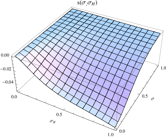
Remarkably, up to two-loop order, the NLO effective constants only show up in the tree graph . These constants – that are a priori unknown – hence only matter in temperature-independent contributions. The low-temperature expansion, in particular the impact of the spin-wave interaction, is governed by the leading effective Lagrangian . Up to two-loop order, the thermal properties of the =2+1 antiferromagnet are thus rigorously captured by our effective field theory approach that is based on (pseudo-)Lorentz invariance. The specific geometry of the underlying bipartite lattice is irrelevant as far as the structure of the low-temperature expansion is concerned. Alternatively, this can be seen as follows. Lattice anisotropies modify the dispersion relation
| (3.12) |
at order – the specific terms and coefficients indeed depend on the lattice geometry. While the linear term in the dispersion relation yields the dominant contribution of order in the free energy density, the corrections contribute at order which is beyond our scope. Therefore our (pseudo-)Lorentz-invariant framework is perfectly legitimate: we make no mistake by merely considering the leading term in the dispersion relation.
The lattice structure only reflects itself in the numerical values of the leading-order effective constants and that have been determined with high-precision loop-cluster algorithms. For the square lattice [69] they read
| (3.13) |
for the honeycomb lattice [70] they are
| (3.14) |
with
| (3.15) |
Note that the spin stiffness as well as , much like the spin-wave velocity , are given in units of (exchange integral) and (lattice size).
4 Low-Temperature Series
The low-temperature physics of the system can be captured by various dimensionless ratios. As independent quantities we define the parameters and as
| (4.1) |
For the effective low-energy expansion to be consistent, the temperature as well as the staggered and magnetic field must be small compared to the scale that characterizes the microscopic system. The natural scale in the Heisenberg antiferromagnet is the exchange integral . In the present study, we define low temperatures and weak fields by
| (4.2) |
The factors in Eq. (4.1) were introduced in analogy to the relevant scale in quantum chromodynamics (see Ref. [60]). The point is that for the antiferromagnet – both on the square and honeycomb lattice – the denominator is of the order of . The parameters hence measure temperature and field strength relative to the underlying microscopic scale.
Whereas temperature and magnetic field can be arbitrarily small, it should be noted that the staggered field can not be switched off. This is a consequence of the Mermin-Wagner theorem [53] and the fact that the staggered magnetization – unlike the magnetization – represents the order parameter. As we have discussed on previous occasions, the domain where the effective expansion fails due to the smallness of the staggered field, is tiny. The interested reader is referred to Figs. 2 and 3 of Ref. [61].
4.1 Pressure
We first discuss the pressure, defined by
| (4.3) |
The quantity includes all terms in the energy density that do not depend on temperature. Introducing dimensionless functions as
| (4.4) |
the structure of the low-temperature series becomes more transparent because powers of temperature are explicit. For the pressure we get
| (4.5) |


The dominant term of order (graph ) corresponds to the free Bose gas. The term of order (graphs and ) represents the leading interaction contribution. In the absence of a perpendicular magnetic field, the spin-wave interaction does not manifest itself at two-loop order: the corresponding coefficient is zero. On the other hand, if a perpendicular magnetic field is present, the behavior of the system is quite interesting: in Fig. 4 we depict the ratio
| (4.6) |
that measures strength and sign of the spin-wave interaction in the pressure relative to the free Bose gas contribution. The plots refer to the temperatures (left) and (right). As the figure suggests, irrespective of the strength of the magnetic and staggered field, the interaction among antiferromagnetic magnons is repulsive.66 6 It has been argued previously that the limit becomes problematic in any thermodynamical observable. However, according to Ref. [61], the error introduced in the pressure is tiny and not visible in Fig. 4 of the present work.
4.2 Staggered Magnetization
The staggered magnetization order parameter can be extracted from the free energy density by
| (4.7) |
The low-temperature series takes the structure77 7 We do not display the coefficient since the expression is rather lengthy – it can trivially be obtained from given in Sec. 3.
| (4.8) |
The spin-wave interaction comes into play at order . Again, in zero magnetic field, there is no interaction term at two-loop order: .


To explore the impact of the spin-wave interaction in the order parameter, we consider the ratio
| (4.9) |
that we depict in Fig. 5 for the temperatures . The quantity is negative in the parameter region we consider. Negative means that if the temperature is raised from =0 to finite – while keeping and fixed – the order parameter decreases due to the spin-wave interaction.
Recall that it makes no sense to address the two-dimensional system in very weak staggered fields within our framework, because the effective expansion breaks down when one approaches the limit .88 8 A detailed discussion of how this relates to the Mermin-Wagner theorem, can be found at the end of section 4 in Ref. [71]. In our plots we have chosen the staggered field strength as
| (4.10) |
This guarantees that the effects we observe are indeed physical and not just artifacts of our effective calculation extrapolated to a forbidden parameter region.
At zero temperature, the order parameter is given by
| (4.11) | |||||
In contrast to finite temperature, at =0, next-to-leading order effective constants arise in the low-energy expansion of the staggered magnetization. The actual values of these constants depend on the underlying system and are not fixed by the symmetries. They should be determined by numerical simulations, comparison with microscopic calculations, or through experiments. Unfortunately, in the case of the =2+1 antiferromagnet, none of these options seems to be available.99 9 The exception is Ref. [69] where the combination of NLO effective constants was determined using a loop-cluster algorithm. Still, their magnitude can be estimated. According to Ref. [72] they are very small, of order
| (4.12) |
much like the other NLO effective constants and . It should be noted that the above estimate concerns their magnitude, but leaves open their signs. However these corrections are small – moreover, the dominant contributions in the series (4.11) do not involve NLO effective constants.
At =0 and in zero magnetic field, the series is characterized by powers of ,
| (4.13) |
and in zero staggered field1010 10 It is perfectly legitimate at =0 to consider the limit . Only at finite it is inconsistent to switch off the staggered field in our effective field theory approach. by powers of ,
| (4.14) |
While the order parameter is indeed expected to increase when the staggered field becomes stronger, the behavior with respect to the magnetic field comes rather unexpectedly: in the series (4.14), the term linear in is small, but positive. The order parameter thus increases when a weak perpendicular magnetic field is applied. Notice that the subleading correction (order ) involves the NLO effective constant whose sign remains open. Still, the behavior of the order parameter in weak magnetic fields is dominated by the leading term that is strictly positive. We emphasize that this result is universal in the sense that the term of order is the same for any bipartite lattice: the only difference between, e.g., the square and honeycomb lattice, concerns the actual values of the effective constants and .
The phenomenon that the order parameter is enhanced by an external magnetic field when the order parameter is already present in zero magnetic field, is called magnetic catalysis according to Ref. [73]. It has been observed in quantum chromodynamics, where the quark condensate – the order parameter of the spontaneously broken chiral symmetry – increases at =0 in presence of a magnetic field [74, 75, 76, 73]. Magnetic catalysis has also been reported in condensed matter systems like graphene [77] and three-dimensional topological insulators [78]. The fact that the staggered magnetization is enhanced at =0 in square lattice antiferromagnets subjected to a magnetic field perpendicular to the order parameter, has been reported in Ref. [46].
It should be pointed out that the phenomenon of magnetic catalysis – as it is discussed in the context of QCD or, e.g., graphene – involves charged particles and Landau levels. The mechanism of magnetic catalysis is thus rather subtle and different from the mechanism leading to magnetic catalysis in =2+1 antiferromagnets where no charged particles are involved in its low-energy description. The fact that the staggered magnetization grows in presence of a weak perpendicular magnetic field, is simply due to the suppression of quantum fluctuations of the order parameter vector by the magnetic field. Still, according to the definition given in Ref. [73], we are dealing with magnetic catalysis.
4.3 Magnetization
The low-temperature expansion of the magnetization,
| (4.15) |
takes the form1111 11 The coefficient can trivially be obtained from given in Sec. 3.
| (4.16) |
The free Bose gas contribution is proportional to one power of temperature, while the spin-wave interaction is contained in the -term.


In Fig. 6, for the temperatures , we plot the total temperature-dependent part of the magnetization
| (4.17) |
The quantity is negative in the entire parameter domain we consider. Negative means that the magnetization decreases when we go from from =0 to finite while keeping and fixed. This is what one would expect.


Remarkably, the quantity
| (4.18) |
that only takes into account the spin-wave interaction part, is positive as we illustrate in Fig. 7 that refers to the temperatures . Positive means that if the temperature is raised from =0 to finite – while keeping and fixed – the magnetization grows due to the spin-wave interaction. This result appears to be rather counterintuitive. But it is important to point out that we are dealing with weak effects originating from the spin-wave interaction. The dominant behavior at finite temperature is given by the free Bose gas term. Indeed, the total temperature-dependent magnetization (not just the interaction part), is strictly negative according to Fig. 6.
Finally, at zero temperature, the magnetization amounts to
| (4.19) | |||||
Again, NLO effective constants – – show up in subleading corrections. If the magnetic field is switched off, the magnetization tends to zero as it should,
| (4.20) |
In the limit , the expansion in the magnetic field involves integer powers of ,
| (4.21) |
The leading contributions are positive, whereas the sign of -term remains open. The leading terms, however, do not involve NLO effective constants, such that the magnetization takes positive values in presence of the magnetic field. As one would expect, the magnetization in the direction of the magnetic field no longer is zero, since the spins get tilted.
5 Conclusions
We have considered the low-energy properties of antiferromagnetic films subjected to magnetic fields perpendicular to the staggered magnetization order parameter. Within effective field theory we have systematically derived the low-temperature expansions for the free energy density, pressure, order parameter, and magnetization.
In presence of a weak magnetic field, the spin-wave interaction in the pressure is repulsive, irrespective of the strength of the magnetic and staggered field. The order parameter decreases due to the spin-wave interaction, when the temperature is raised from =0 to finite – while keeping and fixed. Finally, the magnetization – both at zero and finite temperature – takes positive values: the spins get tilted into the direction of the external perpendicular magnetic field.
At zero temperature, both the magnetization and staggered magnetization grow when a perpendicular magnetic field is applied. While this behavior is expected for the magnetization, the enhancement of the order parameter in presence of the magnetic field comes rather unexpectedly. It implies that the phenomenon of magnetic catalysis – well-known in quantum chromodynamics, graphene and other condensed matter systems – also emerges in antiferromagnetic films.
Acknowledgments
The author thanks J. O. Andersen, A. Auerbach, T. Brauner, H. Leutwyler, I. A. Shovkovy and R. R. P. Singh for correspondence.
Appendix A Vertices with an Odd Number of Magnon Lines
Magnetic fields perpendicular to the staggered magnetization order parameter give rise to vertices that involve an odd number of magnon lines. Explicitly, vertices with one magnon line originate from
| (A.1) |
while vertices with three magnon lines are generated by
| (A.2) |
Note that we only consider contributions from and – higher-order pieces of the effective Lagrangian also yield such vertices, but they do not contribute up to order in the partition function, as we argue below. The additional Feynman diagrams that can be constructed from the expressions (A.1) and (A.2) are depicted in Fig. 2. According to (A.1), the line emitted (or absorbed) by a one-magnon vertex always corresponds to . In case of a three-magnon vertex, according to (A.2), we either have or – in particular, three magnons of the same type are never emitted or absorbed simultaneously.
An important observation that drastically reduces the number of additional Feynman graphs, is that the one-magnon vertices from and are irrelevant. In the evaluation of the partition function they lead to integrals of the form
| (A.3) |
where is the Euclidean time derivative corresponding to the coordinate . The function , depending on the topology of the diagram, may contain an arbitrary number of propagators that involve additional time and space derivatives. But the point is that – irrespective of the complexity of the diagram – the integration over the coordinates of the first vertex, i.e., integration over the coordinates of the one-magnon vertex, is identically zero. One concludes that the relevant new diagrams must involve vertices with at least three magnon lines.
This then leads to the two-loop diagrams and of Fig. 2. Any other diagram that involves vertices with an odd number of magnon lines is at least of order , i.e., beyond the scope of the present study. Remarkably, the explicit evaluation of diagram yields zero,
| (A.4) |
while the sunset diagram contributes with
| (A.5) |
This integral over the torus , with circle defined as , is divergent in the ultraviolet. In the subsequent appendix we show how to isolate the singularities and how to evaluate the finite pieces.
Appendix B Evaluation of the Sunset Diagram
In order to process the integral (A.5), we decompose the thermal propagators as
| (B.1) |
where the are the zero-temperature propagators defined in Eq. (2.12). The integral then takes the form
| (B.2) |
The first four integrals over the torus are convergent in . The four remaining integrals that involve two or three zero-temperature propagators, however, are singular in the limit , and need to be considered in detail. Following Ref. [79], we cut out a sphere of radius around the origin and write the respective integrals over the torus as
| (B.3) |
The evaluation of the integrals over the complement of the torus poses no problems in =3. In the integral over the sphere in line three, we subtract the piece ,
| (B.4) |
while in the integrals over the sphere in lines one and two, we perform the subtractions
| (B.5) |
Making use of
| (B.6) |
we end up with
| (B.7) |
The subtracted integrals over the sphere on the RHS are convergent in . The second integrals on the RHS we decompose further as
| (B.8) |
The integrals over the complement are well-defined. The integrals over all Euclidean space are finite in dimensional regularization in the limit ,
| (B.9) |
Finally, the last integral in Eq. (B.2) that contains three zero-temperature propagators, is decomposed as
| (B.10) |
The integrals over and are finite, but the integral over all Euclidean space is singular in . The corresponding counterterm ,
| (B.11) |
can be absorbed by NLO effective constants in , Eq. (3.2).
In conclusion, the first four integrals in the sunset contribution, Eq. (B.2), are well-defined and can be evaluated numerically in a straightforward manner, using the fact that the integrals are two-dimensional,
| (B.12) |
The evaluation of the remaining four integrals in Eq. (B.2) is more subtle, but can be handled within dimensional regularization using the method established in Ref. [79]. In the limit , the final – and finite – representation for the free energy density originating from the sunset diagram reads
| (B.13) | |||||
In a last step we collect all the above contributions in the dimensionless function ,
| (B.14) |
where the dimensionless ratios and are defined as
| (B.15) |
A plot of is provided in Fig. 3. Note the final result for the function must be independent of the size of the sphere which is an academic invention. We have verified that different sizes of the sphere indeed lead to the same .
References
- [1] S. Chakravarty, B. I. Halperin, and D. R. Nelson, Phys. Rev. Lett. 60, 1057 (1988).
- [2] D. P. Arovas and A. Auerbach, Phys. Rev. B 38, 316 (1988).
- [3] A. Auerbach and D. P. Arovas, Phys. Rev. Lett. 61, 617 (1988).
- [4] S. Chakravarty, B. I. Halperin, and D. R. Nelson, Phys. Rev. B 39, 2344 (1989).
- [5] M. Takahashi, Phys. Rev. B 40, 2494 (1989).
- [6] G. Gomez-Santos, J. D. Joannopoulos, and J. W. Negele, Phys. Rev. B 39, 4435 (1989).
- [7] T. Barnes, Int. J. Mod. Phys. C 2, 659 (1991).
- [8] E. Manousakis, Rev. Mod. Phys. 63, 1 (1991).
- [9] A. V. Chubukov, S. Sachdev, and J. Ye, Phys. Rev. B 49, 11919 (1994).
- [10] U.-J. Wiese and H.-P. Ying, Z. Phys. B 93, 147 (1994).
- [11] A. W. Sandvik, Phys. Rev. B 56, 11678 (1997).
- [12] A. Cuccoli, V. Tognetti, R. Vaia, and P. Verrucchi, Phys. Rev. B 56, 14456 (1997).
- [13] B. B. Beard, R. J. Birgeneau, M. Greven, and U.-J. Wiese, Phys. Rev. Lett. 80, 1742 (1998).
- [14] J.-K. Kim and M. Troyer, Phys. Rev. Lett. 80, 2705 (1998).
- [15] B.-G. Liu, Phys. Lett. A 259, 308 (1999).
- [16] E. C. Marino and M. B. Silva Neto, Phys. Rev. B 62, 142 (2000).
- [17] A. Sherman and M. Schreiber, Phys. Rev. B 63, 214421 (2001).
- [18] A. F. M. Arts, C. M. J. van Uijen, and H. W. de Wijn, Phys. Rev. B 15, 4360 (1977).
- [19] K. Fabricius, M. Karbach, U. Löw, and K.-H. Mütter, Phys. Rev. B 45, 5315 (1992).
- [20] S. Gluzman, Z. Phys. B 90, 313 (1993).
- [21] C. Millán and D. Gottlieb, Phys. Rev. B 50, 242 (1994).
- [22] S. Sachdev, T. Senthil, and R. Shankar, Phys. Rev. B 50, 258 (1994).
- [23] M.-W. Wu, T. Li, and H.-S. Wu, J. Phys.: Condens. Matter 6, 6535 (1994).
- [24] M. E. Zhitomirsky and T. Nikuni, Phys. Rev. B 57, 5013 (1998).
- [25] M. E. Zhitomirsky and T. Nikuni, Physica B 241-243, 573 (1998).
- [26] A. W. Sandvik, Phys. Rev. B 59, R14157 (1999).
- [27] M. E. Zhitomirsky and A. L. Chernyshev, Phys. Rev. Lett. 82, 4536 (1999).
- [28] A. V. Syromyatnikov and S. V. Maleyev, Phys. Rev. B 65, 012401 (2001).
- [29] T. Sommer, M. Vojta, and K. W. Becker, Eur. Phys. J. B 23, 329 (2001).
- [30] A. Honecker, Can. J. Phys. 79, 1557 (2001).
- [31] S. Yunoki, Phys. Rev. B 65, 092402 (2002).
- [32] O. F. Syljuasen and A. W. Sandvik, Phys. Rev. E 66, 046701 (2002).
- [33] A. Honecker, J. Schulenburg, and J. Richter, J. Phys.: Condens. Matter 16, S749 (2004).
- [34] M. Y. Veillette, J. T. Chalker, and R. Coldea, Phys. Rev. B 71, 214426 (2005).
- [35] A. L. Chernyshev, Phys. Rev. B 72, 174414 (2005).
- [36] I. Spremo, F. Schütz, P. Kopietz, V. Pashchenko, B. Wolf, M. Lang, J. W. Bats, C. Hu, and M. U. Schmidt, Phys. Rev. B 72, 174429 (2005).
- [37] P. J. Jensen, K. H. Bennemann, D. K. Morr, and H. Dreyssé, Phys. Rev. B 73, 144405 (2006).
- [38] A. Honecker and S. Wessel, Physica B 378-380, 1098 (2006).
- [39] N. Hasselmann, F. Schütz, I. Spremo, and P. Kopietz, C. R. Chimie 10, 60 (2007).
- [40] D. Yamamoto and S. Kurihara, Phys. Rev. B 75, 134520 (2007).
- [41] A. Kreisel, N. Hasselmann, and P. Kopietz, Phys. Rev. Lett. 98, 067203 (2007).
- [42] P. Thalmeier, M. E. Zhitomirsky, B. Schmidt, and N. Shannon, Phys. Rev. B 77, 104441 (2008).
- [43] A. Kreisel, F. Sauli, N. Hasselmann, and P. Kopietz, Phys. Rev. B 78, 035127 (2008).
- [44] O. F. Syljuasen, Phys. Rev. B 78, 180413 (2008).
- [45] A. L. Chernyshev and M. E. Zhitomirsky, Phys. Rev. B 79, 174402 (2009).
- [46] A. Lüscher and A. M. Läuchli, Phys. Rev. B 79, 195102 (2009).
- [47] D. J. J. Farnell, R. Zinke, J. Schulenburg, and J. Richter, J. Phys.: Condens. Matter 21, 406002 (2009).
- [48] C. J. Hamer, O. Rojas, and J. Oitmaa, Phys. Rev. B 81, 214424 (2010).
- [49] M. Mourigal, M. E. Zhitomirsky, and A. L. Chernyshev, Phys. Rev. B 82, 144402 (2010).
- [50] M. Siahatgar, B. Schmidt, and P. Thalmeier, Phys. Rev. B 84, 064431 (2011).
- [51] B. Schmidt, M. Siahatgar, and P. Thalmeier, J. Korean Phys. Soc. 62, 1499 (2013).
- [52] G. Palma and A. Riveros, Condens. Matter Phys. 18, 23002 (2015).
- [53] N. D. Mermin and H. Wagner, Phys. Rev. Lett. 17, 1133 (1966).
- [54] J. Gasser and H. Leutwyler, Ann. Phys. (N.Y.) 158, 142 (1984).
- [55] J. Gasser and H. Leutwyler, Nucl. Phys. B 250, 465 (1985).
- [56] H. Leutwyler, Phys. Rev. D 49, 3033 (1994).
- [57] J. O. Andersen, T. Brauner, C. P. Hofmann, and A. Vuorinen, JHEP 1408, 088 (2014).
- [58] P. Hasenfratz and H. Leutwyler, Nucl. Phys. B 343, 241 (1990).
- [59] P. Hasenfratz and F. Niedermayer, Z. Phys. B 92, 91 (1993).
- [60] C. P. Hofmann, Phys. Rev. B 81, 014416 (2010).
- [61] C. P. Hofmann, Nucl. Phys. B 904, 348 (2016).
- [62] C. P. Hofmann, Phys. Rev. B 60, 388 (1999).
- [63] M. I. Kaganov and V. M. Tsukernik, Sov. Phys. JETP 34, 1107 (1958).
- [64] A. I. Akhiezer, V. G. Baryakhtar, and M. I. Kaganov, Sov. Phys. Usp. 3, 567 (1961).
- [65] C. P. Hofmann, Phys. Rev. B 84, 064414 (2011).
- [66] H. Leutwyler, in Hadron Physics 94 – Topics on the Structure and Interaction of Hadronic Systems, edited by V. E. Herscovitz, C. A. Z. Vasconcellos, and E. Ferreira (World Scientific, Singapore, 1995), p. 1.
- [67] S. Scherer, Adv. Nucl. Phys. 27, 277 (2003).
- [68] T. Brauner, Symmetry 2, 609 (2010).
- [69] U. Gerber, C. P. Hofmann, F.-J. Jiang, M. Nyfeler, and U.-J. Wiese, J. Stat. Mech.: Theory Exp. (2009) P03021.
- [70] F.-J. Jiang, F. Kämpfer, M. Nyfeler, and U.-J. Wiese, Phys. Rev. B 78, 214406 (2008).
- [71] C. P. Hofmann, J. Stat. Mech.: Theory Exp. (2014) P02006.
- [72] B. Gavela, E. E. Jenkins, A. V. Manohar, and L. Merlo, Eur. Phys. J. C 76, 485 (2016).
- [73] J. O. Andersen, W. R. Naylor, and A. Tranberg, Rev. Mod. Phys. 88, 025001 (2016).
- [74] I. A. Shushpanov and A. V. Smilga, Phys. Lett. B 402, 351 (1997).
- [75] V. A. Miransky and I. A. Shovkovy, Phys. Rept. 576, 1 (2015).
- [76] S. Ozaki, Phys. Rev. D 89, 054022 (2014).
- [77] I. A. Shovkovy, Lect. Notes Phys. 871, 13 (2013).
- [78] E. V. Gorbar, V. A. Miransky, I. A. Shovkovy, and P. O. Sukhachov, Phys. Rev. B 94, 115429 (2016).
- [79] P. Gerber and H. Leutwyler, Nucl. Phys. B 321, 387 (1989).