Iterative Block Tensor Singular Value Thresholding for Extraction of Low Rank Component of Image Data

The high-dimensional data, also referred to as tensors, arise naturally in a number of scenarios, including image and video processing, and data mining [1]. However, most of the current processing techniques are developed for two-dimensional data [2]. The principal component analysis (PCA) is one of the most widely used one in two-dimensional data analysis [3].

The robust PCA (RPCA), as an extension of PCA, is an effective method in matrix decomposition problems [4]. Suppose we have a matrix $\bm{X}\in\mathbb{R}^{n_{1}\times n_{2}}$ , which can be decomposed as $\bm{X=L_{0}+S_{0}}$, where $\bm{L_{0}}$ is the low rank component of the matrix and $\bm{S_{0}}$ is the sparse component. The RPCA method has been applied to image alignment [5], surveillance video processing [6], illumination normalization for face images [7]. In most applications, the RPCA method should flatten or vectorize the tensor data so as to solve the problem in the matrix. It doesn’t use the structural feature of the data effectively since the information loss involves in the operation of matricization.

Tensor robust principal component analysis (TRPCA) has been studied in [8, 9] based on the tensor singular value decomposition (t-SVD). The advantage of t-SVD over the existing methods such as canonical polyadic decomposition (CPD) [10] and Tucker decomposition [11] is that the resulting analysis is very close to that of matrix analysis [12]. Similarly, suppose we are given a tensor $\mathcal{X}\in\mathbb{R}^{n_{1}\times n_{2}\times n_{3}}$ and it can be decomposed into low rank component and sparse component. We can write it as

where $\mathcal{L}_{0}$ denotes the low rank component, and $\mathcal{S}_{0}$ is the sparse component of the tensor. Fig. 1 is the illustration for TRPCA. In [8] the problem (1) is transformed to the convex optimization model:

where $\lVert\mathcal{L}_{0}\rVert_{*}$ is the tensor nuclear norm (see section 2 for the definition), $\lVert\mathcal{S}_{0}\rVert_{1}$ denotes the $\ell_{1}$-norm. In the paper [9] the problem (1) is transformed to another convex optimization model as:

where $\lVert\mathcal{S}_{0}\rVert_{1,1,2}$ is defined as $\Sigma_{i,j}\lVert\mathcal{S}_{0}(i,j,:)\rVert_{\mathrm{F}}$. The two methods solve the tensor decomposition problem based on the t-SVD.

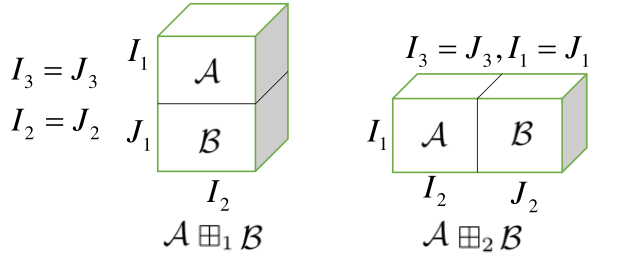
The low rank and sparse matrix decomposition has been improved by the [13]. The main idea is incorporating multi-scale structures with low rank methods. The additional multi-scale structures can obtain a more accurate representation than conventional low rank methods. Inspired by this work, we notice that the sparse component in matrix is block-distributed in some applications, e.g. shadow and motion in videos. For these images we find it is more effective to extract the low rank components in a another smaller scale of image data. Here we try to extract low rank components in block tensor data that is stacked by small scale of image data. And when we decompose the tensor data into many small blocks, it is easy to extract the principal component in some blocks that have few sparse components. We model our tensor data as the concatenation of block tensors instead of solving the RPCA problem as a whole big tensor. Fig. 2 is the illustration of concatenation of block tensors.

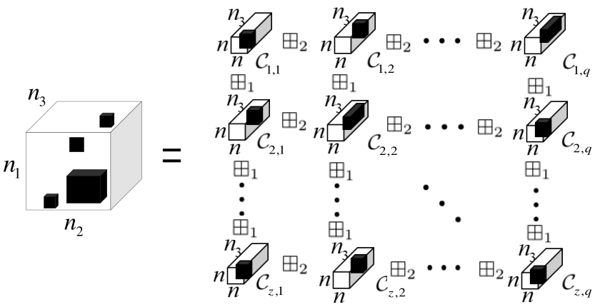
Based on the above motivation, we decompose the whole tensor into concatenation of blocks of the same size, then we extract low rank component of each block by minimizing the tubal rank of each block tensor. Fig. 3 is the illustration of our method. And we get low rank component of the whole tensor by concatenating all the low rank components of the block tensors. The proposed method can be used to some conventional image processing problems, including motion separation for surveillance videos (Section 4.1) and illumination normalization for face images (Section 4.2). The results of numerical experiments demonstrate that our method outperforms the existing methods in term of accuracy.

In this section, we describe the notations and definitions used throughout the paper briefly [14, 15, 16, 17].

A third-order tensor is represented as $\mathcal{A}$, and its (i, j, k)-th entry is represented as $\mathcal{A}_{i,j,k}$. $\mathcal{A}(i,j,:)$ denotes the (i, j)-th tubal scalar. $\mathcal{A}(i,:,:)$, $\mathcal{A}(:,j,:)$ and $\mathcal{A}(:,:,k)$ are the i-th horizontal, j-th lateral and k-th frontal slices, respectively.$\lVert\mathcal{A}\rVert_{\mathrm{F}}=\sqrt{\sum_{i,j,k}|a_{ijk}|^{2}}$ and $\lVert\mathcal{A}\rVert_{\mathrm{\infty}}=\text{max}_{i,j,k}|a_{ijk}|$ tensor kinds of tensor norms.

We can view a three-dimensional tensor of size $\emph{n}_{1}\times\emph{n}_{2}\times\emph{n}_{3}$ as an $\emph{n}_{1}\times\emph{n}_{2}$ matrix of tubes. $\hat{\mathcal{A}}$ is a tensor which is obtained by taking the fast Fourier transform (FFT) along the third mode of $\mathcal{A}$. For a compact notation we will use $\hat{\mathcal{A}}$ = fft $(\mathcal{A},[],3)$ to denote the FFT along the third dimension. In the same way, we can also compute $\mathcal{A}$ from $\hat{\mathcal{A}}$ using the inverse FFT (IFFT).

Definition 2.1 (t-product) [12] The t-product $\mathcal{E}=\mathcal{A}*\mathcal{B}$ of $\mathcal{A}\in\mathbb{R}^{\emph{n}_{1}\times\emph{n}_{2}\times\emph{n}_{3}}$ and $\mathcal{B}\in\mathbb{R}^{\emph{n}_{2}\times\emph{n}_{4}\times\emph{n}_{3}}$ is an $\emph{n}_{1}\times\emph{n}_{4}\times\emph{n}_{3}$ tensor. The $(i,j)$-th tube of $\mathcal{E}$ is given by

where $\bullet$ denotes the circular convolution between two tubes of same size.

Definition 2.2 (conjugate transpose) [14] The conjugate transpose of a tensor $\mathcal{A}$ of size $\emph{n}_{1}\times\emph{n}_{2}\times\emph{n}_{3}$ is the $\emph{n}_{2}\times\emph{n}_{1}\times\emph{n}_{3}$ tensor $\mathcal{A}^{\mathrm{T}}$ obtained by conjugate transposing each of the frontal slice and then reversing the order of transposed frontal slices from 2 to $\emph{n}_{3}$.

Definition 2.3 (identity tensor) [14] The identity tensor $\mathcal{I}\in\mathbb{R}^{\emph{n}\times\emph{n}\times\emph{n}_{3}}$ is a tensor whose first frontal slice is the $\emph{n}\times\emph{n}$ identity matrix and all other frontal slices are zero.

Definition 2.4 (orthogonal tensor) [14] A tensor $\mathcal{Q}$ is orthogonal if it satisfies

Definition 2.5 (f-diagonal tensor) [14] A tensor is called f-diagonal if each of its frontal slices is a diagonal matrix.

Definition 2.6 (t-SVD) [14] For $\mathcal{A}\in\mathbb{R}^{\emph{n}_{1}\times\emph{n}_{2}\times\emph{n}_{3}}$ , the t-SVD of $\mathcal{A}$ is given by

where $\mathcal{U}$ and $\mathcal{V}$ are orthogonal tensors of size $\emph{n}_{1}\times\emph{n}_{1}\times\emph{n}_{3}$ and $\emph{n}_{2}\times\emph{n}_{2}\times\emph{n}_{3}$ respectively, and $\mathcal{S}$ is a f-diagonal tensor of size $\emph{n}_{1}\times\emph{n}_{2}\times\emph{n}_{3}$.

We can obtain this decomposition by computing matrix singular value decomposition (SVD) in the Fourier domain, as it shows in Algorithm 1. Fig. 4 illustrates the decomposition for the three-dimensional case.

Definition 2.7 (tensor multi-rank and tubal rank) [9] The tensor multi-rank of $\mathcal{A}\in\mathbb{R}^{\emph{n}_{1}\times\emph{n}_{2}\times\emph{n}_{3}}$ is a vector $\mathbf{r}\in\mathbb{R}^{\emph{n}_{3}}$ with its i-th entry as the rank of the i-th frontal slice of $\hat{\mathcal{A}}$, i. e. $\emph{r}_{i}=\mathrm{rank}(\hat{\mathcal{A}}(:,:,i))$. The tensor tubal rank, denoted by $\mathrm{rank_{t}}(\mathcal{A})$, is defined as the number of nonzero singular tubes of $\mathcal{S}$, where $\mathcal{S}$ is from $\mathcal{A}=\mathcal{U}*\mathcal{S}*\mathcal{V^{\mathrm{T}}}$, i. e.

Definition 2.8 (tensor nuclear norm: TNN) [9] The tensor nuclear norm of$\mathcal{A}\in\mathbb{R}^{\emph{n}_{1}\times\emph{n}_{2}\times\emph{n}_{3}}$ denoted by $\|\mathcal{A}\|_{*}$ is defined as the sum of the singular values of all the frontal slices of $\hat{\mathcal{A}}$. The TNN of $\mathcal{A}$ is equal to the TNN of blkdiag($\hat{\mathcal{A}}$). Here blkdiag($\hat{\mathcal{A}}$) is a block diagonal matrix defined as follows:

where $\hat{\mathcal{A}}^{(i)}$ is the i-th frontal slice of $\hat{\mathcal{A}},i=1,2,...,n_{3}$.

Definition 2.9 (standard tensor basis) [12] The column basis, denoted as $\mathring{\mathfrak{e}}_{i}$, is a tensor of size $\emph{n}\times{1}\times\emph{n}_{3}$ with its (i,1,1)-th entry equaling to 1 and the rest equaling to 0. Naturally its transpose $\mathring{\mathfrak{e}}_{i}^{\mathrm{T}}$ is called row basis.

We decompose the whole tensor which satisfies the incoherence conditions into many small blocks of the same size. And the third dimension of the block size should be the same as the third dimension of the tensor. That is to say, given an input tensor $\mathcal{X}\in\mathbb{R}^{\emph{n}_{1}\times\emph{n}_{2}\times\emph{n}_{3}}$ and its corresponding block size, we propose a multi-block tensor modeling that models the tensor data $\mathcal{X}$ as the concatenation of block tensors. And each block tensor can be decomposed into two components, i.e. $\mathcal{X}_{p}=\mathcal{L}_{p}+\mathcal{S}_{p},~p=1,\cdots,P$, where $\mathcal{L}_{p}$ and $\mathcal{S}_{p}$ denote the low rank component and sparse component of block tensor $\mathcal{X}_{p}$ respectively.

As observed in RPCA, the low rank and sparse decomposition is impossible in some cases [4]. Similarly, we are not able to identify the low rank component and sparse component if the tensor is of both low rank and sparsity. Similar to the tensor incoherence conditions [8], we assume the block tensor data $\mathcal{L}_{p}$ in each block satisfies some block tensor incoherence conditions to guarantee successful low rank component extraction.

Definition 3.1 (block tensor incoherence conditions) For $\mathcal{L}_{p}\in\mathbb{R}^{\emph{n}\times\emph{n}\times\emph{n}_{3}}$, assume that $\mathrm{rank_{t}}(\mathcal{L}_{p})=r$ and it has the t-SVD $\mathcal{L}_{p}=\mathcal{U}_{p}*\mathcal{S}_{p}*\mathcal{V}_{p}^{\mathrm{T}}$, where $\mathcal{U}_{p}\in\mathbb{R}^{\emph{n}\times\emph{r}\times\emph{n}_{3}}$ and $\mathcal{V}_{p}\in\mathbb{R}^{\emph{n}\times\emph{r}\times\emph{n}_{3}}$ satisfy $\mathcal{U}_{p}^{\mathrm{T}}*\mathcal{U}_{p}=\mathcal{I}$ and $\mathcal{V}_{p}^{\mathrm{T}}*\mathcal{V}_{p}=\mathcal{I}$, and $\mathcal{S}_{p}\in\mathbb{R}^{\emph{r}\times\emph{r}\times\emph{n}_{3}}$ is an f-diagonal tensor. Then $\mathcal{L}_{p}$ satisfies the tensor incoherence conditions with parameter $\mu$ if

and

The incoherence condition guarantees that for small values of $\mu$, the singular vectors are not sparse. Then the tensor $\mathcal{L}_{p}\in\mathbb{R}^{\emph{n}\times\emph{n}\times\emph{n}_{3}}$ can be decomposed into low rank component and sparse component.

For extracting the low rank component from every block, we process the tensor nuclear norm of $\mathcal{L}_{p}$, i. e. $\lVert\mathcal{L}_{p}\rVert_{\mathrm{TNN}}=\lVert\mbox{blkdiag}(\hat{\mathcal{L}_{p}})\rVert_{*}$. Here we can use singular value thresholding operator in the Fourier domain to extract the low rank component of the block tensor [18, 19]. The proposed method is called iterative block tensor singular value thresholding (IBTSVT). The thresholding operator used here is the soft one $D_{\tau}$ as follows:

where “$()_{+}$” keeps the positive part.

After we extract the low rank component $\mathcal{L}=\mathcal{L}_{1}\boxplus\mathcal{L}_{2}\boxplus\cdots\boxplus\mathcal{L}_{P}$, where $\boxplus$ denotes concatenation operation, we can get the sparse component of the tensor by computing the $\mathcal{S}=\mathcal{X}-\mathcal{L}$. See Algorithm 2 in details.

In our method, the block size can’t be too large. The large size of the block will make the sparse part contain some low rank component. And if the size of the block is too small, the computational time will be long. Because the number of t-SVDs is large. Generally, we can choose our block size $2\times 2\times n_{3}$.

In our algorithm, we choose $\mu=1.8$, $\eta=1$, $\epsilon=10^{-2}$. But the thresholding parameter $\tau$ is difficult to determine. Here we can get a value by experience. As discussed in [8], the thresholding parameter could be $\tau=1/\sqrt{nn_{3}}$ for every block. This value is for denoising problem in images or videos, where the noise is uniformly distributed. But for different applications, it should be different from $1/\sqrt{nn_{3}}$. Because in these applications, the sparse component in data is not uniformly distributed, such as shadow in face images and motion in surveillance videos.

In this section, we conduct numerical results to show the performance of the method. We apply IBTSVT method on two different real datasets that are conventionally used in low rank model: motion separation for surveillance videos (Section 4.1) and illumination normalization for face images (Section 4.2).

In this paper, we proposed a novel IBTSVT method to extract the low rank component of the tensor using t-SVD. The IBTSVT is a good way to utilize the structural feature of tensor by solving TPCA problem in block tensor form. We have given the tensor incoherence conditions for block tensor data. For applications, we considered motion separation for surveillance videos and illumination normalization for face images, and numerical experiments showed its performance gains compared with the existing methods.

This work is supported by National High Technology Research and Development Program of China (863, No. 2015AA015903), National Natural Science Foundation of China (NSFC, No. 61602091, No. 61602091), the Fundamental Research Funds for the Central Universities (No. ZYGX2015KYQD004, No. ZYGX2015KYQD004), and a grant from the Ph.D. Programs Foundation of Ministry of Education of China (No. 20130185110010).

References

- [1] T. G. Kolda and J. Sun, “Scalable tensor decompositions for multi-aspect data mining,” in IEEE International Conference on Data Mining. IEEE, 2008, pp. 363–372.
- [2] J. Friedman, T. Hastie, and R. Tibshirani, The elements of statistical learning, vol. 1, Springer series in statistics Springer, Berlin, 2001.
- [3] I. Jolliffe, Principal Component Analysis, New York: Springer, 2002.
- [4] E. J. Candès, X. Li, Y. Ma, and J. Wright, “Robust principal component analysis,” Journal of the ACM, vol. 58, no. 3, pp. 1–73, 2011.
- [5] Y. Peng, A. Ganesh, J. Wright, W. Xu, and Y. Ma, “RASL: robust alignment by sparse and low-rank decomposition for linearly correlated images,” IEEE Transactions on Pattern Analysis and Machine Intelligence, vol. 34, no. 11, pp. 2233–2246, 2010.
- [6] L. Li, W. Huang, I. Y. H. Gu, and Q. Tian, “Statistical modeling of complex backgrounds for foreground object detection,” IEEE Transactions on Image Processing, vol. 13, no. 11, pp. 1459–72, 2004.
- [7] A. S. Georghiades, P. N. Belhumeur, and D. J. Kriegman, “From few to many: Illumination cone models for face recognition under variable lighting and pose,” IEEE Transactions on Pattern Analysis and Machine Intelligence, vol. 23, no. 6, pp. 643–660, 2001.
- [8] C. Lu, Y. Chen J. Feng, W. Liu, Z. Lin, and S. Yan, “Tensor robust principal component analysis: Exact recovery of corrupted low-rank tensors via convex optimization,” in The IEEE Conference on Computer Vision and Pattern Recognition, June 2016.
- [9] Z. Zhang, G. Ely, S. Aeron, N. Hao, and M. Kilmer, “Novel methods for multilinear data completion and de-noising based on tensor-svd,” Computer Science, vol. 44, no. 9, pp. 3842–3849, 2014.
- [10] A. Cichocki, D. Mandic, L. De Lathauwer, G. Zhou, Q. Zhao, C. Caiafa, and H. A. Phan, “Tensor decompositions for signal processing applications: From two-way to multiway component analysis,” IEEE Signal Processing Magazine, vol. 32, no. 2, pp. 145–163, 2014.
- [11] L. De Lathauwer, B. De Moor, and J. Vandewalle, “A multilinear singular value decomposition,” SIAM Journal on Matrix Analysis and Applications, vol. 21, no. 4, pp. 1253–1278, 2000.
- [12] Z. Zhang and S. Aeron, “Exact tensor completion using t-svd,” arXiv preprint arXiv:1502.04689, 2015.
- [13] F. Ong and M. Lustig, “Beyond low rank + sparse: Multiscale low rank matrix decomposition,” IEEE Journal of Selected Topics in Signal Processing, vol. 10, no. 4, pp. 672–687, 2015.
- [14] M. E. Kilmer and C. D. Martin, “Factorization strategies for third-order tensors,” Linear Algebra and its Applications, vol. 435, no. 3, pp. 641–658, 2011.
- [15] K. Braman, “Third-order tensors as linear operators on a space of matrices,” Linear Algebra and Its Applications, vol. 433, no. 7, pp. 1241–1253, 2010.
- [16] M. E. Kilmer, E. Misha, K. Braman, N. Hao, and R. C. Hoover, “Third-order tensors as operators on matrices: a theoretical and computational framework with applications in imaging,” SIAM Journal on Matrix Analysis and Applications, vol. 34, no. 1, pp. 148–172, 2013.
- [17] T. G. Kolda and B. W. Bader, “Tensor decompositions and applications,” SIAM Review, vol. 66, no. 4, pp. 294–310, 2005.
- [18] J. F. Cai, E. J. Candès, and Z. Shen, “A singular value thresholding algorithm for matrix completion,” SIAM Journal on Optimization, vol. 20, no. 4, pp. 1956–1982, 2008.
- [19] G. A. Watson, “Characterization of the subdifferential of some matrix norms,” Linear Algebra and Its Applications, vol. 170, no. 6, pp. 33–45, 1992.
- [20] R. Basri and D. W. Jacobs, “Lambertian reflectance and linear subspaces,” IEEE Transactions on Pattern Analysis and Machine Intelligence, vol. 25, no. 2, pp. 218–233, 2003.
- [21] P. Viola and M. Jones, “Rapid object detection using a boosted cascade of simple features,” in Computer Vision and Pattern Recognition. IEEE, 2001, vol. 1, pp. I–511.