Optimal Elephant Flow Detection
Abstract
Monitoring the traffic volumes of elephant flows, including the total byte count per flow, is a fundamental capability for online network measurements. We present an asymptotically optimal algorithm for solving this problem in terms of both space and time complexity. This improves on previous approaches, which can only count the number of packets in constant time. We evaluate our work on real packet traces, demonstrating an up to X2.5 speedup compared to the best alternative.
| Algorithm | Space | Query Time | Update Time | Deterministic |
|---|---|---|---|---|
| Space Saving [14] | ✓ | |||
| CM Sketch [16] | ✗ | |||
| Count Sketch [11] | ✗ | |||
| This Paper- IM-SUM | amortized | ✓ | ||
| This Paper- DIM-SUM | worst case | ✓ |
I Introduction
I-A Background
Network monitoring is at the core of many important networking protocols such as load balancing [6, 21], traffic engineering [9, 43], routing, fairness [29], intrusion and anomaly detection [25, 39, 46], caching [23], policy enforcement [41] and performance diagnostics [18]. Effective network monitoring requires maintaining various levels of traffic statistics, both as an aggregate and on a per-flow basis. This includes the number of distinct flows, also known as flow cardinality, the number of packets generated by each flow, and the total traffic volume attributed to each flow. Each of these adds complementing capabilities for managing and protecting the network. For example, a large increase in cardinality may indicate a port-scanning attack, while statistics about the number of packets or the volume of traffic can help perform load balancing, meet QoS guarantees and detect denial-of-service (DoS) attacks. For the latter, identifying the top- flows, or the heavy-hitters and elephant flows are essential competencies. Similarly, traffic engineering [9] involves detecting high volume flows and ensuring that they are efficiently routed.
Operation speed is of particular importance in network measurement. For example, a reduction in latency for partition/aggregate workloads can be achieved if we are able to identify traffic bursts in near real time [18]. The main challenges in addressing the above mentioned tasks come from the high line rates and large scale of modern networks. Specifically, to keep up with ever growing line rates, update operations need to be extremely fast. As already mentioned, when near real-time decisions are expected, queries should also be answered quickly. In addition, due to the huge number of flows passing through a single network device, memory is becoming a major concern. In a hardware implementation, the data structures should fit in TCAM or SRAM, because DRAM is too slow to keep up with line rate updates. Similarly, in a software implementation, as can be envisioned in upcoming SDN and NFV realizations, the ability to perform computations in a timely manner greatly depends on whether the data structures fit in the hardware cache and whether the relevant memory pages can be pinned to avoid swapping.
While the problem of identifying the top- flows and heavy-hitters in terms of the number of packets has been addressed by many previous works, e.g., [7, 19, 30, 37], detection of elephant flows in terms of their traffic volume has received far less attention. However, it is non-trivial to translate a top- or heavy-hitters algorithm to an efficient elephant flow solution, because many of the former maintain ordered or semi-ordered data structures [7, 19, 30, 37]. Performing fast updates to these data structures depends on the fact that each packet increments (or decrements) its corresponding counter(s) by . Hence, the perturbation caused by each update is fairly contained, predictable and tractable. In contrast, when each packet modifies its corresponding counter(s) by its entire size, such maintenance becomes much harder. Further, treating an increment (or decrement) by the packet’s size as a sequence of increments (or decrements) by would multiply the update time by a factor of , rendering it too slow.
I-A1 Contributions
In this paper, we introduce the first elephant flow detection scheme that provides the following benefits: () constant time updates, () constant time point-queries, () detection of elephant flows in linear time, which is optimal, and () asymptotically optimal space complexity. This is achieved with two hash-tables whose size is proportional to the number of elephant flows, and a single floating point variable. We present two flavors of the algorithm for maintaining these data structures. The first version Iterative Median SUMming (IM-SUM), which is easier to describe and simpler to code, works in amortized time. The second variant De-amortized Iterative Median SUMming (DIM-SUM) de-amortizes the first, thereby obtaining worst case execution time.
We also evaluate the performance of these variants on both synthetic and real-world traces, and compare their execution time to other leading alternatives. We demonstrate that IM-SUM is up to 2.5 times faster than any of our competitors on these traces, and up to an order of magnitude faster than others. DIM-SUM is slower than IM-SUM, but still faster than all competitors for small values of . DIM-SUM is faster in terms of worst case guarantee, ensuring constant update time. The latter is important when real-time behavior is required.
I-B Related work
Network monitoring capabilities are needed in both hardware and software [38]. In hardware, space is a critical constraint as there is no sufficient memory technology; while SRAM is fast enough to operate at line speed, it is too small to accommodate all flows. On the contrary, DRAM is too slow to be read at line speed. Traditional network monitoring approaches utilized short probabilistic counters [22, 42, 44] to reduce the memory requirements.
Counter arrays are managed by network devices [22, 42, 44] as well as sketches such as the Count Sketch [11] and the Count Min Sketch (CM-Sketch) [16]. These algorithms can be extended to support finding frequent items using hierarchy and group testing [14, 16, 17]. As network line rates became faster, sketches evolved into more complex algorithms that require significantly less memory at the expense of a long decoding time. Such algorithms include Counter Braids [34], Randomized Counter Sharing [32] and Counter Tree [12]. While these algorithms handle updates very fast, they incur a long query time. Thus, queries can only be done off-line and not in real time as required by some networking applications.
For software implementations, counter based algorithms are often the way to go [14]. These methods typically maintain a flow table, where each monitored flow receives a table entry. Counter algorithms differ from one another in the the flow table maintenance. Specifically, in Lossy Counting [36], new flows are always added to the table. In order to keep the table size bounded, flow counters are periodically decremented and flows whose counters reach 0 are deleted. Lossy counting is simple and effective, but its space consumption is not optimal. Lossy Counting’s space consumption was empirically improved with probabilistic eviction of entries [20] as well as statistical knowledge about the stream distribution [40] that allows dropping excess table entries earlier.
Frequent (FR) [30] is a space optimal algorithm [31]. In FR, instead of decrementing counters periodically, when a packet arrives for a non resident flow and the table is full, all counters are decremented. This improves the space complexity to optimal, but flow counters are needlessly decremented and therefore the algorithm is less accurate. This is solved by the Space Saving algorithm [37]. In Space Saving, when a packet that belongs to a flow that does not have a counter arrives, and the flow table is full, the algorithm evicts the entry whose counter is minimal. The rest of the counters are untouched and their estimation is therefore more accurate. For packet counting, since all counter updates are , Space Saving and FR can be implemented in [7, 37]. This makes Space Saving and FR asymptotically optimal in both space and time. The version of Space Saving we compare against in this paper uses a heap to manage its counters [14, 15, 35]; we denote it hereafter SSH. In the general case, packets have different sizes so SSH requires a logarithmic runtime. This is preferred over the original implementation with ordered linked lists [37], which requires a constant time to count the number of packets but a linear time when considering packet sizes.
Various methods such as a sketches for tail items and a randomized counter admission policy can make (empirically) more efficient data structures [27, 8]. These improvements are orthogonal to the one presented in this paper.
Alternatively, [5] implemented elephant flow identification with a Sample and Hold like technique [36]. That is, the controller receives sampled packets and periodically updates the monitored flows to reflect the current state of the heavy hitters. Unfortunately, sampling discards some of the information about packet sizes that can be used to reduce the error. In addition, since sampling does not take into account the packet size, large packets can be missed, resulting in a large error.
In general, space is required to approximately count with an additive error bounded by , where is the total weight of all items in the stream [37]. The optimal runtime is for both update and query. Related works which are capable of estimating flow volume (rather than packet counting) are summarized in Table I. As listed, our algorithms are the first to offer both (asymptotically) optimal space consumption and optimal runtime.
II Model
We consider a stream () of tuples of the form, , where denotes item’s id and its (non-negative) weight. At each step, a new tuple is added to the stream and we denote by the current number of tuples in the stream.
Given an identifier , we denote the total weight of as:
When , we denote: .
Also, the total weight of all ids in the stream at time is:
II-A Problem definitions:
We now formally define the problems we address.
- •
- Volume Estimation: We say that an algorithm solves the - Volume Estimation problem if at any time , returns an estimation that satisfies
- •
-Elephant Flows: We say that an algorithm solves the - Elephant Flows problem if at any time , an query returns a set of elements , such that for every flow , , and . We note that if the stream is unweighted (all weights are ), this degenerates to the Heavy Hitters problem discussed in [14, 37, 45].
II-B Notations
The notations used in this paper are summarized in Table II.
| Symbol | Meaning |
|---|---|
| The total sum of all items in the stream so far. | |
| The total sum of all items in the stream until time . | |
| The weighted frequency for item in the stream so far. | |
| The weighted frequency for item , at time . | |
| An estimate of the weighted frequency of item , at time . | |
| A speed-space tradeoff parameter, affects frequency of maintenance operations and memory consumption. | |
| Accuracy parameter, small means lower estimation error but more counters. | |
| The estimate of the top quantile at time . | |
| Threshold for elephant flows. | |
| The error probability allowed in randomized algorithms. |
III Solution
III-A Intuition
Ideally, when the table is full, we wish to evict the smallest flow as in Space Saving. However, in the weighted case, Space Saving runs in logarithmic time. We achieve constant runtime by relaxing the memory constraint; instead of removing the minimal flow upon arrival of a non resident flow, we periodically remove many small flows from the table at once. This maintenance operation takes linear time, but it is invoked infrequently enough to achieve amortized runtime. The table size only increases by a constant factor, so our solution remains (asymptotically) space optimal.
In principle, an optimal algorithm requires space [10], and runs in constant time. The algorithm provides an approximation guarantee that the error is bounded by where is the total weight of all flows in the stream.
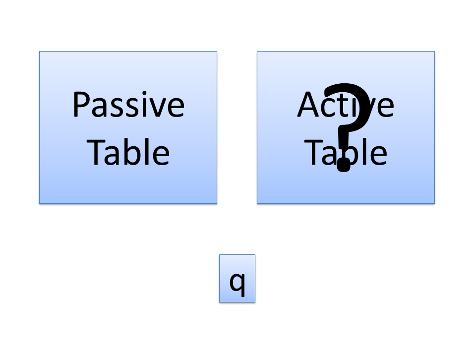
Intuitively, our periodic maintenance process identifies the largest counter, and evicts all flows whose counters is smaller than that counter. This is obtained by internally splitting the table into two sub-tables named Active and Passive. Each table entry contains both the flow’s id and a counter that represents the flow’s volume. The Active table is mutable, while the Passive is read-only. That is, updates only affect the Active table while queries consider both of them. The maintenance process copies all counters that are larger than the quantile of the largest flow from the Passive table to the Active table, clears the Passive table, and then switches between them. That way, the size of the Active and Passive tables remains bounded while the largest flows are never evicted.
Each table is configured to store at most: items, where is a positive constant that affects a speed-space trade off as explained below. In addition, we keep a single floating point variable , which represents the value of the last quantile calculated. is the default estimation returned when querying the frequency of non-resident flows. It ensures that such estimates meet the maximum error guarantee.
We then improve the complexity to worst case with a de-amortization process. Intuitively, this is done by performing a small piece of the maintenance prior to each update. We need to make sure that maintenance is always finished by the time the Active table fills up. Once maintenance is over, we switch the Active table with the (now empty) Passive table.

III-B Iterative Median Summing
We describe our Iterative Median SUMming (IM-SUM) algorithm and its deamortized variant Deamortized Iterative Median SUMming (DIM-SUM), by detailing four operations: a query operation, which computes the volume of a flow; an elephants method that returns all elephant flows; an update operation, which increases the volume of a flow corresponding to a recently arrived packet; and a maintenance operation, which periodically discards infrequent flows to prevent overflowing.
The query procedure appears in Figure 1. As depicted, the estimated weighted frequency of element , , is if has an Active table entry, if has a Passive table entry and otherwise .
Returns the elephant flows. First, we set ; then, we traverse both the Active and Passive tables, adding to any flow for which .

Update
The update procedure is illustrated in Figure 2. The procedure deals with an arrival of a pair (flow id, weight), e.g., may be a TCP five tuple and the byte size of its payload. In the update procedure, we first perform a query for . Let be the query result for . We add the following entry to the Active table: .


Maintenance
As mentioned above, we require periodic maintenance to keep the Active table from overflowing. We define generation in the stream; a generation starts/ends every time the Active table fills up. Before a generation ends, the maintenance process needs to achieve the following:
- 1.
Set to be the largest value in the Passive table.
- 2.
Move or copy all items with frequency larger than from the Passive table to the Active table, except for the items that already appear in the Active table.
- 3.
Clear the Passive table.
- 4.
When the Active Table has filled, switch the Active and Passive tables before a new generation begins. After the switch, the Active table is empty and the Passive contains all entries that were a part of the Active table.
The maintenance process is illustrated in Figure 3. Maintenance operations are performed once per generation and we need to guarantee that the number of items in the Active table never exceeds the allocated size of . We later prove that the number of update operations between two consecutive maintenance operations is at least , and show that as a result the update time is constant if is constant.
III-C Maintenance Implementation
There are several ways to implement the maintenance steps described in Section III-B, which provide different runtime guarantees. Section III-C1 explains that when the maintenance operation is run serially after the Active table fills up we achieve an amortized runtime, while Subsection III-C2 explains how to improve the runtime to worst case.
III-C1 Simple Maintenance
In this suggestion, we perform the maintenance procedure serially at the end of each generation. The most computationally intensive step is Step 1, where we need to find the largest counter. When , this value is the median, and as long as is constant, it is a certain percentile. It is well known that median (and other percentiles) can be calculated in linear time in a deterministic manner, e.g., by using the median of medians algorithm. Therefore, the time complexity of Step 1 is linear with the table size of .
In Step 2, we copy at most entries from the Passive table to the Active table. The complexity of this step is . Step 3 can be performed in time or in time, depending if the hash table supports constant time flush operations. Finally, Step 4 requires time. Therefore, since the number of update operations in a generation is , as shown in Lemma 2, the average update time per packet is , which is when is constant. Therefore, the simple maintenance procedure can be executed with amortized time. As mentioned above, we nickname our algorithm with the simple maintenance procedure Iterative Median SUMming (IM-SUM).
III-C2 De-amortized Implementation
In deamortization, we can perform only a small portion of the maintenance procedure on each packet arrival. The challenge is to evenly split the maintenance task between update operations. Our deamortized algorithm, nicknamed De-amortized Iterative Median SUMming (DIM-SUM), uses the following two techniques.
Controlled Execution
Here, we execute maintenance operations after processing each packet. Since the total maintenance time is , we divide the maintenance to tasks of operations each and execute a single task for each update operation. Therefore, when is chosen to be a constant, we achieve worst case complexity.
Note that we do not know how many update operations will actually occur before the Active table fills, e.g., if a flow with an Active table entry is updated, then the number of Active table entries does not increase. This motivates us to dynamically adjust the size of the maintenance operations according to the workload, to avoid a large variance in the length of update operations. If we use the static bound proven above, the first update operations will be slow, and once maintenance is over, update operations will be fast. To avoid this situation, we suggest an approach to dynamically adjust the task size according to the actual workload.
To do so, prior to each update operation, we recalculate the minimum number of remaining updates according to the actual number of entries in the Active table and the maximal number of entries that still need to be copied from the Passive table. Next, we calculate the maximum number of operations left in the current maintenance iteration. Before each update operation, we execute maintenance operations.
Double Threading
A second approach is to run some of the maintenance steps in a second thread in parallel to the update operations. We should ascertain that a sufficient number of maintenance operations are executed with every update operation. This resembles a producer-consumer problem, where the maintenance thread is the producer and the update thread is the consumer. It can be implemented with a semaphore. After a sufficient number of maintenance operations is executed, the semaphore increments, and before an update operation is executed, the semaphore decrements.
While the above technique requires synchronization between the two threads, it has a few advantages. First, it simplifies the implementation. The calculation of a quantile is usually performed with a recursive function. Therefore, freezing the calculation and resuming it later requires saving the trace of recursive calls. Second, the double-threading procedure enables running the update and the maintenance procedures in parallel, which can save time. The drawback of this technique is the use of semaphore for synchronization, which hurts performance.
III-D What is in a Hash Table?
The only data structure used by our solution is a hash table. This means that the hash table’s properties directly impact the performance of our solution. In particular, advances in hash tables (e.g., [24]) can directly improve our work.
Below, we survey some interesting possibilities.
III-D1 Do we really need two different tables?
In principle, one could implement both Active and Passive tables as a single table with a bit that decides if the entry belongs to the Passive or Active table. This approach can speed up the maintenance process, as moving an item from the Passive to the Active table can be done by flipping a bit, which can even be done in an atomic manner.
III-D2 Cuckoo Hash Table
Cuckoo hashing is very attractive for read intensive workloads as it offers worst case queries. The trade off is that insertions end in time only with high probability.
Another interesting benefit of the Cuckoo hash table is fast delete operations; all entries below a certain threshold can be instantly removed by treating them as empty [33]. A similar technique could also be used in our case and further reduce the time required to clear the Passive table.
III-D3 Compact Hash Tables
III-D4 Fast Hash Tables
Perhaps the most obvious benefit of relying only on standard hash tables is speed. Since we do not maintain any proprietary data structures, we can potentially improve our runtime as faster hash tables are developed. For example, Hop Scotch Hashing [26] is considered one of the fastest parallel hash tables in practice.
IV Analysis
IV-A Correctness
Our goal is to prove that IM-SUM and DIM-SUM solve the - Volume Estimation and - Elephant Flows problems. To do so, we first bound the value of .
Lemma 1.
at all times .
Proof of Lemma 1.
Let be the sum of the items in the tables with the largest estimation value at time . We show by induction on that for any time . Assume that .
When an item arrives at time , if it is already one of the largest items, then both and increase by , and consequently .
If was not one of the largest items at time and has not become one at time , then .
If, however, was not one of the largest items at time but became one at time , mark the frequency of the largest item by . If there are fewer than items in the tables, define . After adding , the estimation of () becomes at most . Therefore adds to up to . Fortunately, if , then there must be at least items with a positive estimation, and since has become one of the largest items, it must have replaced an item with frequency at least . Therefore, we subtract at least from . In case was , we still subtract from . Either way,
Thus for every .
We next consider the time at the beginning of a generation before was computed. There cannot be items larger than , or otherwise would be larger than . Since this is the beginning of the generation, all of the items are in the passive table, and the quantile will be computed on the current items. Therefore will be smaller or equal to . Since the sum of elements only grows, . ∎
Theorem 1.
Our algorithm solves - Volume Estimation: That is, at any step (): .
Proof.
We prove the theorem by induction over the number of elements seen .
Basis: At time , the claim holds trivially.
Hypothesis: Suppose that at time some element has an approximation
Step: Assume that at time item arrives with weight . If , then the new estimation grows by exactly , same as the true weight of . According to the induction hypothesis, the estimation remains correct. Similarly, when another item arrives at time , does not change, and neither does . Steps 1 , 2 and 4 do not change the estimation for any item.
During step 3, however, could be removed from the Passive table. If is also in the Active table, remains the same. Otherwise, is changed from to . However, since only appears in the Passive table, we deduce that it was not moved in step 2. This means that the estimation for at the beginning of the generation was smaller or equal to . Therefore, it is immediate from the induction hypothesis that . After is removed from the Passive table as well, the estimation becomes . Hence, .
Lemma 1 proves that and therefore we have .
∎
Next, we prove that our algorithm is also able to identify the elephant flows. We note that the runtime is optimal as there could be elephant flows.
Theorem 2.
At any time , the query solves - Elephant Flows in time.
Proof.
Queries are done by traversing the tables and observing all elements such that . The tables are of size when is constant and therefore the complexity is .
Let be such that . According to Theorem 1 and Lemma 1, . Hence, must appear in one of the tables with frequency greater than . Otherwise, it would have an estimation of less than . Consequently, .
Next, let be such that . According to Theorem 1, . Therefore, will not be included in . ∎
IV-B Runtime
We now prove that IM-SUM runs at amortized time and that DIM-SUM runs at worst case time. Our goal is to evaluate both the complexity of the maintenance and the number of update operations between two consecutive maintenance operations. We start with evaluating the minimal number of update operations between two consecutive generations, i.e., the number of unique flows that must be encountered before we switch to a new generation.
Lemma 2.
Denote by the minimal number of update operations between subsequent generations: .
Proof.
In the beginning of every generation the Active table is empty. During step 2, the Active table receives up to items from the Passive table. Other than that, the Active table only grows due to update operations. Therefore, there must be at least
updates in each generation. ∎
Next, we bound the number of hash table operations required to perform the maintenance process.
Lemma 3.
The maintenance process requires: hash table operations.
Proof.
We calculate the complexity of all steps. For Step 1, it is well known that a median can be found in linear time, e.g., using the median of medians algorithm. The same is true for any percentile, and therefore Step 1 requires
hash table operations to complete.
Step 2 goes over the Passive table, which is of size , and copies or moves some of the items to the Active table. Therefore, its complexity is .
Theorem 3.
For any fixed , IM-SUM runs in amortized and DIM-SUM in worst case hash table operations.
Proof.
First, we observe that for any constant , Lemma 2 establishes that there are update operations between generations. Similarly, by Lemma 3, there are hash function operations to do during each maintenance process.
In IM-SUM, maintenance is performed once per generation and thus the amortized complexity is .
In DIM-SUM, as the work is split between update operations, each update has to perform hash table operations. Let be the minimum number of update operations left in the generation at time and let be the maximum number of maintenance operations left. We show by induction that . At a in the beginning of the generation, and . Therefore, .
Assume, by induction, that for any time , . After a single update, , because otherwise the minimum number of updates at time would be smaller than . decreases to at most . Therefore, the number of maintenance operations executed at time is
The query process requires 2 hash table operations and is therefore also . ∎
IV-C Required Space
We now show that for each constant , IM-SUM and DIM-SUM require the (asymptotically) optimal table entries.
Theorem 4.
For each constant , the space complexity of IM-SUM and DIM-SUM is .
Proof.
The proof follows from the selected table sizes. Each table is sized to contain a maximum of entries and therefore the total number of table entries is . ∎
V Evaluation


We now present an extensive evaluation for comparing our proposed algorithm with the leading alternatives. We only considered alternative algorithms that are able to count packets of variable sizes and are able to answer queries on-line.
V-A Datasets
Our evaluation includes the following datasets:
- 1.
The CAIDA Chicago Anonymized Internet Trace 2015 [2] , denoted Chicago. The trace was collected by the ‘equinix-chicago’ high-speed monitor and contains a mix of 6.3M TCP, UDP and ICMP packets. The weight of each packed is defined as the size of its payload, not including the header.
- 2.
The CAIDA San Jose Anonymized Internet Trace 2014 [3] , denoted SanJose. The trace was collected by the ‘equinix-sanjose’ high-speed monitor and contains a mix of 20.2M TCP, UDP and ICMP packets. The weight of each packet is defined as the size of its payload, not including the header.
- 3.
The UCLA Computer Science department TCP packet trace (denoted UCLA-TCP) [4]. This trace contains 16.5M TCP packets passed through the border router of the Computer Science Department, University of California, Los Angeles. The weight of each packet is defined as the size of its payload, not including the header.
- 4.
UCLA-UDP [4]. This trace contains 18.5M UDP packets passed through the border router of the Computer Science Department, UCLA. The weight of each packet is defined as the size of its payload, not including the header.
- 5.
YouTube Trace (referred to as YouTube) [47]. The trace contains a sequence of 436K accesses to YouTube’s videos made from within the University of Massachusetts Amherst. The weight of each video is defined as its length (in seconds). An example application for such measurement is the caching of videos according to their bandwidth usage to reduce traffic.
- 6.
(Unweighted) Zipf streams that contain a series of i.i.d elements sampled according to a Zipfian distribution of a given skew. We denote a Zipf stream with skew as Zipf. Each packet is of weight .


V-B Implementation
We compare both IM-SUM and DIM-SUM [1] to Count Min Sketch (CM), a Hierarchical CM-sketch (CMH), which is an extended version of CM suited to find frequent items [13], a robust implementation of the Count Sketch that has been extended using Adaptive Group Testing by [14] to support finding Frequent Items (AGT), and a heap based implementation of Space Saving (denoted SSH) [15, 35]. The code for the competing algorithms is the one released by [14]. All implementations are in C++ and the measurements were made on a 64-bit laptop with a 2.30GHz CPU, 4.00 GB RAM, 2 cores and 4 logical cores. In our own algorithms, we used the same hash table that was used to implement SSH for fairness.
V-C The effect of
Recall that is a performance parameter; increasing increases our space requirement but also makes maintenance operations infrequent and therefore potentially improves performance. Figure 4 shows the performance of IM-SUM and DIM-SUM for values of ranging from to and . The YouTube trace seems to benefit from larger until , Chicago until , and UCLA seems to saturate around . SanJose peaks for IM-SUM at and for DIM-SUM. Zipf1.3 increases with until . The Zipf0.7 and Zipf1 traces, however, slightly decrease with . We explain the decline by an increase in memory consumption, which slows down memory access. The decline is probably not evident in other traces, because in high skew traces the effect of reducing the frequency of the maintenance procedure is larger than the effect of decreasing the memory requirement. In order to balance speed and space efficiency, we continue our evaluation with . We also recommend this setting for traces with unknown characteristics. If additional memory is available, reducing is more effective than increasing .
It is also evident that our de-amortization process has significant overheads. We attribute this to the synchronization overhead between the two threads of DIM-SUM.
V-D Effect of
Since memory consumption is coupled to accuracy , it is interesting to evaluate the operation speed as a function of . As IM-SUM and DIM-SUM are asymptotically faster, we expect them to perform better than known approaches for small s (that imply a large number of counters). Figure 5 depicts the operation speed of the algorithms, as a function of . As shown, IM-SUM is considerably faster than all alternatives in all tested workloads, even for large values of . The results for DIM-SUM are mixed. For large values, it is mostly slower than the alternatives. However, for small s, it is consistently better than previous works.
V-E Effect of Skew on operation speed
Intuitively, the higher the skew of the workload, the less frequent maintenance operations occur, because it takes longer before we see enough unique flows for the Active table to fill up. Figure 6 demonstrates the effect of the zipf skew parameter on performance. As can be observed, while CMH and AGT are quite indifferent to skew, IM-SUM and DIM-SUM benefit greatly from it and IM-SUM is faster than all alternatives. DIM-SUM is consistently faster than CMH and AGT, and has similar speed to SSH. CM is slightly faster than DIM-SUM for low skew workloads but more than three times slower than DIM-SUM when the skew is high.
VI Discussion
In this paper, we have shown two variants of the first (asymptotically) space optimal algorithm that can estimate the total traffic volume of every flow as well as identify the elephant flows (in terms of their total byte count). The first variant, IM-SUM, is faster on the average case but only ensures amortized execution time, while the second variant, DIM-SUM, offers worst case time guarantee. We have benchmarked our algorithms on both synthetic and real-world traces and have demonstrated their superior performance.
Looking into the future, we hope to further reduce the actual running time of DIM-SUM to match the rate of IM-SUM. This would probably require redesigning our code to eliminate synchronization, possibly by using an existing concurrent hash table implementation. A C++ based open source implementation of this work and all other code used in this paper is available at [1].
References
- [1] IM-SUM and DIM-SUM - Open source implementation. https://github.com/kassnery/dimsum.
- [2] The CAIDA UCSD Anon. Chichago Internet Traces 2015, Dec. 17th.
- [3] The CAIDA UCSD Anon. San Jose Internet Traces 2014, June 19th.
- [4] Unpublished, see http://www.lasr.cs.ucla.edu/ddos/traces/.
- [5] Yehuda Afek, Anat Bremler-Barr, Shir Landau Feibish, and Liron Schiff. Sampling and large flow detection in sdn. In ACM SIGCOMM, pages 345–346, 2015.
- [6] Mohammad Al-Fares, Sivasankar Radhakrishnan, Barath Raghavan, Nelson Huang, and Amin Vahdat. Hedera: Dynamic flow scheduling for data center networks. In USENIX NSDI, 2010.
- [7] Ran Ben-Basat, Gil Einziger, Roy Friedman, and Yaron Kassner. Heavy hitters in streams and sliding windows. In IEEE INFOCOM, 2016.
- [8] Ran Ben-Basat, Gil Einziger, Roy Friedman, and Yaron Kassner. Randomized admission policy for efficient top-k and frequency estimation. CoRR, abs/1612.02962, 2016.
- [9] Theophilus Benson, Ashok Anand, Aditya Akella, and Ming Zhang. Microte: Fine grained traffic engineering for data centers. In ACM CoNEXT, pages 8:1–8:12, 2011.
- [10] Radu Berinde, Graham Cormode, Piotr Indyk, and Martin Strauss. Space-optimal heavy hitters with strong error bounds. In ACM PODS, 2009.
- [11] Moses Charikar, Kevin Chen, and Martin Farach-Colton. Finding frequent items in data streams. Theor. Comput. Sci., 312(1):3–15, January 2004.
- [12] Min Chen and Shigang Chen. Counter tree: A scalable counter architecture for per-flow traffic measurement. In IEEE ICNP, pages 111–122, 2015.
- [13] Pascal Cheung-Mon-Chan and Fabrice Clérot. Finding hierarchical heavy hitters with the count min sketch. In Proceedings of 4th International Workshop on Internet Performance, Simulation, Monitoring and Measurement, IPS-MOME, 2006.
- [14] Graham Cormode and Marios Hadjieleftheriou. Finding frequent items in data streams. VLDB 2008., 1(2):1530–1541, August 2008. Code: http://hadjieleftheriou.com/frequent-items.
- [15] Graham Cormode and Marios Hadjieleftheriou. Methods for finding frequent items in data streams. J. of VLDB, 19(1):3–20, 2010.
- [16] Graham Cormode and S. Muthukrishnan. An improved data stream summary: The count-min sketch and its applications. J. Algorithms, 55(1):58–75, April 2005.
- [17] Graham Cormode and S Muthukrishnan. What’s new: finding significant differences in network data streams. IEEE/ACM Transactions on Networking (TON), 13(6):1219–1232, 2005.
- [18] Andrew R. Curtis, Jeffrey C. Mogul, Jean Tourrilhes, Praveen Yalagandula, Puneet Sharma, and Sujata Banerjee. Devoflow: Scaling flow management for high-performance networks. In ACM SIGCOMM, pages 254–265, 2011.
- [19] Erik D. Demaine, Alejandro López-Ortiz, and J. Ian Munro. Frequency estimation of internet packet streams with limited space. In Proc. of the 10th Annual European Symposium on Algorithms, ESA, 2002.
- [20] Xenofontas Dimitropoulos, Paul Hurley, and Andreas Kind. Probabilistic lossy counting: An efficient algorithm for finding heavy hitters. ACM SIGCOMM Comput. Commun. Rev., 38, 2008.
- [21] Gero Dittmann and Andreas Herkersdorf. Network processor load balancing for high-speed links. In Proc. of the Int. Symp. on Performance Evaluation of Computer and Telecommunication Systems, volume 735, 2002.
- [22] G. Einziger, B. Fellman, and Y. Kassner. Independent counter estimation buckets. In IEEE INFOCOM, pages 2560–2568, 2015.
- [23] G. Einziger and R. Friedman. TinyLFU: A highly efficient cache admission policy. In Euromicro PDP, pages 146–153, 2014.
- [24] Gil Einziger and Roy Friedman. Counting with tinytable: Every bit counts! In ACM ICDCN 2016, pages 27:1–27:10.
- [25] Pedro Garcia-Teodoro, Jesús E. Díaz-Verdejo, Gabriel Maciá-Fernández, and E. Vázquez. Anomaly-based network intrusion detection: Techniques, systems and challenges. Computers and Security, pages 18–28, 2009.
- [26] Maurice Herlihy, Nir Shavit, and Moran Tzafrir. Hopscotch hashing. In 22nd Intl. Symp. on Distributed Computing, 2008.
- [27] Nuno Homem and Joao Paulo Carvalho. Finding top-k elements in data streams. Inf. Sci., 180(24):4958–4974, December 2010.
- [28] Nan Hua, Haiquan (Chuck) Zhao, Bill Lin, and Jun Xu. Rank-indexed hashing: A compact construction of bloom filters and variants. In IEEE ICNP 2008.
- [29] Abdul Kabbani, Mohammad Alizadeh, Masato Yasuda, Rong Pan, and Balaji Prabhakar. Af-qcn: Approximate fairness with quantized congestion notification for multi-tenanted data centers. In Proc. of the 18th Symposium on High Performance Interconnects, IEEE HOTI, 2010.
- [30] Richard M. Karp, Scott Shenker, and Christos H. Papadimitriou. A simple algorithm for finding frequent elements in streams and bags. ACM Trans. Database Syst., 28(1), March 2003.
- [31] E. Kranakis, P. Morin, and Y. Tang. Bounds for frequency estimation of packet streams. In SIROCCO, pages 33–42, 2013.
- [32] T. Li, S. Chen, and Y. Ling. Per-flow traffic measurement through randomized counter sharing. IEEE/ACM Transactions on Networking, 20(5):1622–1634, Oct 2012.
- [33] Yang Liu, Wenji Chen, and Yong Guan. Near-optimal approximate membership query over time-decaying windows. In IEEE INFOCOM, pages 1447–1455, 2013.
- [34] Yi Lu, Andrea Montanari, Balaji Prabhakar, Sarang Dharmapurikar, and Abdul Kabbani. Counter braids: a novel counter architecture for per-flow measurement. In Proc. of the ACM SIGMETRICS, 2008.
- [35] Nishad Manerikar and Themis Palpanas. Frequent items in streaming data: An experimental evaluation of the state-of-the-art. Data Knowl. Eng., pages 415–430, 2009.
- [36] Gurmeet Singh Manku and Rajeev Motwani. Approximate frequency counts over data streams. In Proc. of VLDB, 2002.
- [37] Ahmed Metwally, Divyakant Agrawal, and Amr El Abbadi. Efficient computation of frequent and top-k elements in data streams. In ICDT, 2005.
- [38] Masoud Moshref, Minlan Yu, and Ramesh Govindan. Resource/accuracy tradeoffs in software-defined measurement. In Proc. of the 2nd ACM SIGCOMM Workshop on Hot Topics in Software Defined Networking, HotSDN, pages 73–78, 2013.
- [39] B. Mukherjee, L.T. Heberlein, and K.N. Levitt. Network intrusion detection. Network, IEEE, 8(3), May 1994.
- [40] Qiong Rong, Guangxing Zhang, Gaogang Xie, and K. Salamatian. Mnemonic lossy counting: An efficient and accurate heavy-hitters identification algorithm. In IEEE IPCCC, pages 255–262, 2010.
- [41] Joel Sommers, Paul Barford, Nick Duffield, and Amos Ron. Accurate and efficient sla compliance monitoring. In Proc. of the Conf. on Applications, Technologies, Architectures, and Protocols for Computer Communications, SIGCOMM. ACM, 2007.
- [42] Erez Tsidon, Iddo Hanniel, and Isaac Keslassy. Estimators also need shared values to grow together. In INFOCOM, pages 1889–1897, 2012.
- [43] Vijay Vasudevan, Amar Phanishayee, Hiral Shah, Elie Krevat, David G. Andersen, Gregory R. Ganger, Garth A. Gibson, and Brian Mueller. Safe and effective fine-grained tcp retransmissions for datacenter communication. ACM SIGCOMM, pages 303–314, 2009.
- [44] Li Yang, Wu Hao, Pan Tian, Dai Huichen, Lu Jianyuan, and Liu Bin. Case: Cache-assisted stretchable estimator for high speed per-flow measurement. In IEEE INFOCOM, 2016.
- [45] Yin Zhang, Sumeet Singh, Subhabrata Sen, Nick Duffield, and Carsten Lund. Online identification of hierarchical heavy hitters: Algorithms, evaluation, and applications. ACM IMC, 2004.
- [46] Ying Zhang. An adaptive flow counting method for anomaly detection in sdn. In ACM CoNEXT, pages 25–30, 2013.
- [47] Michael Zink, Kyoungwon Suh, Yu Gu, and Jim Kurose. Watch global, cache local: Youtube network traffic at a campus network: measurements and implications. In Electronic Imaging 2008, pages 681805–681805, 2008.