跳到论文正文
W Papers独立论文阅读器 arXiv:1701.03960 论文正文 计算阅读时间 · 0%
引用这篇论文根据当前论文元数据生成,正式投稿前建议核对。


License: arXiv.org perpetual non-exclusive license
arXiv:1701.03960v2 [q-fin.MF] 22 Mar 2019

Optimal trading with a trailing stop

Tim Leung ††thanks: Department of Applied Mathematics, University of Washington, Seattle WA 98195. E-mail: timleung@uw.edu. Corresponding author.    Hongzhong Zhang ††thanks: IEOR Department, Columbia University. New York, NY 10027. E-mail: hz2244@columbia.edu.
Abstract

Trailing stop is a popular stop-loss trading strategy by which the investor will sell the asset once its price experiences a pre-specified percentage drawdown. In this paper, we study the problem of timing to buy and then sell an asset subject to a trailing stop. Under a general linear diffusion framework, we study an optimal double stopping problem with a random path-dependent maturity. Specifically, we first analytically solve the optimal liquidation problem with a trailing stop, and in turn derive the optimal timing to buy the asset. Our method of solution reduces the problem of determining the optimal trading regions to solving the associated differential equations. For illustration, we implement an example and conduct a sensitivity analysis under the exponential Ornstein-Uhlenbeck model.

Keywords:  trailing stop, stop loss, optimal stopping, drawdown, stochastic floor

JEL Classification:  C41, C61, G11

Mathematics Subject Classification (2010):  60G40, 62L15, 91G20, 91G80

1 Introduction

Trailing stops are a popular trade order widely used by proprietary traders and retail investors to provide downside protection for an existing position. In contrast to a stop-loss exit that closes a position at a fixed price, a trailing stop is characterized by a stochastic floor that moves based on the running maximum of the asset price. This provides a dynamic downside protection as the stochastic floor is automatically adjusted upward whenever the asset price moves to a new high. A trailing stop is triggered when the prevailing price of an asset falls below the stochastic floor. In essence, it allows an investor to specify a limit on the maximum possible loss while not limiting the maximum possible gain. This is particularly relevant in common trend-following strategies, and trailing stop provides an automatic trigger to exit when prices start to trend downward due to, for example, regime switching (Dai et al., 2010).

In addition to setting a trailing stop order, the investor can also use a limit order to sell at a certain price target. If the price is sufficiently high, the investor may prefer to take profit immediately, rather than waiting further with the possibility of setting off the trailing stop. The investor’s position will be liquidated by either order, whichever comes first.

In this paper, we investigate the mathematical problem of optimal timing to liquidate a position subject to a trailing stop. Mathematically, we recognize the trailing stop as a stochastic timing constraint in the sense that it installs a path-dependent random maturity into the liquidation problem, rending the problem significantly more difficult to analyze or solve. Furthermore, the investor can decide when to establish the position in the first place. This leads us to also analyze the optimal timing to enter the market. In sum, we study an optimal double stopping problem subject to a trailing stop. Using excursion theory of linear diffusion, we derive the value functions using the smallest concave majorant characterization, and discuss the effect of trailing stopping on the optimal trading strategies analytically and numerically. Among our results, we reduce the problem of finding the optimal timing strategies to solving an ODE problem, which forms the basis of our numerical scheme in determining the optimal asset acquisition and liquidation regions.

In general, a trailing stop can be defined as the first time when the asset price XX drops below f⁡(X¯)f(\overline{X}), where X¯\overline{X} is the running maximum process of XX, and ff is an increasing function such that f⁡(x)<xf(x)<x for all xx in the support of XX. In applied probability literature, such a stopping time is related to the drawdown process and its first passage time. We refer to Lehoczky (1977), Zhang (2015), and Zhang and Hadjiliadis (2012), for a partial list of studies on drawdowns under linear diffusions. Moreover, the optimality of trailing stops in exercising (generalized) Russian options and detecting abrupt changes can be found in Shepp and Shiryaev (1993), Egami and Oryu (2017) and Zhang et al. (2015), respectively

Despite being commonly used by practitioners, trailing stops have been scarcely studied in the mathematical finance literature. We trace back to Glynn and Iglehart (1995), who studied the expected discounted reward at a trailing stop under a discrete-time random walk or a geometric Brownian motion (GBM) model, and found that it would be optimal to never use the trailing stop if the stock followed a GBM with a positive drift. In contrast, our study is conducted in a more general linear diffusion framework, and provides concrete illustrative example on how to the use of a trailing stop will affect the optimal timing to sell an asset under the exponential Ornstein-Uhlenbeck model. In a random walk model, Warburton and Zhang (2006) performed a probabilistic analysis of a variant of trailing stop. Yin et al. (2010) implemented a stochastic approximation scheme to determine the optimal percentage trailing stop level that maximizes the expected discounted simple return from liquidation. The recent study by Imkeller and Rogers (2014) compared the performance of a number of trading rules with fixed and trailing stops under an arithmetic Brownian motion model.

Compared to these works, we tackle the trading problem by formulating an optimal double stopping with a stochastic timing constraint induced by the trailing stop, and we rigorously derive the optimal trading strategy. Our method of solution applies to a general linear diffusion framework, and our analytical results facilitate computation of the value function and optimal timing strategies (see Section 5). In our optimal liquidation problem subject to the trailing stop, we show that it is optimal to use a limit sell order at a sufficiently high price. In other words, once the investor enters the market, he/she can immediately set the optimal limit sell order together with the trailing stop order, and wait for either order to be executed automatically.

The trailing stop can be viewed as a random maturity or stopping time constraint in the optimal stopping problem, in the sense that any admissible stopping time must come before triggering the trailing stop. Related studies by the authors include optimal stopping problems with maturities determined by an occupation time (Rodosthenous and Zhang (2017a); Rodosthenous and Zhang (2017b)) or by a default time (Leung and Yamazaki (2013)), and optimal mean reversion trading with a fixed stop-loss exit (Leung and Li (2015)). In particular, part of our study (Section 3) generalizes the analytical framework of Leung and Li (2015) to general linear diffusions, and the results from optimal stopping subject to a fixed stop-loss exit will prove to be directly useful for solving the analogous problem with a trailing stop.

The remaining of the paper is structured as follows. Section 2 presents stochastic framework for our trading problem. In Section 3, we study an optimal trading problem with a fixed stop-loss. Then, in Section 4, we study the optimal stopping problems for trading with a trailing stop. To illustrate our analytical results, we consider trading under the exponential Ornstein-Uhlenbeck model, and numerically compute the optimal acquisition and liquidation regions in Section 5. We also provide a sensitivity analysis on the optimal trading strategies with respect to model parameters. Detailed proofs are collected in the Appendix.

2 Model Formulation

Let us consider a risky asset value process X⋅={Xt}t≥0X_{\cdot}=\{X_{t}\}_{t\geq 0} modeled by a linear diffusion on I≡(l,r)⊂ℝI\equiv(l,r)\subset\mathbb{R} with the infinitesimal generator:

ℒ=12​σ2​(x)​∂2∂x2+μ⁡(x)​∂∂x,∀x∈I,\mathcal{L}=\frac{1}{2}\sigma^{2}(x)\frac{\partial^{2}}{\partial x^{2}}+\mu(x)\frac{\partial}{\partial x},\quad\forall x\in I, (1)

where (μ⁡(⋅),σ⁡(⋅))(\mu(\cdot),\sigma(\cdot)) is a pair of real-valued functions on II such that

1+|μ⁡(⋅)|σ2​(⋅)∈𝕃Loc1​(I) and σ⁡(x)>0,∀x∈I.\frac{1+|\mu(\cdot)|}{\sigma^{2}(\cdot)}\in\mathbb{L}^{1}_{\textup{Loc}}(I)\quad\text{ and }\quad\sigma(x)>0,\,\quad\forall x\in I.

For any x¯∈I\bar{x}\in I, the running maximum of XX is denoted by

X¯t:=x¯∨sups∈[0,t]Xs,t≥0.\overline{X}_{t}:=\bar{x}\vee\sup_{s\in[0,t]}X_{s},\qquad t\geq 0.

We denote the unique probability law of X⋅X_{\cdot} by ℙx,x¯\mathbb{P}_{x,\bar{x}} given {X0=x,X¯0=x¯}\{X_{0}=x,\overline{X}_{0}=\bar{x}\} for any x,x¯∈Ix,\bar{x}\in I with x≤x¯x\leq\bar{x}. The expectation associated with ℙx,x¯\mathbb{P}_{x,\bar{x}} is denoted by 𝔼x,x¯\mathbb{E}_{x,\bar{x}}. In calculations and results where the initial value X¯0=x¯\overline{X}_{0}=\bar{x} is irrelevant, we simply write ℙx\mathbb{P}_{x} and 𝔼x\mathbb{E}_{x} to denote the probability law of X⋅X_{\cdot} and the associated expectation given {X0=x}\{X_{0}=x\}. Throughout, we assume that the both boundaries l,rl,r are inaccessible.

We consider an investor who holds long one unit of the risky asset XX. Our objective is to investigate the optimal trading strategy with a trailing stop. To this end, we consider the problem of optimal early liquidation of this risky asset, given a pre-specified trailing stop mandatory liquidation order. Specifically, we will model liquidation time by a stopping time τ\tau of the underlying process X⋅X_{\cdot}, and the reward to be realized upon liquidation by h⁡(Xτ)h(X_{\tau}), where h⁡(⋅)h(\cdot) is a real-valued increasing function on II, such that {x∈I:h⁡(x)>0}≠∅\{x\in I:h(x)>0\}\neq\emptyset. Fix a function f⁡(⋅)f(\cdot) on II, such that

f⁡(⋅)​ is continuous, strictly increasing on ​I,for all x∈I,f(x)∈I,f(x)<x.\begin{array}[]{cc}f(\cdot)\text{ is continuous, strictly increasing on }I,\\ \text{for all }x\in I,f(x)\in I,f(x)<x.\end{array} (2)

Then, we define the stochastic floor by f⁡(X¯)f(\overline{X}), where X¯\overline{X} is the running maximum of XX. The trailing stop, denoted by ρf\rho_{f}, is defined as the first time the asset value XX reaches the stochastic floor f⁡(X¯)f(\overline{X}) from above. That is,11 1 As usual, we set inf∅=∞\inf\emptyset=\infty.

ρf:=inf{t>0:Xt<f⁡(X¯t)}.\rho_{f}:=\inf\{t>0:X_{t}<f(\overline{X}_{t})\}. (3)
Remark 2.1.

We give two standard choices of the floor function f⁡(⋅)f(\cdot) here. For example, if I=ℝI=\mathbb{R}, setting f⁡(x)=x−af(x)=x-a for some a>0a>0 gives the absolute drawdown floor, and ρf\rho_{f} is the first time XX falls from its maximum X¯\overline{X} by aa units. Another specification when I=ℝ+I=\mathbb{R}_{+}, f⁡(x)=(1−α)​xf(x)=(1-\alpha)x for some α∈(0,1)\alpha\in(0,1), gives the percentage drawdown, and ρf\rho_{f} is the first time XX falls from its maximum X¯\overline{X} by (100×α)%(100\times\alpha)\%, as depicted in Figure 1 with α=0.3\alpha=0.3.

Refer to caption
Figure 1: Sample paths of the asset price (solid black), its running maximum (gray dashed), and the 30%30\%-drawdown floor representing the trailing stop (red dashed).

The investor faces the following optimal stopping problem:

vf(x,x¯):=supτ∈𝒯f𝖳𝔼x,x¯(e−q​τh(Xτ)𝟏{τ<∞}).v_{f}(x,\bar{x}):=\sup_{\tau\in\mathcal{T}_{f}^{\sf T}}\mathbb{E}_{x,\bar{x}}(\mathrm{e}^{-q\tau}h(X_{\tau})\mathbf{1}_{\{\tau<\infty\}}). (4)

where q>0q>0 is a subjective discounting rate, and 𝒯f𝖳\mathcal{T}_{f}^{\sf T} is the set of all stopping times of XX that stop no later than the trailing stop ρf\rho_{f}. Notice that ρf\rho_{f} puts a mandatory selling order of the risky asset, pre-specified by the investor.

To quantify the gain in terms of expected discounted reward from liquidating earlier than the trailing stop time ρf\rho_{f}, we define the early liquidation premium by the difference

pf​(x,x¯):=\displaystyle p_{f}(x,\bar{x}):= vf​(x,x¯)−gf​(x,x¯),\displaystyle v_{f}(x,\bar{x})-g_{f}(x,\bar{x}), (5)

where the second term represents the expected discounted reward from waiting to sell at the trailing stop, that is,

gf(x,x¯):=𝔼x,x¯(e−q​ρfh(Xρf)𝟏{ρf<∞}).g_{f}(x,\bar{x}):=\mathbb{E}_{x,\bar{x}}(\mathrm{e}^{-q\rho_{f}}h(X_{\rho_{f}})\mathbf{1}_{\{\rho_{f}<\infty\}}). (6)

As a convention, we define ∞−∞=∞\infty-\infty=\infty if both terms on the right-hand side of (5) are infinity. Clearly, we have pf​(x,x¯)≥0p_{f}(x,\bar{x})\geq 0 for all x,x¯∈Ix,\bar{x}\in I with x≤x¯x\leq\bar{x}. For our study, the early liquidation premium turns out to be amenable to analysis and give intuitive interpretations. The related concepts of early/delayed exercise/purchase premium have been analyzed in pricing American options (see Carr et al. (1992)) and derivatives trading (Leung and Ludkovski (2011)), among other applications.

Remark 2.2.

If floor functions f1​(⋅),f2​(⋅)f_{1}(\cdot),f_{2}(\cdot) both satisfy (2), and f1​(x)≤f2​(x)f_{1}(x)\leq f_{2}(x) for all x∈Ix\in I, then for every fixed x∈Ix\in I, we have the inequalities:

h(x)≤vf2(x,x¯)≤vf1(x,x¯)≤supτ∈𝒯𝔼x(e−q​τh(Xτ)𝟏{τ<∞}),h(x)\leq v_{f_{2}}(x,\bar{x})\leq v_{f_{1}}(x,\bar{x})\leq\sup_{\tau\in\mathcal{T}}\mathbb{E}_{x}(\mathrm{e}^{-q\tau}h(X_{\tau})\mathbf{1}_{\{\tau<\infty\}}), (7)

where 𝒯\mathcal{T} is the set of all stopping times of XX.

Given the optimal value vf​(x,x¯)v_{f}(x,\bar{x}), another related problem is

vf(1)(x)=supτ∈𝒯𝔼x(e−q​τ(vf(Xτ,Xτ)−hb(Xτ))𝟏{τ<∞}),v_{f}^{(1)}(x)=\sup_{\tau\in\mathcal{T}}\mathbb{E}_{x}(\mathrm{e}^{-q\tau}(v_{f}(X_{\tau},X_{\tau})-h_{b}(X_{\tau}))\mathbf{1}_{\{\tau<\infty\}}), (8)

where hb​(⋅)h_{b}(\cdot) is an increasing function on II such that hb​(x)≥h⁡(x)h_{b}(x)\geq h(x) for all x∈Ix\in I,22 2 If there is an x∈Ix\in I such that hb​(x)<h​(x)h_{b}(x)<h(x), then immediate selling after purchasing when the asset price is at xx yields a strictly positive profit with certainty, hence an arbitrage. and supx∈I(vf​(x,x)−hb​(x))>0\sup_{x\in I}(v_{f}(x,x)-h_{b}(x))>0, 𝒯\mathcal{T} is the set of all stopping times w.r.t. the filtration generated by XX. The problem arises, for example, in optimal acquisition of the asset XX when hb​(x)=x+cbh_{b}(x)=x+c_{b}, where cb≥0c_{b}\geq 0 is a transaction fee.33 3 In this case, h⁡(x)=x−csh(x)=x-c_{s} where cs≥0c_{s}\geq 0 is a transaction fee. In general, if we assume that hb​(X)h_{b}(X) is the price the investor need to pay to acquire one unit of the risky asset, then (8) represents the problem of finding the optimal time to purchase this risk asset. Note that the investor will select the optimal time to sell but subject to a trailing stop exit. For this reason, we will call the problem in (8) the optimal acquisition problem with a trailing stop, even for a general reward hb​(⋅)h_{b}(\cdot).

Remark 2.3.

Note that in (8), we apply the value function vf​(x,x¯)v_{f}(x,\bar{x}) only with x=x¯x=\bar{x}. From a practical point of view, this is the most relevant case since a trailing stop should be placed based on the price at which the asset was purchased, rather than an arbitrary reference price.

In summary, the solutions to (8) and (4) yield the optimal trading strategy that involves buying a risky asset and selling it later while being protected by a trailing stop.

2.1 Preliminaries of Linear Diffusions

It is well known that (see, for example, Borodin and Salminen (2002)), for any q>0q>0, the Sturm-Liouville equation (ℒ−q)​u​(x)=0(\mathcal{L}-q)u(x)=0 has a positive increasing solution ϕq+​(⋅)\phi_{q}^{+}(\cdot) and a positive decreasing solution ϕq−​(⋅)\phi_{q}^{-}(\cdot). In fact, for an arbitrary fixed κ∈I\kappa\in I, the solutions can be expressed as

ϕq+​(x)={𝔼x​(e−q​τX+​(κ)),if ​x≤κ1𝔼κ​(e−q​τX+​(x)),if ​x>κ,ϕq−​(x)={1𝔼κ​(e−q​τX−​(x)),if ​x≤κ𝔼x​(e−q​τX−​(κ)),if ​x>κ,{\phi_{q}^{+}(x)=}\begin{cases}\mathbb{E}_{x}(\textup{e}^{-q\tau_{X}^{+}(\kappa)}),&\text{if }x\leq\kappa\\ \frac{1}{\mathbb{E}_{\kappa}(\textup{e}^{-q\tau_{X}^{+}(x)})},&\text{if }x>\kappa\end{cases},\,\,{\phi_{q}^{-}(x)=}\begin{cases}\frac{1}{\mathbb{E}_{\kappa}(\textup{e}^{-q\tau_{X}^{-}(x)})},&\text{if }x\leq\kappa\\ {\mathbb{E}_{x}(\textup{e}^{-q\tau_{X}^{-}(\kappa)})},&\text{if }x>\kappa\end{cases}, (9)

where τX+​(y)\tau_{X}^{+}(y) and τX−​(y)\tau_{X}^{-}(y) are the first passage times of XX to level y∈Iy\in I from below and above, respectively,

τX±​(y):=inf{t>0:Xt≷y},∀y∈I.\tau_{X}^{\pm}(y):=\inf\{t>0:X_{t}\gtrless y\},\quad\forall y\in I. (10)

The functions ϕq±​(⋅)\phi_{q}^{\pm}(\cdot) are also closely related to two-sided exit problems of XX. Specifically, we have:

Lemma 2.1.

Lehoczky (1977) Suppose that l<y≤x≤z<rl<y\leq x\leq z<r, then for q>0q>0, we have

𝔼x(e−q​τX−​(y)𝟏{τX−(y)<τX+(z)})\displaystyle\mathbb{E}_{x}(\textup{e}^{-q\tau_{X}^{-}(y)}\mathbf{1}_{\{\tau_{X}^{-}(y)<\tau_{X}^{+}(z)\}}) =ϕq−​(x)ϕq−​(y)​ψq​(z)−ψq​(x)ψq​(z)−ψq​(y),\displaystyle=\frac{\phi_{q}^{-}(x)}{\phi_{q}^{-}(y)}\frac{\psi_{q}(z)-\psi_{q}(x)}{\psi_{q}(z)-\psi_{q}(y)},
𝔼x(e−q​τX+​(z)𝟏{τX−(y)>τX+(z)})\displaystyle\mathbb{E}_{x}(\textup{e}^{-q\tau_{X}^{+}(z)}\mathbf{1}_{\{\tau_{X}^{-}(y)>\tau_{X}^{+}(z)\}}) =ϕq−​(x)ϕq−​(z)​ψq​(x)−ψq​(y)ψq​(z)−ψq​(y),\displaystyle=\frac{\phi_{q}^{-}(x)}{\phi_{q}^{-}(z)}\frac{\psi_{q}(x)-\psi_{q}(y)}{\psi_{q}(z)-\psi_{q}(y)},

where ψq:I↦ℝ+\psi_{q}:I\mapsto\mathbb{R}_{+} is a strictly increasing function defined as

ψq​(x):=ϕq+​(x)ϕq−​(x),∀x∈I.\psi_{q}(x):=\frac{\phi_{q}^{+}(x)}{\phi_{q}^{-}(x)},\quad\forall x\in I. (11)
Remark 2.4.

By the boundary behavior of XX, we have ϕq−​(l+)=ϕq+​(r−)=∞\phi_{q}^{-}(l+)=\phi_{q}^{+}(r-)=\infty, hence ψq​(I)=(0,∞)\psi_{q}(I)=(0,\infty). See (Borodin and Salminen, 2002, p. 18-19) for more details.

2.2 Standing Assumption and its Implications

We now discuss the following standing assumption on the reward function h⁡(⋅)h(\cdot).

Assumption 2.1.

The reward function h⁡(⋅)h(\cdot) is increasing, twice differentiable on II, and there is an x0x_{0} in the interior of II such that

(ℒ−q)​h​(x)≥0​ if and only if ​x≤x0.(\mathcal{L}-q)h(x)\geq 0\text{ if and only if }x\leq x_{0}. (12)

Moreover, we have

limx→rh⁡(x)ϕq+​(x)<supx>x0h⁡(x)ϕq+​(x)<∞,\lim_{x\to r}\frac{h(x)}{\phi_{q}^{+}(x)}<\sup_{x>x_{0}}\frac{h(x)}{\phi_{q}^{+}(x)}<\infty, (13)
Remark 2.5.

By (Dayanik and Karatzas, 2003, Proposition 5.10), it is easily seen that Assumption 2.1 ensures the finiteness of the upper bound in (7) for all x∈Ix\in I. Moreover, the assumption implies that the optimal stopping time for the upper bound is of threshold type, as proved in the following lemma.

Lemma 2.2.

Under Assumption 2.1, there is an x⋆∈[x0,r)x^{\star}\in[x_{0},r) such that,

supτ∈𝒯𝔼x(e−r​τh(Xτ)𝟏{τ<∞})=𝔼x(e−r​τX+​(x⋆)h(XτX+​(x⋆))𝟏{τX+(x⋆)<∞}).\sup_{\tau\in\mathcal{T}}\mathbb{E}_{x}(\mathrm{e}^{-r\tau}h(X_{\tau})\mathbf{1}_{\{\tau<\infty\}})=\mathbb{E}_{x}(\mathrm{e}^{-r\tau_{X}^{+}(x^{\star})}h(X_{\tau_{X}^{+}(x^{\star})})\mathbf{1}_{\{\tau_{X}^{+}(x^{\star})<\infty\}}).

Lemma 2.2 shows that Assumption 2.1 is sufficient for the optimality of upcrossing strategy Tx⋆+T_{x^{\star}}^{+} in optimal stopping problem supτ∈𝒯𝔼x(e−r​τh(Xτ)𝟏{τ<∞})\sup_{\tau\in\mathcal{T}}\mathbb{E}_{x}(\mathrm{e}^{-r\tau}h(X_{\tau})\mathbf{1}_{\{\tau<\infty\}}), where x⋆x^{\star} is a constant in (x0,r)(x_{0},r). Since h⁡(Xτ)h(X_{\tau}) represents the proceeds from selling the risky asset, the economic insight of Lemma 2.2 is that, under no constraint (i.e. no trailing stop), it is optimal to sell the asset when its price is sufficiently high. Thus, apart from analytical tractability considerations, Assumption 2.1 is also economically reasonable for our trading problem.

Remark 2.6.

We give a few examples in which Assumption 2.1 holds. First, let h⁡(x)=x−Kh(x)=x-K for some constant K>0K>0, and X⋅X_{\cdot} be the Black-Scholes model, i.e. μ⁡(x)=μ​x,σ⁡(x)=σ​x\mu(x)=\mu x,\sigma(x)=\sigma x for all x∈I=ℝ+x\in I=\mathbb{R}_{+}, with constants μ​<q,σ>​0\mu<q,\sigma>0.44 4 It is well-known that if μ≥q\mu\geq q, then the optimal stopping region is the empty set. Second, we can let h⁡(x)=xh(x)=x and X⋅X_{\cdot} be the Ornstein-Uhlenbeck process, i.e. μ⁡(x)=λ⁡(θ−x)\mu(x)=\lambda(\theta-x) and σ⁡(x)=σ\sigma(x)=\sigma for x∈I=ℝx\in I=\mathbb{R}, with constants λ,σ>0\lambda,\sigma>0 and θ∈ℝ\theta\in\mathbb{R}.

3 Optimal Trading with a Fixed Stop-Loss

To gain some intuition for our solution method for the problem in (4) with a trailing stop, we first consider the optimal stopping problems when the investor uses a fixed stop-loss exit instead of a trailing stop. Precisely, arbitrarily fix a y∈Iy\in I, we consider the following class of problems indexed by yy:

Vy​(x):=\displaystyle V_{y}(x):= supτ∈𝒯y𝖲𝔼x(e−q​τh(Xτ)𝟏{τ<∞}),\displaystyle\sup_{\tau\in\mathcal{T}_{y}^{\sf S}}\mathbb{E}_{x}(\mathrm{e}^{-q\tau}h(X_{\tau})\mathbf{1}_{\{\tau<\infty\}}), (14)

where 𝒯y𝖲\mathcal{T}_{y}^{\sf S} is the set of all stopping times of XX that stops no later than the first passage time to level yy, i.e.

τX−​(y)=inf{t>0:Xt<y},\displaystyle\tau_{X}^{-}(y)=\inf\{t>0:X_{t}<y\}, (15)

and c∈[0,supx∈I(Vy​(x)−h⁡(x)))c\in[0,\sup_{x\in I}(V_{y}(x)-h(x))) is a transaction fee for asset acquisition. The problem in (14) puts a mandatory liquidation constraint upon hitting the fixed stop-loss level yy from above.

The special cases of the problem in (14) with the reward function h⁡(x)=x−ch(x)=x-c driven by the OU and CIR processes have been studied in Cartea et al. (2015); Leung and Li (2015); Leung et al. (2014); Leung et al. (2015). In this section, we present the analysis of problem (14) driven by a general linear diffusion.

3.1 Optimal Liquidation Subject to a Stop-loss Exit

We now study the optimal liquidation problem (14) where XX follows a general linear diffusion (see (1)). To facilitate our analysis, we also consider the extended case of (14) for y=ly=l, in which case we have

Vl(x)=supτ∈𝒯𝔼x(e−q​τh(Xτ)𝟏{τ<∞}).\displaystyle V_{l}(x)=\sup_{\tau\in\mathcal{T}}\mathbb{E}_{x}(\mathrm{e}^{-q\tau}h(X_{\tau})\mathbf{1}_{\{\tau<\infty\}}). (16)

Notice that the value function Vl​(⋅)V_{l}(\cdot) has already been derived in Lemma 2.2.

Remark 3.1.

For each fixed x∈Ix\in I, the mapping y↦Vy​(x)y\mapsto V_{y}(x) is obviously non-increasing over [l,r)[l,r).

Remark 3.2.

The connection between (4) and (14) can be seen as follows. For any x,x¯∈Ix,\bar{x}\in I such that x∈(f⁡(x¯),x¯]x\in(f(\bar{x}),\bar{x}], by the ℙx,x¯\mathbb{P}_{x,\bar{x}}-a.s. inequality that ρf≤τX−​(f⁡(x¯))\rho_{f}\leq\tau_{X}^{-}(f(\bar{x})), we know that 𝒯f𝖳⊂𝒯f⁡(x¯)𝖲\mathcal{T}_{f}^{\sf T}\subset\mathcal{T}_{f(\bar{x})}^{\sf S}. Hence, vf​(x,x¯)≤Vf⁡(x¯)​(x)v_{f}(x,\bar{x})\leq V_{f(\bar{x})}(x). As a consequence, if we define the optimal liquidation regions

𝒮f𝖳,𝖫​(x¯):=\displaystyle\mathcal{S}_{f}^{\sf T,L}(\bar{x}):= {x∈(l,x¯]:vf​(x,x¯)=h⁡(x)},\displaystyle\{x\in(l,\bar{x}]:v_{f}(x,\bar{x})=h(x)\},\quad ∀x¯∈I,\displaystyle\forall\bar{x}\in I, (17)
𝒮y𝖲,𝖫:=\displaystyle\mathcal{S}_{y}^{\sf S,L}:= {x∈I:Vy​(x)=h⁡(x)},\displaystyle\{x\in I:V_{y}(x)=h(x)\},\quad ∀y∈I,\displaystyle\forall y\in I, (18)

then we have

(𝒮f⁡(x¯)𝖲,𝖫∩(l,x¯])⊂𝒮f𝖳,𝖫​(x¯),∀x¯>0.\left(\mathcal{S}_{f(\bar{x})}^{\sf S,L}\cap(l,\bar{x}]\right)\subset\mathcal{S}_{f}^{\sf T,L}(\bar{x}),\qquad\forall\bar{x}>0.

Additionally, if x¯∈𝒮f⁡(x¯)𝖲,𝖫\bar{x}\in\mathcal{S}_{f(\bar{x})}^{\sf S,L} then we have (𝒮f⁡(x¯)𝖲,𝖫∩(l,x¯])=𝒮f𝖳,𝖫​(x¯)\left(\mathcal{S}_{f(\bar{x})}^{\sf S,L}\cap(l,\bar{x}]\right)=\mathcal{S}_{f}^{\sf T,L}(\bar{x}), since in this case it is optimal to liquidate before XX reaching a new maximum.

Proposition 3.1.

Under Assumption 2.1, for any fixed y∈(l,x0)y\in(l,x_{0}), there is a finite threshold b⁡(y)∈(x0,r)b(y)\in(x_{0},r) such that 55 5 Notice that in the expectation (19) we don’t have the indicator 𝟏{τX+(b(y))∧τX−(y)<∞}\mathbf{1}_{\{\tau_{X}^{+}(b(y))\wedge\tau_{X}^{-}(y)<\infty\}}, as it is equal to 1 almost surely.

Vy​(x)=𝔼x​(e−q⁡(τX+​(b⁡(y))∧τX−​(y))​h​(XτX+​(b⁡(y))∧τX−​(y))),∀x∈I.\displaystyle V_{y}(x)=\mathbb{E}_{x}(\mathrm{e}^{-q(\tau_{X}^{+}(b(y))\wedge\tau_{X}^{-}(y))}h(X_{\tau_{X}^{+}(b(y))\wedge\tau_{X}^{-}(y)})),\quad\forall x\in I. (19)

Here b⁡(y)b(y) can be identified as the smallest solution over (x0,r)(x_{0},r) to

h′​(b)−h⁡(b)​ϕq−,′(b)ϕq−​(b)=ϕq−​(b)​ψq′​(b)ψq​(b)−ψq​(y)​(h⁡(b)ϕq−​(b)−h⁡(y)ϕq−​(y)).h^{\prime}(b)-h(b)\frac{\phi_{q}^{-,\prime}(b)}{\phi_{q}^{-}(b)}=\frac{\phi_{q}^{-}(b)\psi_{q}^{\prime}(b)}{\psi_{q}(b)-\psi_{q}(y)}\left(\frac{h(b)}{\phi_{q}^{-}(b)}-\frac{h(y)}{\phi_{q}^{-}(y)}\right). (20)

Moreover, the mapping y:↦b⁡(y)y:\mapsto b(y) is strictly decreasing and differentiable over (l,x0)(l,x_{0}), with limits b⁡(x0−)=x0b(x_{0}-)=x_{0}, and b⁡(l+)≤x∗<rb(l+)\leq x_{*}<r, where x∗x_{*} is defined in Lemma 2.2.

Corollary 3.1.

If y∈[x0,r)y\in[x_{0},r), then the stopping region 𝒮y𝖲,𝖫=I\mathcal{S}_{y}^{\sf S,L}=I, i.e. there is no continuation region.

4 Optimal Trading with a Trailing Stop

In this section, we apply the results we obtained to study the optimal liquidation problem (4) and the optimal acquisition problem (8).

4.1 Optimal Liquidation

Returning to the problem in (4), we will first using results in Theorem 3.1 to construct a candidate threshold type strategy for liquidation before the trailing stop ρf\rho_{f}.

Corollary 4.1.

There is a unique bf⋆≥x0b_{f}^{\star}\geq x_{0} such that b⁡(f⁡(x¯))>x¯b(f(\bar{x}))>\bar{x} if and only if x¯<bf⋆\bar{x}<b_{f}^{\star}. Moreover, bf⋆b_{f}^{\star} can be identified as the unique solution over (x0,f−1​(x0))(x_{0},f^{-1}(x_{0})) to Γ⁡(x¯)=0\Gamma(\bar{x})=0, where

Γ⁡(x¯):=1ψq′​(x¯)​(h′​(x¯)ϕq−​(x¯)−h(x¯)ϕq−,′(x¯)(ϕq−​(x¯))2)−1ψq​(x¯)−ψq​(f⁡(x¯))​(h⁡(x¯)ϕq−​(x¯)−h⁡(f⁡(x¯))ϕq−​(f⁡(x¯))).\Gamma(\bar{x}):=\frac{1}{\psi_{q}^{\prime}(\bar{x})}\bigg(\frac{h^{\prime}(\bar{x})}{\phi_{q}^{-}(\bar{x})}-\frac{h(\bar{x})\phi_{q}^{-,\prime}(\bar{x})}{(\phi_{q}^{-}(\bar{x}))^{2}}\bigg)-\frac{1}{\psi_{q}(\bar{x})-\psi_{q}(f(\bar{x}))}\left(\frac{h(\bar{x})}{\phi_{q}^{-}(\bar{x})}-\frac{h(f(\bar{x}))}{\phi_{q}^{-}(f(\bar{x}))}\right). (21)

Moreover, Γ⁡(x¯)>0\Gamma(\bar{x})>0 if l<x¯<bf⋆l<\bar{x}<b_{f}^{\star}, and Γ⁡(x¯)<0\Gamma(\bar{x})<0 if f−1​(x0)>x¯>bf⋆f^{-1}(x_{0})>\bar{x}>b_{f}^{\star}.

Remark 4.1.

We briefly explain the rationale behind the characterization of bf⋆b_{f}^{\star} in Corollary 4.1 here. Instead of solving the stopping problem with a trailing stop (4) optimally, let us consider a sub-optimal, myopic strategy. The strategy that will be considered is the optimal strategy given in Theorem 3.1 when y=f⁡(x¯)y=f(\overline{x}), where x¯\overline{x} is the initial level of the running maximum. We call this strategy myopic because the strategy is obtained by fixing a stop-loss level, instead of allowing the stop level moving along with the running maximum. Typically, it is impossible to attain the optimal myopic stopping threshold without establishing a new high for the running maximum, unless the initial maximum level is already sufficiently high. The threshold bf⋆b_{f}^{\star} is the critical level beyond which, the above myopic strategy becomes optimal. In fact, when the initial running maximum x¯=bf⋆\overline{x}=b_{f}^{\star}, the optimal stopping threshold for the fixed stop-loss level at y=f⁡(bf⋆)y=f(b_{f}^{\star}) is exactly at bf⋆b_{f}^{\star}. Hence, (21) is obtained by imposing (20) to hold when b=x¯b=\overline{x} and y=f⁡(x¯)y=f(\overline{x}).

Let us suppose for now that x¯≥bf⋆\bar{x}\geq b_{f}^{\star}. Then,

  1. 1.

    If we still have f⁡(x¯)<x0f(\bar{x})<x_{0}, then by the definition of bf⋆b_{f}^{\star} given in Corollary 4.1, we have b⁡(f⁡(x¯))≤x¯b(f(\bar{x}))\leq\bar{x}. Thus, by Remark 3.2,

    h⁡(x)≤vf​(x,x¯)≤Vf⁡(x¯)​(x),∀x,x¯∈I​ with ​x≤x¯,h(x)\leq v_{f}(x,\bar{x})\leq V_{f(\bar{x})}(x),\quad\forall x,\bar{x}\in I\text{ with }x\leq\bar{x},
    ((l,f⁡(x¯)]∩[b⁡(f⁡(x¯)),x¯])≡(𝒮f⁡(x¯)𝖲,𝖫∪(l,x¯])=𝒮f𝖳,𝖫​(x¯).\left((l,f(\bar{x})]\cap[b(f(\bar{x})),\bar{x}]\right)\equiv\left(\mathcal{S}_{f(\bar{x})}^{\sf S,L}\cup(l,\bar{x}]\right)=\mathcal{S}_{f}^{\sf T,L}(\bar{x}).
  2. 2.

    If f⁡(x¯)≥x0f(\bar{x})\geq x_{0}, then by Corollary 3.1, we can use the same argument as above to conclude that (l,x¯]≡(𝒮f⁡(x¯)𝖲,𝖫∩(l,x¯])=𝒮f𝖳,𝖫​(x¯)(l,\bar{x}]\equiv\left(\mathcal{S}_{f(\bar{x})}^{\sf S,L}\cap(l,\bar{x}]\right)=\mathcal{S}_{f}^{\sf T,L}(\bar{x}).

As a consequence we obtain the following theorem:

Theorem 4.1.

Under Assumption 2.1, for x,x¯∈Ix,\bar{x}\in I with x≤x¯x\leq\bar{x} and x¯≥bf⋆\bar{x}\geq b_{f}^{\star}, we have

vf​(x,x¯)≡Vf⁡(x¯)​(x).v_{f}(x,\bar{x})\equiv V_{f(\bar{x})}(x).

So the optimal stopping time is ρf∧τX+​(b⁡(f⁡(x¯)))\rho_{f}\wedge\tau_{X}^{+}(b(f(\bar{x}))).

In what follows we consider the remaining case l<x≤x¯<bf⋆l<x\leq\bar{x}<b_{f}^{\star} and we shall establish the optimality of the stopping rule τX+​(bf⋆)∧ρf\tau_{X}^{+}(b_{f}^{\star})\wedge\rho_{f}. To this end, we first calculate the associated value of this strategy, denoted by uf​(x,x¯)u_{f}(x,\bar{x}). In particular, by the strong Markov property of XX, applying Lemma 2.1 we have for any x∈(f⁡(x¯),x¯)x\in(f(\bar{x}),\bar{x}) with x¯<bf⋆\bar{x}<b_{f}^{\star},

uf​(x,x¯):=𝔼x,x¯​(e−r⁡(ρf∧τX+​(bf⋆))​h​(XOPENρf∧τX+​(bf⋆))))\displaystyle u_{f}(x,\bar{x}):=\mathbb{E}_{x,\bar{x}}(\mathrm{e}^{-r(\rho_{f}\wedge\tau_{X}^{+}(b_{f}^{\star}))}h(X_{\rho_{f}\wedge\tau_{X}^{+}(b_{f}^{\star}))}))
=\displaystyle= h(f(x¯))𝔼x(e−q​τX−​(f⁡(x¯))𝟏{τX−(f(x¯))<τX+(x¯)})+uf(x¯,x¯)𝔼x(e−q​τX+​(x¯)𝟏{τX+(x¯)<τX−(f(x¯))})\displaystyle h(f(\bar{x}))\mathbb{E}_{x}(\mathrm{e}^{-q\tau_{X}^{-}(f(\bar{x}))}\mathbf{1}_{\{\tau_{X}^{-}(f(\bar{x}))<\tau_{X}^{+}(\bar{x})\}})+u_{f}(\bar{x},\bar{x})\mathbb{E}_{x}(\mathrm{e}^{-q\tau_{X}^{+}(\bar{x})}\mathbf{1}_{\{\tau_{X}^{+}(\bar{x})<\tau_{X}^{-}(f(\bar{x}))\}})
=\displaystyle= ϕq−​(x)​(h⁡(f⁡(x¯))ϕq−​(f⁡(x¯))​ψq​(x¯)−ψq​(x)ψq​(x¯)−ψq​(f⁡(x¯))+uf​(x¯,x¯)ϕq−​(x¯)​ψq​(x)−ψq​(f⁡(x¯))ψq​(x¯)−ψq​(f⁡(x¯))),\displaystyle\phi_{q}^{-}(x)\bigg(\frac{h(f(\bar{x}))}{\phi_{q}^{-}(f(\bar{x}))}\frac{\psi_{q}(\bar{x})-\psi_{q}(x)}{\psi_{q}(\bar{x})-\psi_{q}(f(\bar{x}))}+\frac{u_{f}(\bar{x},\bar{x})}{\phi_{q}^{-}(\bar{x})}\frac{\psi_{q}(x)-\psi_{q}(f(\bar{x}))}{\psi_{q}(\bar{x})-\psi_{q}(f(\bar{x}))}\bigg), (22)

where for x¯<bf⋆\bar{x}<b_{f}^{\star}, we have

uf​(x¯,x¯)ϕq−​(x¯)=\displaystyle\frac{u_{f}(\bar{x},\bar{x})}{\phi_{q}^{-}(\bar{x})}= h⁡(bf⋆)ϕq−​(x¯)𝔼x¯,x¯(e−q​τX+​(bf⋆)𝟏{τX+(bf⋆)<ρf})+1ϕq−​(x¯)𝔼x¯,x¯(e−q​ρfh(Xρf)𝟏{ρf<τX+(bf⋆)}).\displaystyle\frac{h(b_{f}^{\star})}{\phi_{q}^{-}(\bar{x})}\mathbb{E}_{\bar{x},\bar{x}}(\mathrm{e}^{-q\tau_{X}^{+}(b_{f}^{\star})}\mathbf{1}_{\{\tau_{X}^{+}(b_{f}^{\star})<\rho_{f}\}})+\frac{1}{\phi_{q}^{-}(\bar{x})}\mathbb{E}_{\bar{x},\bar{x}}(\mathrm{e}^{-q\rho_{f}}h(X_{\rho_{f}})\mathbf{1}_{\{\rho_{f}<\tau_{X}^{+}(b_{f}^{\star})\}}). (23)

The two expectations in (23) can be computed using standard calculation using excursion theory:

Lemma 4.1.

For any b>x¯b>\bar{x}, we have

𝔼x¯,x¯(e−q​ρfh(Xρf)𝟏{ρf<τX+(b)})=ϕq−(x¯)∫x¯bh⁡(f⁡(v))ϕq−​(f⁡(v))ψq′​(v)ψq​(v)−ψq​(f⁡(v))exp(−∫x¯vψq′​(u)​d​uψq​(u)−ψq​(f⁡(u)))dv,\mathbb{E}_{\bar{x},\bar{x}}(\mathrm{e}^{-q\rho_{f}}h(X_{\rho_{f}})\mathbf{1}_{\{\rho_{f}<\tau_{X}^{+}(b)\}})=\phi_{q}^{-}(\bar{x})\int_{\bar{x}}^{b}\frac{h(f(v))}{\phi_{q}^{-}(f(v))}\frac{\psi_{q}^{\prime}(v)}{\psi_{q}(v)-\psi_{q}(f(v))}\exp(-\int_{\bar{x}}^{v}\frac{\psi_{q}^{\prime}(u)\,\textup{d}u}{\psi_{q}(u)-\psi_{q}(f(u))})\textup{d}v,

and

𝔼x¯,x¯(e−q​τX+​(b)𝟏{τX+(b)<ρf})=ϕq−​(x¯)ϕq−​(b)exp(−∫x¯bψq′​(u)​d​uψq​(u)−ψq​(f⁡(u))).\mathbb{E}_{\bar{x},\bar{x}}(\mathrm{e}^{-q\tau_{X}^{+}(b)}\mathbf{1}_{\{\tau_{X}^{+}(b)<\rho_{f}\}})=\frac{\phi_{q}^{-}(\bar{x})}{\phi_{q}^{-}(b)}\exp(-\int_{\bar{x}}^{b}\frac{\psi_{q}^{\prime}(u)\textup{d}u}{\psi_{q}(u)-\psi_{q}(f(u))}).

In particular, as b→rb\to r we obtain the value of the plain trailing stop (defined in (6))

gf(x¯,x¯)=ϕq−(x¯)∫x¯rh⁡(f⁡(v))ϕq−​(f⁡(v))ψq′​(v)ψq​(v)−ψq​(f⁡(v))exp(−∫x¯vψq′​(u)​d​uψq​(u)−ψq​(f⁡(u)))dv,g_{f}(\bar{x},\bar{x})=\phi_{q}^{-}(\bar{x})\int_{\bar{x}}^{r}\frac{h(f(v))}{\phi_{q}^{-}(f(v))}\frac{\psi_{q}^{\prime}(v)}{\psi_{q}(v)-\psi_{q}(f(v))}\exp(-\int_{\bar{x}}^{v}\frac{\psi_{q}^{\prime}(u)\,\textup{d}u}{\psi_{q}(u)-\psi_{q}(f(u))})\textup{d}v,

and for f⁡(x¯)<x≤x¯f(\bar{x})<x\leq\bar{x},

gf​(x,x¯)=ϕq−​(x)​((h​f​(x¯))ϕq−​(f⁡(x¯))​ψq​(x¯)−ψq​(x)ψq​(x¯)−ψq​(f⁡(x¯))+gf​(x¯,x¯)ϕq−​(x¯)​ψq​(x)−ψq​(f⁡(x¯))ψq​(x¯)−ψq​(f⁡(x¯))).g_{f}(x,\bar{x})=\phi_{q}^{-}(x)\bigg(\frac{(hf(\bar{x}))}{\phi_{q}^{-}(f(\bar{x}))}\frac{\psi_{q}(\bar{x})-\psi_{q}(x)}{\psi_{q}(\bar{x})-\psi_{q}(f(\bar{x}))}+\frac{g_{f}(\bar{x},\bar{x})}{\phi_{q}^{-}(\bar{x})}\frac{\psi_{q}(x)-\psi_{q}(f(\bar{x}))}{\psi_{q}(\bar{x})-\psi_{q}(f(\bar{x}))}\bigg).

To establish the optimality of τX+​(bf⋆)∧ρf\tau_{X}^{+}(b_{f}^{\star})\wedge\rho_{f} when 0<x≤x¯<bf⋆0<x\leq\bar{x}<b_{f}^{\star}, we need to show that the value of the rule uf​(x,x¯)u_{f}(x,\bar{x}) dominates the reward function h⁡(x)h(x). This claim can be proved by using (22) and the optimality of bf⋆b_{f}^{\star} (see Corollary 4.1).

Lemma 4.2.

For all x¯∈(l,bf⋆)\bar{x}\in(l,b_{f}^{\star}) and x∈(f⁡(x¯),x¯]x\in(f(\bar{x}),\bar{x}], we have uf​(x,x¯)>h⁡(x¯)u_{f}(x,\bar{x})>h(\bar{x}).

Lemma 4.2 says that waiting until τX+​(bf⋆)∧ρf\tau_{X}^{+}(b_{f}^{\star})\wedge\rho_{f} yields positive “time value” uf​(x,x¯)−h⁡(x)>0u_{f}(x,\bar{x})-h(x)>0 for all f⁡(x¯)<x≤x¯<bf⋆f(\bar{x})<x\leq\bar{x}<b_{f}^{\star}, so this region should be part of the optimal continuation region. On the one hand, before hitting bf⋆b_{f}^{\star}, this region is obviously the maximum possible continuation region. Furthermore, upon hitting bf⋆b_{f}^{\star} we have x¯=bf⋆\bar{x}=b_{f}^{\star}, and the case has already been treated in Theorem 4.1, which suggest immediate stopping at τX+​(bf⋆)\tau_{X}^{+}(b_{f}^{\star}). So we know that the stopping time τX+​(bf⋆)∧ρf\tau_{X}^{+}(b_{f}^{\star})\wedge\rho_{f} is optimal for problem (4) if x¯<bf⋆\bar{x}<b_{f}^{\star}.

Theorem 4.2.

Under Assumption 2.1, we have for all l<x≤x¯<bf⋆l<x\leq\bar{x}<b_{f}^{\star} that,

vf​(x,x¯)≡uf​(x,x¯)=𝔼x,x¯​(e−q⁡(τX+​(bf⋆)∧ρf))​h​(XτX+​(bf⋆)∧ρf),v_{f}(x,\bar{x})\equiv u_{f}(x,\bar{x})=\mathbb{E}_{x,\bar{x}}(\mathrm{e}^{-q(\tau_{X}^{+}(b_{f}^{\star})\wedge\rho_{f})})h(X_{\tau_{X}^{+}(b_{f}^{\star})\wedge\rho_{f}}),

where bf⋆b_{f}^{\star} is defined in Corollary 4.1. Moreover, the mapping f↦bf⋆f\mapsto b_{f}^{\star} is non-increasing over all functions satisfying (2).

Proof.

The only claim that needs a proof is the monotonicity of f↦bf⋆f\mapsto b_{f}^{\star}. But that is due to Remark 2.2 and the structure of the optimal stopping region. ∎

Corollary 4.2.

The value of the plain trailing stop gf​(x,x¯)g_{f}(x,\bar{x}) given in Lemma 4.1 is finite. Moreover, for any f⁡(x¯)<x≤x¯<bf⋆f(\bar{x})<x\leq\bar{x}<b_{f}^{\star}, the early liquidation premium given the trailing stop ρf\rho_{f} is given by

pf​(x,x¯)=\displaystyle p_{f}(x,\bar{x})= ϕq−​(x)ϕq−​(bf⋆)​ψq​(x)−ψq​(f⁡(x¯))ψq​(x¯)−ψq​(f⁡(x¯))​exp⁡(∫x¯bf⋆−ψq′​(u)​d​uψq​(u)−ψq​(f⁡(u)))​(h⁡(bf⋆)−gf​(bf⋆,bf⋆)),\displaystyle\frac{\phi_{q}^{-}(x)}{\phi_{q}^{-}(b_{f}^{\star})}\frac{\psi_{q}(x)-\psi_{q}(f(\bar{x}))}{\psi_{q}(\bar{x})-\psi_{q}(f(\bar{x}))}\exp(\int_{\bar{x}}^{b_{f}^{\star}}\frac{-\psi_{q}^{\prime}(u)\textup{d}u}{\psi_{q}(u)-\psi_{q}(f(u))})\left(h(b_{f}^{\star})-g_{f}(b_{f}^{\star},b_{f}^{\star})\right),

where gf​(bf⋆,bf⋆)g_{f}(b_{f}^{\star},b_{f}^{\star}) is given in Lemma 4.1. If f⁡(x¯)<x0f(\bar{x})<x_{0}, x¯≥bf⋆\bar{x}\geq b_{f}^{\star} and f⁡(x¯)<x<b⁡(f⁡(x¯))f(\bar{x})<x<b(f(\bar{x})) (see Proposition 3.1 for the existence of b⁡(y)b(y)), then the early liquidation premium given the trailing stop ρf\rho_{f} is

pf​(x,x¯)=\displaystyle p_{f}(x,\bar{x})= ϕq−​(x)ϕq−​(b⁡(f⁡(x¯)))​ψq​(x)−ψq​(f⁡(x¯))ψ⁡(b⁡(f⁡(x¯)))−ψq​(f⁡(x¯))​(h⁡(b⁡(f⁡(x¯)))−gf​(b⁡(f⁡(x¯)),x¯)).\displaystyle\frac{\phi_{q}^{-}(x)}{\phi_{q}^{-}(b(f(\bar{x})))}\frac{\psi_{q}(x)-\psi_{q}(f(\bar{x}))}{\psi(b(f(\bar{x})))-\psi_{q}(f(\bar{x}))}\left(h(b(f(\bar{x})))-g_{f}(b(f(\bar{x})),\bar{x})\right).

Finally, if f⁡(x¯)<x0f(\bar{x})<x_{0}, x¯≥bf⋆\bar{x}\geq b_{f}^{\star} and b⁡(f⁡(x¯))≤x≤x¯b(f(\bar{x}))\leq x\leq\bar{x}, or f⁡(x¯)≥x0f(\bar{x})\geq x_{0} and f⁡(x¯)<x≤x¯f(\bar{x})<x\leq\bar{x}, then the early liquidation premium given the trailing stop ρf\rho_{f} is

pf​(x,x¯)=\displaystyle p_{f}(x,\bar{x})= h​(x)−gf​(x,x¯).\displaystyle h(x)-g_{f}(x,\bar{x}).
Remark 4.2.

If the first inequality in (13) is an equality, then the optimal threshold bf⋆b_{f}^{\star} may be at the boundary rr, in which case, it will be optimal not to liquidate before the trailing stop. That is, pf​(x,x¯)=0p_{f}(x,\bar{x})=0 for all x,x¯∈Ix,\bar{x}\in I such that x∈(f⁡(x¯),x¯]x\in(f(\bar{x}),\bar{x}].

4.2 Optimal Acquisition with a Trailing Stop

In this section, we solve the optimal stopping problem related to acquisition with a trailing stop, which we recall as follows:

vf(1)(x)=supτ∈𝒯𝔼x(e−q​τ(vf(Xτ,Xτ)−hb(Xτ))𝟏{τ<∞}),v_{f}^{(1)}(x)=\sup_{\tau\in\mathcal{T}}\mathbb{E}_{x}(\mathrm{e}^{-q\tau}(v_{f}(X_{\tau},X_{\tau})-h_{b}(X_{\tau}))\mathbf{1}_{\{\tau<\infty\}}), (24)

where 𝒯\mathcal{T} is the set of all stopping times of XX, and supx∈I(vf​(x,x)−hb​(x))>0\sup_{x\in I}(v_{f}(x,x)-h_{b}(x))>0.

Let us define the optimal acquisition region with a trailing stop as

𝒮f𝖳,𝖠:={x∈I:vf(1)​(x)=vf​(x,x)−hb​(x)}.\mathcal{S}_{f}^{\sf T,A}:=\{x\in I:v_{f}^{(1)}(x)=v_{f}(x,x)-h_{b}(x)\}.

Following (Dayanik and Karatzas, 2003, Proposition 5.10) and (23), to determine 𝒮f𝖳,𝖠\mathcal{S}_{f}^{\sf T,A}, it suffices to obtain the smallest concave majorant of

H(1)​(z):=vf​(x,x)−hb​(x)ϕq−​(x),where ​z=ψq​(x)∈ℝ+,x∈I.H^{(1)}(z):=\frac{v_{f}(x,x)-h_{b}(x)}{\phi_{q}^{-}(x)},\quad\text{where }z=\psi_{q}(x)\in\mathbb{R}_{+},x\in I. (25)

In light of Theorem 4.1, we know that for x≥bf⋆x\geq b_{f}^{\star}, we have vf​(x,x)−hb​(x)=h⁡(x)−hb​(x)≤0v_{f}(x,x)-h_{b}(x)=h(x)-h_{b}(x)\leq 0, so we must have 𝒮f𝖳,𝖠⊂I\[bf⋆,r)=(l,bf⋆)\mathcal{S}_{f}^{\sf T,A}\subset I\backslash[b_{f}^{\star},r)=(l,b_{f}^{\star}). Therefore, if we denote by

z¯f⋆:=suparg​maxz∈ℝ+​H(1)​(z).\overline{z}_{f}^{\star}:=\sup\mathrm{arg}\max_{z\in\mathbb{R}_{+}}H^{(1)}(z). (26)

Then we have H(1)​(z¯f⋆)>0H^{(1)}(\overline{z}_{f}^{\star})>0 (since supx>0(vf​(x,x)−hb​(x))>0\sup_{x>0}(v_{f}(x,x)-h_{b}(x))>0), and z¯f⋆∈[0,ψq​(bf⋆))\overline{z}_{f}^{\star}\in[0,\psi_{q}(b_{f}^{\star})), and the smallest concave majorant of H(1)​(⋅)H^{(1)}(\cdot) over [z¯f⋆,∞)[\overline{z}_{f}^{\star},\infty) must be given by the constant function H(1)​(z¯f⋆)H^{(1)}(\overline{z}_{f}^{\star}), so we can deduce that 𝒮f𝖳,𝖠⊂(l,ψq−1​(z¯f⋆)]\mathcal{S}_{f}^{\sf T,A}\subset(l,\psi_{q}^{-1}(\overline{z}_{f}^{\star})]. However, no further information about 𝒮f𝖳,𝖠\mathcal{S}_{f}^{\sf T,A} is available under general diffusions, mainly due to lack of information about the concavity of H(1)​(⋅)H^{(1)}(\cdot). In fact, as seen in Lemma 4.3 below, even in the special case hb​(⋅)≡h​(⋅)h_{b}(\cdot)\equiv h(\cdot), function H(1)​(⋅)H^{(1)}(\cdot) over (0,ψq​(bf⋆))(0,\psi_{q}(b_{f}^{\star})) is the difference between a convex function Hf​(⋅)H_{f}(\cdot) over (0,ψq​(bf⋆))(0,\psi_{q}(b_{f}^{\star})) and a function H⁡(⋅)H(\cdot) that is convex over (0,ψq​(x0))(0,\psi_{q}(x_{0})) and is strictly concave over (ψq​(x0),ψq​(bf⋆))(\psi_{q}(x_{0}),\psi_{q}(b_{f}^{\star})), so we only know that H(1)​(⋅)H^{(1)}(\cdot) is convex on (ψq​(x0),ψq​(bf⋆))(\psi_{q}(x_{0}),\psi_{q}(b_{f}^{\star})), but the concavity of this function over (0,ψq​(x0))(0,\psi_{q}(x_{0})) is not available to us.

Lemma 4.3.

Consider function

Hf​(z):=vf​(x,x)ϕq−​(x),H⁡(z):=h⁡(x)ϕq−​(x),where ​z=ψq​(x)∈ℝ+.H_{f}(z):=\frac{v_{f}(x,x)}{\phi_{q}^{-}(x)},\quad H(z):=\frac{h(x)}{\phi_{q}^{-}(x)},\quad\text{where }z=\psi_{q}(x)\in\mathbb{R}_{+}. (27)

Then Hf​(⋅)H_{f}(\cdot) is convex on (0,ψq​(bf⋆))(0,\psi_{q}(b_{f}^{\star})), and H⁡(⋅)H(\cdot) is strictly concave on (ψq​(x0),∞)(\psi_{q}(x_{0}),\infty) and is convex on (0,ψq​(x0))(0,\psi_{q}(x_{0})).

Remark 4.3.

If XX follows the Black-Scholes model with drift μ<q\mu<q, and volatility σ>0\sigma>0, then as in Leung et al. (2015), it is never optimal to acquire the stock given h⁡(x)=x−csh(x)=x-c_{s} and hb​(x)=x+cbh_{b}(x)=x+c_{b}, with transaction fees cs>0c_{s}>0 and cb≥0c_{b}\geq 0. To see this, we recall that vf(x,x)<V0(x)=𝟏{x<b}(xb)β+(b−cs)+𝟏{x≥b}(x−cs)v_{f}(x,x)<V_{0}(x)=\mathbf{1}_{\{x<b\}}(\frac{x}{b})^{\beta^{+}}(b-c_{s})+\mathbf{1}_{\{x\geq b\}}(x-c_{s}), where β+=δ+δ2+2​qσ2>1\beta^{+}=\delta+\sqrt{\delta^{2}+\frac{2q}{\sigma^{2}}}>1 with δ=μσ2−12\delta=\frac{\mu}{\sigma^{2}}-\frac{1}{2}, and b=β​csβ−1b=\frac{\beta c_{s}}{\beta-1}. The convexity of V0​(⋅)V_{0}(\cdot) implies that V0​(x)−h⁡(x)<csV_{0}(x)-h(x)<c_{s} for all x∈ℝ+x\in\mathbb{R}_{+}, so vf​(x,x)−h⁡(x)<csv_{f}(x,x)-h(x)<c_{s} for all x∈ℝ+x\in\mathbb{R}_{+}, for any floor function f⁡(⋅)f(\cdot) that satisfies (2). Thus, we have vf​(x,x)−hb​(x)=vf​(x,x)−h⁡(x)−(cb+cs)<−cb≤0v_{f}(x,x)-h_{b}(x)=v_{f}(x,x)-h(x)-(c_{b}+c_{s})<-c_{b}\leq 0, so the payoff function for problem (24) to be negative throughout ℝ+\mathbb{R}_{+}, yielding an empty optimal stopping region. For some other forms of h⁡(⋅)h(\cdot), one may obtain a non-empty stopping region for problem (24) (see Example 4.1 below).

Example 4.1.

Assuming that μ⁡(x)=μ​x,σ⁡(x)=σ​x,h⁡(x)=hb​(x)=x−K​x−ϵ\mu(x)=\mu x,\sigma(x)=\sigma x,h(x)=h_{b}(x)=x-Kx^{-\epsilon} for all x∈I≡ℝ+x\in I\equiv\mathbb{R}_{+}, where μ∈ℝ\mu\in\mathbb{R} such that μ<q\mu<q, and σ,K>0\sigma,K>0 and ϵ≥0\epsilon\geq 0 such that 12​σ2​ϵ​(ϵ+1)−μ​ϵ−q<0\frac{1}{2}\sigma^{2}\epsilon(\epsilon+1)-\mu\epsilon-q<0. Let f⁡(x)=(1−α)​xf(x)=(1-\alpha)x for some α∈(0,1)\alpha\in(0,1). Then we have 𝒮f𝖳,𝖠=(0,b¯f⋆]\mathcal{S}_{f}^{\sf T,A}=(0,\underline{b}_{f}^{\star}], where b¯f⋆:=ψq−1​(z¯f⋆)\underline{b}_{f}^{\star}:=\psi_{q}^{-1}(\overline{z}_{f}^{\star}) with z¯f⋆\overline{z}_{f}^{\star} given in (26), or equivalently, with z¯f⋆\overline{z}_{f}^{\star} as the unique root to (51) in the Appendix. That is, for all x∈Ix\in I

vf(1)(x)=𝔼x(e−q​τX−​(b¯f⋆)(vf(XτX−​(b¯f⋆),XτX−​(b¯f⋆))−hb(XτX−​(b¯f⋆)))𝟏{τX−(b¯f⋆)<∞}).v_{f}^{(1)}(x)=\mathbb{E}_{x}(\mathrm{e}^{-q\tau_{X}^{-}(\underline{b}_{f}^{\star})}(v_{f}(X_{\tau_{X}^{-}(\underline{b}_{f}^{\star})},X_{\tau_{X}^{-}(\underline{b}_{f}^{\star})})-h_{b}(X_{\tau_{X}^{-}(\underline{b}_{f}^{\star})}))\mathbf{1}_{\{\tau_{X}^{-}(\underline{b}_{f}^{\star})<\infty\}}).

In general, one can analyze the concavity of H(1)​(⋅)H^{(1)}(\cdot) (and hence the optimal stopping region) on a case-by-case basis with possibly helps of numerical computation. To demonstrate the idea, let us define

zf⋆:=ψq​(bf⋆),φ⁡(z):=ψq​(f⁡(ψq−1​(z))),∀z∈ℝ+.z_{f}^{\star}:=\psi_{q}(b_{f}^{\star}),\quad\varphi(z):=\psi_{q}(f(\psi_{q}^{-1}(z))),\quad\forall z\in\mathbb{R}_{+}. (28)

It is clear that φ⁡(⋅)\varphi(\cdot) is an increasing function such that 0<φ⁡(z)<z0<\varphi(z)<z. From Lemma 4.1 we have for all z∈(0,zf⋆)z\in(0,z_{f}^{\star})

Hf​(z)=\displaystyle H_{f}(z)= exp(−∫zzf⋆d​νν−φ⁡(ν))H(zf⋆)+∫zzf⋆H(φ(ν))exp(−∫zνd​ww−φ⁡(w))d​νν−φ⁡(ν),\displaystyle\exp(-\int_{z}^{z_{f}^{\star}}\frac{\textup{d}\nu}{\nu-\varphi(\nu)})H(z_{f}^{\star})+\int_{z}^{z_{f}^{\star}}H(\varphi(\nu))\exp(-\int_{z}^{\nu}\frac{\textup{d}w}{w-\varphi(w)})\frac{\textup{d}\nu}{\nu-\varphi(\nu)}, (29)

where Hf​(⋅)H_{f}(\cdot) is defined in (27). To obtain the smallest concave majorant of H(1)​(z)=Hf​(z)−H⁡(z)−c/ϕq−​(ψq−1​(z))H^{(1)}(z)=H_{f}(z)-H(z)-c/\phi_{q}^{-}(\psi_{q}^{-1}(z)), we need to numerically evaluate Hf​(⋅)H_{f}(\cdot). To that end, it will be more convenient to rewrite (29) into an equivalent first-order linear ODE form:

{Hf′(z)=Hf​(z)−H⁡(φ⁡(z))z−φ⁡(z),∀z∈(0,zf⋆),subject to ​Hf​(zf⋆)=H⁡(zf⋆).\begin{cases}H_{f}^{\prime}(z)=\frac{H_{f}(z)-H(\varphi(z))}{z-\varphi(z)},\quad&\forall z\in(0,z_{f}^{\star}),\\ \text{subject to }H_{f}(z_{f}^{\star})=H(z_{f}^{\star}).\end{cases} (30)

Then we can use Mathematica’s NDSolve command to efficiently compute the values of H(1)​(⋅)H^{(1)}(\cdot) and its derivatives.66 6 The procedure can be conveniently generalized to allow for distinct discounting rates for the acquisition and liquidation problems.

5 Case Study: Trading with a Trailing Stop under the Exponential OU Model

In this section, we apply our results in Section 4 to an exponential Ornstein-Uhlenbeck (OU) model:

d​Xt=Xt​(λ⁡(θ−log⁡Xt)+12​σ2)​d​t+σ​Xt​d​Wt,X0=x∈I≡ℝ+,dX_{t}=X_{t}\bigg(\lambda(\theta-\log X_{t})+\frac{1}{2}\sigma^{2}\bigg)\textup{d}t+\sigma X_{t}dW_{t},\quad X_{0}=x\in I\equiv\mathbb{R}_{+}, (31)

where WW is a standard Brownian motion, λ,σ>0\lambda,\sigma>0 are positive constants, and θ∈ℝ\theta\in\mathbb{R} is the long term average for the log-price log⁡X\log X:

d​(log⁡Xt)=λ⁡(θ−log⁡Xt)​d​t+σ​d​Wt.\textup{d}(\log X_{t})=\lambda(\theta-\log X_{t})\textup{d}t+\sigma\textup{d}W_{t}.

With reference to (9), it is well-known (see p.542 of Borodin and Salminen (2002)) that

ϕq+​(x)=\displaystyle\phi_{q}^{+}(x)= eλ2​σ2​(y−θ)2​D−qλ​(2​λσ​(y−θ)),\displaystyle\mathrm{e}^{\frac{\lambda}{2\sigma^{2}}(y-\theta)^{2}}D_{-\frac{q}{\lambda}}(\frac{\sqrt{2\lambda}}{\sigma}(y-\theta)),
ϕq−​(x)=\displaystyle\phi_{q}^{-}(x)= eλ2​σ2​(y−θ)2​D−qλ​(2​λσ​(θ−y)),\displaystyle\mathrm{e}^{\frac{\lambda}{2\sigma^{2}}(y-\theta)^{2}}D_{-\frac{q}{\lambda}}(\frac{\sqrt{2\lambda}}{\sigma}(\theta-y)),

where y=log⁡xy=\log x, and Dν​(⋅)D_{\nu}(\cdot) is the parabolic cylinder function with parameter ν\nu. We are interested in optimal liquidation and acquisition of one unit of an risky asset whose price is modeled by XX. To that end, we let

h(x)=x−c0,,hb(x)=x+c0,∀x∈I,h(x)=x-c_{0},\quad,h_{b}(x)=x+c_{0},\quad\forall x\in I,

where c0≥0c_{0}\geq 0 is a transaction cost to buy or sell. Then it follows that, for any q>0q>0

(ℒ−q)​h​(x)=(λ⁡(θ−log⁡x)+12​σ2−q)​x+q​c0,∀x∈I,(\mathcal{L}-q)h(x)=\bigg(\lambda(\theta-\log x)+\frac{1}{2}\sigma^{2}-q\bigg)x+qc_{0},\quad\forall x\in I,

which is a strictly decreasing function with range equal to ℝ\mathbb{R}. Moreover, by the asymptotic behavior of Dν​(⋅)D_{\nu}(\cdot) (see e.g. equation (1.8) of Temme (2000)), we know that the reward function h⁡(⋅)h(\cdot) satisfies Assumption 2.1. A number of related studies, such as Zhang and Zhang (2008); Zervos et al. (2013); Leung and Wang (2018), have also analyzed the optimal buy-low-sell-high strategy under the OU or exponential OU model, with or without a fixed stop-loss exit. Compared to them, we study a different optimal stopping problem with a random maturity due to the trailing stop.
Refer to caption
(a) Hf​(z)H_{f}(z) vs. H⁡(z)H(z)
Refer to caption
(b) vf​(x,x)v_{f}(x,x) vs. h⁡(x)h(x)
Refer to caption
(c) H(1)​(z)H^{(1)}(z) and its concave majorant
Refer to caption
(d) vf(1)​(x)v_{f}^{(1)}(x) vs. vf​(x,x)−hb​(x)v_{f}(x,x)-h_{b}(x)
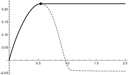
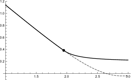
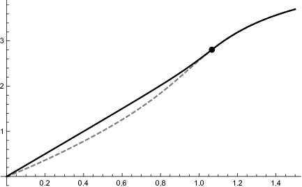
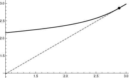
Figure 2: Numerical results under the exponential OU model (31): (a) Plots of function H⁡(z)H(z) (dashed gray) and Hf​(z)H_{f}(z) (solid black). The “pasting point” ψq​(bf⋆)=1.0674\psi_{q}(b_{f}^{\star})=1.0674 is indicated by the black dot. (b) Plots of the reward function h⁡(x)h(x) (dashed gray) and the value function vf​(x,x)v_{f}(x,x) (solid black). The “pasting point” is bf⋆=2.8845b_{f}^{\star}=2.8845 (black dot). (c) Plots of the reward function H(1)​(z)H^{(1)}(z) (dashed gray) and its smallest concave majorant (solid black), along with the “pasting point” z¯f⋆=0.5441\bar{z}_{f}^{\star}=0.5441 (black dot). (d) Plots of the reward function vf​(x,x)−hb​(x)v_{f}(x,x)-h_{b}(x) (dashed gray) and the value function vf(1)​(x)v_{f}^{(1)}(x) (solid black), and the “pasting point” b¯f⋆=1.9488\underline{b}_{f}^{\star}=1.9488 (black dot).

5.1 Value Function and Optimal Strategy

Upon purchasing of the asset, we set a percentage drawdown trailing stop, i.e. f⁡(x)=(1−α)​xf(x)=(1-\alpha)x, where α∈(0,1)\alpha\in(0,1) is a constant.

In this study, we select the following parameter values:

λ=0.6,θ=1,σ=0.2,q=0.05,c0=0.02,α=0.3.\displaystyle\lambda=0.6,\theta=1,\sigma=0.2,q=0.05,c_{0}=0.02,\alpha=0.3. (32)

This means that we will liquidate the asset whenever its price drops from its running maximum since the acquisition by more than 30%30\%.

In Figure 2(a), we plot the function H⁡(⋅)H(\cdot) defined as in (27). We also have plotted the function Hf​(⋅)H_{f}(\cdot) defined as in (23) (see also (29)), which is obtained by first solving equation (21) with f⁡(x)=(1−α)​xf(x)=(1-\alpha)x for bf⋆(=2.8845)b_{f}^{\star}(=2.8845), and then using ODE (29) to numerically obtain Hf​(⋅)H_{f}(\cdot). We notice that, in contrast to the value function for a fixed stop-loss level (Theorem 3.1, see also Leung and Li (2015)), the function Hf​(⋅)H_{f}(\cdot) is not concave over (0,ψq​(bf⋆))(0,\psi_{q}(b_{f}^{\star})). This is because, although ϕq−​(x)​Hf​(ψq​(x))=vf​(x,x)\phi_{q}^{-}(x)H_{f}(\psi_{q}(x))=v_{f}(x,x) is the value function for the optimal stopping problem (4) when x=x¯x=\bar{x}, it does not yield a martingale of (Xt,X¯t)(X_{t},\overline{X}_{t}), which requires using the function vf​(x,x¯)v_{f}(x,\bar{x}), not vf​(x,x)v_{f}(x,x).

In Figure 2(b), we plot the reward function h⁡(x)h(x) and the value function vf​(x,x)v_{f}(x,x) for the optimal liquidation problem (4) with x=x¯x=\bar{x}.

In Figure 2(c), we plot the function H(1)​(z)H^{(1)}(z) defined in (25) under the current exponential OU model. By checking the function’s derivative numerically, we conclude that it is concave to the left of its maximum point. Hence, the smallest concave majorant is given by

H^f,q(1)​(z)=H(1)​(z∧z¯f⋆),∀z∈ℝ+.\hat{H}_{f,q}^{(1)}(z)=H^{(1)}(z\wedge\overline{z}_{f}^{\star}),\quad\forall z\in\mathbb{R}_{+}.

Therefore, in this case, the optimal acquisition strategy is to purchase the asset once the price is lower than b¯f⋆=1.9488\underline{b}_{f}^{\star}=1.9488.

In Figure 2(d), we plot the function vf​(x,x)−hb​(x)v_{f}(x,x)-h_{b}(x) and the value function vf(1)​(x)v_{f}^{(1)}(x) for the optimal acquisition problem (8), and the “pasting point” is at ψq−1​(z¯f⋆)=1.9488\psi_{q}^{-1}(\bar{z}_{f}^{\star})=1.9488.

In summary, for the exponential OU model (31) with parameters as given in (32), the optimal trading strategy is to purchase the asset when price is lower than ψq−1​(z¯f⋆)=1.9488\psi_{q}^{-1}(\bar{z}_{f}^{\star})=1.9488, and setup the 30%30\% trailing stop order as an exit plan, and then wait until either the trailing stop is being activated or the price reaches target bf⋆=2.8845b_{f}^{\star}=2.8845.

Refer to caption
Figure 3: Earlier liquidation premium (black) pf​(x,x)p_{f}(x,x) and function x−f⁡(x)=α​xx-f(x)=\alpha x (dashed) under the exponential OU model (31).

Lastly, in Figure 3 we plot the early liquidation premium of ρf∧τX+​(bf⋆)\rho_{f}\wedge\tau_{X}^{+}(b_{f}^{\star}) over the plain trailing stop ρf\rho_{f} when x=x¯x=\bar{x}. This measure the “value” of our result in problem (4). By Corollary 4.2, we know that, for each x∈Ix\in I,

pf​(x,x)=exp⁡(∫xbf⋆∨x−ψq′​(u)​d​uψq​(u)−ψq​(f⁡(u)))​(h⁡(bf⋆∨x)−gf​(bf⋆∨x,bf⋆∨x)).p_{f}(x,x)=\exp(\int_{x}^{b_{f}^{\star}\vee x}\frac{-\psi_{q}^{\prime}(u)\textup{d}u}{\psi_{q}(u)-\psi_{q}(f(u))})\left(h(b_{f}^{\star}\vee x)-g_{f}(b_{f}^{\star}\vee x,b_{f}^{\star}\vee x)\right). (33)

To numerically evaluate (33), we use the fusion of a “limiting order” τX+​(b)\tau_{X}^{+}(b) and the trailing stop ρf\rho_{f}, with bb chosen sufficiently large so that

𝔼x(e−q⁡(τX+​(b)∧ρf)𝟏{τX+(b)<ρf})<0.005,\displaystyle\mathbb{E}_{x}(\mathrm{e}^{-q(\tau_{X}^{+}(b)\wedge\rho_{f})}\mathbf{1}_{\{\tau_{X}^{+}(b)<\rho_{f}\}})<0.005,
0<h(b)𝔼x(e−q⁡(τX+​(b)∧ρf)𝟏{τX+(b)<ρf})<0.03,\displaystyle 0<h(b)\mathbb{E}_{x}(\mathrm{e}^{-q(\tau_{X}^{+}(b)\wedge\rho_{f})}\mathbf{1}_{\{\tau_{X}^{+}(b)<\rho_{f}\}})<0.03,

for all xx in the plotting region of Figure 3. Then gf​(x,x)g_{f}(x,x) is approximated by the value of this strategy, which is subsequently solved using an ODE similar as (30).

In Figure 3, we compare the early liquidation premium pf​(x,x)p_{f}(x,x) with the function x−f⁡(x)=α​xx-f(x)=\alpha x (α=0.3\alpha=0.3), which is the maximum loss of the trailing stop order if the price XX reaches the trailing floor immediately (but without an overshoot). We notice that, for large xx, the gain from our strategy over the plain trailing stop approaches 30% of the price level. Take into account of discounting and transaction costs, this example suggests that setting a trailing stop when the asset price is high will almost always incur a 30% loss at exit.

5.2 Sensitivity Analysis and Financial Interpretations

The following illustrative numerical examples will shed light on the sensitivity of the optimal acquisition and liquidation thresholds, b¯f⋆\underline{b}_{f}^{\star} and bf⋆b_{f}^{\star}, with respect to the trailing stop level α\alpha, and transaction cost c0c_{0}. This involve numerical computation of the thresholds, as well as the critical level where function (ℒ−q)​h​(x)(\mathcal{L}-q)h(x) vanishes.

Refer to caption
(a) (bf⋆,x0,b¯f⋆)(b_{f}^{\star},x_{0},\underline{b}_{f}^{\star}) vs. α\alpha
Refer to caption
(b) (bf⋆,x0,b¯f⋆)(b_{f}^{\star},x_{0},\underline{b}_{f}^{\star}) vs. σ\sigma
Refer to caption
(c) (bf⋆,x0,b¯f⋆)(b_{f}^{\star},x_{0},\underline{b}_{f}^{\star}) vs. λ\lambda
Refer to caption
(d) (bf⋆,x0,b¯f⋆)(b_{f}^{\star},x_{0},\underline{b}_{f}^{\star}) vs. c0c_{0}
Figure 4: Sensitivity of thresholds bf⋆b_{f}^{\star} (black), b¯f⋆\underline{b}_{f}^{\star} (gray), and the root x0x_{0} (red dashed) of (ℒ−q)​h​(x)=0(\mathcal{L}-q)h(x)=0, under the exponential OU model (31): (a) Dependence on α∈[0.1,0.4]\alpha\in[0.1,0.4]; (b) Dependence of on σ∈[0.1,0.4]\sigma\in[0.1,0.4]; (c) Dependence of on λ∈[0.2,1.2]\lambda\in[0.2,1.2], and (d) Dependence of on c0∈[0,0.04]c_{0}\in[0,0.04]. In all figures, other parameters are set as in (32).

In Figure 4(a), we plot (bf⋆,x0,b¯f⋆)(b_{f}^{\star},x_{0},\underline{b}_{f}^{\star}) as a function of the trailing stop level α\alpha, with x0x_{0} (the dashed line) defined in Assumption 2.1. The optimal liquidation level bf⋆b_{f}^{\star} is increasing in α\alpha, confirming our result in Theorem 4.2. Moreover, the optimal acquisition level b¯f⋆\underline{b}_{f}^{\star} is also increasing in α\alpha. Recalling that a higher α\alpha means a lower trailing stop trigger, this means that a larger downside protection induces the investor to enter the market earlier. As seen in Figure 4(a), the investor with a higher α\alpha will acquire the asset at a price level closer to the critical level x0x_{0}. Our numerical results also suggest that, for small α\alpha, it may not be optimal to initiate the position at all, because the gain to be realized at the sell order at bf⋆b_{f}^{\star} or at the trailing stop will be too low compared to the transaction cost c0c_{0}. In such cases, we observe that supx∈ℝ(vf​(x,x)−h⁡(x))<c0=0.02\sup_{x\in\mathbb{R}}(v_{f}(x,x)-h(x))<c_{0}=0.02.

In Figure 4(b), we plot (bf⋆,x0,b¯f⋆)(b_{f}^{\star},x_{0},\underline{b}_{f}^{\star}) as a function of the asset’s volatility parameter σ\sigma. We see that, as σ\sigma increases, the optimal liquidation level increases, thanks to stronger force from the Brownian motion. However, the acquisition price level is lower for higher σ\sigma, which means that the investor is willing to establish a position at a lower price. However, higher volatility will increase the likelihood for the asset price to reach low levels earlier, so the actual entry time by the investor may be earlier or later. The decreasing pattern of b¯f⋆\underline{b}_{f}^{\star} with respect to σ\sigma suggests that the investor voluntarily lowers the take-profit level to mitigate the risk of realizing a reduced profit or a loss at the trailing stop in a more volatile market.

Figure 4(c) illustrates the effect of the asset’s rate of mean reversion λ\lambda. A higher λ\lambda means that the log-price will move around its long-term mean θ\theta faster. As a response, the investor enters the market earlier at a higher entry level and exit at a lower level, resulting in a quick roundtrip, as reflected in the plot by the increasing trends of bf⋆b_{f}^{\star} and b¯f⋆\underline{b}_{f}^{\star} with respect to λ\lambda. Moreover, their distance is shrinking as λ\lambda continues to increase. Intuitively, since the asset price tends to rapidly revert to the mean, it does not make sense to select entry and exit price levels that are far apart and away from the mean as the chance of execution is too low.

The effect of transaction cost c0c_{0} is shown in Figure 4(d), where we plot (bf⋆,x0,b¯f⋆)(b_{f}^{\star},x_{0},\underline{b}_{f}^{\star}) as a function of c0c_{0}. The optimal liquidation level bf⋆b_{f}^{\star} increases slightly with respect to c0c_{0} while the optimal acquisition level b¯f⋆\underline{b}_{f}^{\star} decreases in c0c_{0}. To interpret, higher transaction costs discourage both acquisition and liquidation, though the effect is not significant. Nevertheless, as pointed out in our analysis above, while there is always a finite optimal liquidation price bf⋆b_{f}^{\star} given any transaction cost, a high transaction cost may make the trade unprofitable and thus exclude market entry.

Appendix A Proofs

Proof of Lemma 2.2.

Following Dayanik and Karatzas (2003), let us define For any b∈Ib\in I, let us define

H⁡(z):=h⁡(x)ϕq−​(x), where ​z=ψq​(x)∈ℝ+.H(z):=\frac{h(x)}{\phi_{q}^{-}(x)},\text{ where }z=\psi_{q}(x)\in\mathbb{R}_{+}. (34)

By (Dayanik and Karatzas, 2003, Proposition 5.11), we know that the value function

V(x):=supτ∈𝒯𝔼x(e−r​τh(Xτ)𝟏{τ<∞}),V(x):=\sup_{\tau\in\mathcal{T}}\mathbb{E}_{x}(\mathrm{e}^{-r\tau}h(X_{\tau})\mathbf{1}_{\{\tau<\infty\}}),

is given by ϕq−​(x)​H^​(ψq​(x))\phi_{q}^{-}(x)\hat{H}(\psi_{q}(x)), where H^​(⋅)\hat{H}(\cdot) is the smallest nonnegative concave majorant of H⁡(⋅)H(\cdot) on ℝ+\mathbb{R}_{+}. On the other hand, by (Dayanik and Karatzas, 2003, Section 6), we have

H′′​(z)=2σ2​(x)​ϕq−​(x)​(ψq′​(x))2​((ℒ−q)​h​(x)),for ​z=ψq​(x).H^{\prime\prime}(z)=\frac{2}{\sigma^{2}(x)\phi_{q}^{-}(x)(\psi_{q}^{\prime}(x))^{2}}\left((\mathcal{L}-q)h(x)\right),\quad\text{for }z=\psi_{q}(x).

So Assumption 2.1 implies that H⁡(⋅)H(\cdot) is convex on (0,ψq​(x0))(0,\psi_{q}(x_{0})), and concave on (ψq​(x0),∞)(\psi_{q}(x_{0}),\infty). We now examine the behavior of H⁡(⋅)H(\cdot) near 0 and ∞\infty. From (34) we know that,

  1. 1.

    if h⁡(l+)≥0h(l+)\geq 0, then h⁡(l+)h(l+) is finite, and H⁡(0+)=limx↓lh⁡(x)ϕq−​(x)=0H(0+)=\lim_{x\downarrow l}\frac{h(x)}{\phi_{q}^{-}(x)}=0;

  2. 2.

    if h⁡(l+)<0h(l+)<0, then H⁡(z)<0H(z)<0 for sufficiently small z>0z>0.

Moreover, from

F⁡(z):=H⁡(z)z=h⁡(x)ϕq+​(x), where ​z=ψq​(x)F(z):=\frac{H(z)}{z}=\frac{h(x)}{\phi_{q}^{+}(x)},\text{ where }z=\psi_{q}(x)

we know H⁡(z)>0H(z)>0 for sufficiently large z>0z>0. Here, function F⁡(⋅)F(\cdot) is twice continuously differentiable on ℝ+\mathbb{R}_{+}, and by Assumption 2.1 we know that supz≥ψq​(x0)F⁡(z)=F⁡(z∗)\sup_{z\geq\psi_{q}(x_{0})}F(z)=F(z_{*}) for some z∗∈[ψq​(x0),∞)z_{*}\in[\psi_{q}(x_{0}),\infty). Obviously F⁡(z∗)>0F(z_{*})>0, which implies that H⁡(z)=h⁡(x)ϕq−​(x)>0H(z)=\frac{h(x)}{\phi_{q}^{-}(x)}>0 for all z>z∗z>z_{*} since h⁡(⋅)h(\cdot) is monotone. Furthermore, z∗z_{*} must satisfy the first order condition

1z∗​(H′​(z∗)−F⁡(z∗))=0.\frac{1}{z_{*}}(H^{\prime}(z_{*})-F(z_{*}))=0. (35)

Now define function

H~(z)=F(z∗)z𝟏{z<z∗}+H(z)𝟏{z≥z∗},\tilde{H}(z)=F(z_{*})z\mathbf{1}_{\{z<z_{*}\}}+H(z)\mathbf{1}_{\{z\geq z_{*}\}},

which is clearly continuously differentiable and concave on ℝ+\mathbb{R}_{+}, thanks to (35). Function H~​(⋅)\tilde{H}(\cdot) is also positive on ℝ+\mathbb{R}_{+}, which is evident from the construction. Hence we conclude that H~​(⋅)\tilde{H}(\cdot) is the smallest concave majorant of H⁡(⋅)H(\cdot). So the optimal stopping region is given by

ψq−1​({z∈ℝ+:H~​(z)=H⁡(z)})=(ψq−1​(z∗),r).\psi_{q}^{-1}(\{z\in\mathbb{R}_{+}:\tilde{H}(z)=H(z)\})=(\psi_{q}^{-1}(z_{*}),r).

Therefore, x⋆=ψq−1​(z∗)x^{\star}=\psi_{q}^{-1}(z_{*}) is the optimal stopping threshold. ∎

Proof of Proposition 3.1.

The proof is similar as that for Lemma 2.2. In the spirit of Dayanik and Karatzas (2003), we derive the optimal value function and the stopping region by constructing the smallest concave majorant of H⁡(z)H(z) on [ψq​(y),∞)[\psi_{q}(y),\infty). By the convexity of H⁡(⋅)H(\cdot), we know this concave majorant is given by

H^y​(z)={H⁡(ψq​(y))​z⁡(y)−zz​(y)−ψq​(y)+H⁡(z⁡(y))​z−ψq​(y)z​(y)−ψq​(y),∀z∈(ψq​(y),z⁡(y)),H⁡(z),∀z∉(ψq​(y),z⁡(y)),\hat{H}_{y}(z)=\begin{cases}H(\psi_{q}(y))\frac{z(y)-z}{z(y)-\psi_{q}(y)}+H(z(y))\frac{z-\psi_{q}(y)}{z(y)-\psi_{q}(y)},&\forall z\in(\psi_{q}(y),z(y)),\\ H(z),&\forall z\not\in(\psi_{q}(y),z(y)),\end{cases} (36)

where z⁡(y)z(y) is defined as

z⁡(y):=infarg⁡maxz>ψq​(x0)⁡H⁡(z)−H⁡(ψq​(y))z−ψq​(y).z(y):=\inf\mathop{\arg\max}_{z>\psi_{q}(x_{0})}\frac{H(z)-H(\psi_{q}(y))}{z-\psi_{q}(y)}. (37)

Thus, the optimal stopping region is given by

𝒮y𝖲,𝖫=ψq−1​(ℝ+\(ψq​(y),z⁡(y)))=(l,y]∪[ψq−1​(z⁡(y)),r).\mathcal{S}_{y}^{\sf S,L}=\psi_{q}^{-1}(\mathbb{R}_{+}\backslash(\psi_{q}(y),z(y)))=(l,y]\cup[\psi_{q}^{-1}(z(y)),r).

Therefore, the optimal stopping barrier is given by b⁡(y):=ψq−1​(z⁡(y))b(y):=\psi_{q}^{-1}(z(y)).

From Remark 3.1 we know that, for l≤y1<y2<x0l\leq y_{1}<y_{2}<x_{0}, the equalities hold:

((l,y1]∪[b⁡(y1),r))≡𝒮y1𝖲,𝖫⊂𝒮y2𝖲,𝖫≡((l,y2]∪[b⁡(y2),r)).\left((l,y_{1}]\cup[b(y_{1}),r)\right)\equiv\mathcal{S}_{y_{1}}^{\sf S,L}\subset\mathcal{S}_{y_{2}}^{\sf S,L}\equiv\left((l,y_{2}]\cup[b(y_{2}),r)\right).

Thus necessarily, b⁡(y2)≤b⁡(y1)≤b⁡(l)=x∗<rb(y_{2})\leq b(y_{1})\leq b(l)=x_{*}<r. Because z⁡(y)z(y) is an interior maximizer in the objective function in (37), it must satisfy the first order condition:

1z​(y)−ψq​(y)​(H′​(z⁡(y))−H⁡(z⁡(y))−H⁡(ψq​(y))z​(y)−ψq​(y))=0.\frac{1}{z(y)-\psi_{q}(y)}\bigg(H^{\prime}(z(y))-\frac{H(z(y))-H(\psi_{q}(y))}{z(y)-\psi_{q}(y)}\bigg)=0. (38)

This gives (20).

As y↑x0y\uparrow x_{0}, b⁡(y)b(y) converges to some limit in [x0,r)[x_{0},r). Suppose that b⁡(x0−)≡b¯>x0b(x_{0}-)\equiv\underline{b}>x_{0}, then the concavity of H⁡(⋅)H(\cdot) over (ψq​(x0),∞)(\psi_{q}(x_{0}),\infty) implies that

H′​(ψq​(b¯))≤H⁡(ψq​(b¯))−H⁡(ψq​(x0))ψq​(b¯)−ψq​(x0).H^{\prime}(\psi_{q}(\underline{b}))\leq\frac{H(\psi_{q}(\underline{b}))-H(\psi_{q}(x_{0}))}{\psi_{q}(\underline{b})-\psi_{q}(x_{0})}.

However, taking limit in (38) as y↑x0y\uparrow x_{0}, we know that the above inequality is in fact an equality. This, together with the concavity of H⁡(⋅)H(\cdot) implies that H⁡(⋅)H(\cdot) is in fact a straight line over [ψq​(x0),ψq​(b¯)][\psi_{q}(x_{0}),\psi_{q}(\underline{b})], but then (by the definition of z⁡(y)z(y), again) we must have b⁡(x0−)=x0b(x_{0}-)=x_{0} instead.

We use implicit differentiation to prove b⁡(y)b(y) is strictly decreasing and differentiable on (l,x0)(l,x_{0}). To that end, we denote z=z⁡(y)z=z(y) and u=ψq​(y)u=\psi_{q}(y), then the first order equation in (38) reads as

f⁡(z,u)=0, where ​f​(z,w)=H′​(z)−H⁡(z)−H⁡(u)z−u.f(z,u)=0,\text{ where }f(z,w)=H^{\prime}(z)-\frac{H(z)-H(u)}{z-u}.

By the definition of z≡z⁡(y)z\equiv z(y) we have

∂f∂u\displaystyle\frac{\partial f}{\partial u} =H′​(u)−H⁡(z)−H⁡(u)(z−u)<0,\displaystyle=H^{\prime}(u)-\frac{H(z)-H(u)}{(z-u)}<0,
∂f∂z\displaystyle\frac{\partial f}{\partial z} =H′′​(z)−1z−u​f​(z,u)=H′′​(z)<0.\displaystyle=H^{\prime\prime}(z)-\frac{1}{z-u}f(z,u)=H^{\prime\prime}(z)<0.

Thus, we know that z⁡(y)z(y) is strictly decreasing and differentiable in ψq​(y)\psi_{q}(y). In order words, z⁡(y)z(y) is differentiable in yy and z′​(y)<0z^{\prime}(y)<0 for any y∈(l,x0)y\in(l,x_{0}). ∎

Proof of Corollary 4.1.

From Theorem 3.1 we know that x¯↦b⁡(f⁡(x¯))\bar{x}\mapsto b(f(\bar{x})) is strictly decreasing and continuous over (f−1​(l),f−1​(x0))(f^{-1}(l),f^{-1}(x_{0})), and the mapping x¯:↦x¯\bar{x}:\mapsto\bar{x} is strictly increasing over the same domain. Therefore, the difference D⁡(x¯):=b⁡(f⁡(x¯))−x¯D(\bar{x}):=b(f(\bar{x}))-\bar{x} is strictly decreasing, and D⁡(x¯)≥D⁡(x0)>0D(\bar{x})\geq D(x_{0})>0 for all x¯∈(f−1​(l),x0]\bar{x}\in(f^{-1}(l),x_{0}], and by Proposition 3.1,

limx¯↑f−1​(x0)D⁡(x¯)=x0−f−1​(x0)<0.\lim_{\bar{x}\uparrow f^{-1}(x_{0})}D(\bar{x})=x_{0}-f^{-1}(x_{0})<0.

As a consequence, we can define bf⋆:=inf{x¯<f−1​(x0):D⁡(x¯)≤0}b_{f}^{\star}:=\inf\{\bar{x}<f^{-1}(x_{0}):D(\bar{x})\leq 0\}, and bf⋆∈(x0,f−1​(x0))b_{f}^{\star}\in(x_{0},f^{-1}(x_{0})), so f⁡(bf⋆)≤x0f(b_{f}^{\star})\leq x_{0}.

Now for all x¯<bf⋆\bar{x}<b_{f}^{\star}, by the construction of bf⋆b_{f}^{\star} we have b⁡(f⁡(x¯))>x¯b(f(\bar{x}))>\bar{x}, by definition of z⁡(f⁡(x¯))≡ψq​(b⁡(f⁡(x¯)))z(f(\bar{x}))\equiv\psi_{q}(b(f(\bar{x}))) in the proof of Proposition 3.1 we know that z⁡(f⁡(x¯))>ψq​(x¯)z(f(\bar{x}))>\psi_{q}(\bar{x}). Because the line segment l0l_{0} connecting (ψq​(f⁡(x¯)),H⁡(ψq​(f⁡(x¯))))(\psi_{q}(f(\bar{x})),H(\psi_{q}(f(\bar{x})))) and (z⁡(f⁡(x¯)),H⁡(ψq​(f⁡(x¯))))(z(f(\bar{x})),H(\psi_{q}(f(\bar{x})))) gives part of the concave majorant of H⁡(⋅)H(\cdot), we know that the line segment l1l_{1} connecting (ψq​(f⁡(x¯)),H⁡(ψq​(f⁡(x¯))))(\psi_{q}(f(\bar{x})),H(\psi_{q}(f(\bar{x})))) and (ψq​(x¯),H⁡(ψq​(x¯)))(\psi_{q}(\bar{x}),H(\psi_{q}(\bar{x}))), which is below line segment l0l_{0}, must go below the graph of H⁡(⋅)H(\cdot) at ψq​(x¯)\psi_{q}(\bar{x}). This implies that the derivative of H⁡(⋅)H(\cdot) at ψq​(x¯)\psi_{q}(\bar{x}) must be strictly greater than that of line segment l1l_{1}. That is,

H′(ψq(x¯))>H⁡(ψq​(x¯))−H⁡(ψq​(f⁡(x¯)))ψq​(x¯)−ψq​(f⁡(x¯))⇔Γ(x¯)>0.H^{\prime}(\psi_{q}(\bar{x}))>\frac{H(\psi_{q}(\bar{x}))-H(\psi_{q}(f(\bar{x})))}{\psi_{q}(\bar{x})-\psi_{q}(f(\bar{x}))}\quad\Leftrightarrow\quad\Gamma(\bar{x})>0.

On the other hand, for all f−1​(x0)>x¯>bf⋆f^{-1}(x_{0})>\bar{x}>b_{f}^{\star}, we have b⁡(f⁡(x¯))<x¯b(f(\bar{x}))<\bar{x}. Using similar argument as above, we know that z⁡(f⁡(x¯))=ψq​(b⁡(f⁡(x¯)))<ψq​(x¯)z(f(\bar{x}))=\psi_{q}(b(f(\bar{x})))<\psi_{q}(\bar{x}). Since the line segment l1l_{1} connecting (ψq​(f⁡(x¯)),H⁡(ψq​(f⁡(x¯))))(\psi_{q}(f(\bar{x})),H(\psi_{q}(f(\bar{x})))) and (ψq​(x¯),H⁡(ψq​(x¯)))(\psi_{q}(\bar{x}),H(\psi_{q}(\bar{x}))) is a line segment connecting two points on the graph of a concave function H^​(⋅)\hat{H}(\cdot), which is the smallest concave majorant of H⁡(⋅)H(\cdot) over [ψq​(f​(x¯)),∞)[\psi_{q}(f(\bar{x})),\infty), we know that

H^′(ψq(x¯))=H′(ψq(x¯))<H⁡(ψq​(x¯))−H⁡(ψq​(f⁡(x¯)))ψq​(x¯)−ψq​(f⁡(x¯))⇔Γ(x¯)<0.\hat{H}^{\prime}(\psi_{q}(\bar{x}))=H^{\prime}(\psi_{q}(\bar{x}))<\frac{H(\psi_{q}(\bar{x}))-H(\psi_{q}(f(\bar{x})))}{\psi_{q}(\bar{x})-\psi_{q}(f(\bar{x}))}\quad\Leftrightarrow\quad\Gamma(\bar{x})<0.

Expressing H⁡(⋅)H(\cdot) and its derivative with h⁡(⋅),ϕq−​(⋅),ψq​(⋅)h(\cdot),\phi_{q}^{-}(\cdot),\psi_{q}(\cdot) and their derivatives yields (21) and completes the proof. ∎

Proof of Lemma 4.1.

Let us denote by 𝐞q\mathbf{e}_{q} an exponential random variable with mean 1/q1/q, which is independent of XX. Then we notice that

𝔼x¯,x¯(e−q​ρfh(Xρf)𝟏{τX+(b)<ρf})=\displaystyle\mathbb{E}_{\bar{x},\bar{x}}(\mathrm{e}^{-q\rho_{f}}h(X_{\rho_{f}})\mathbf{1}_{\{\tau_{X}^{+}(b)<\rho_{f}\}})= 𝔼x¯,x¯(h(Xρf)𝟏{ρf<τX+(b)∧𝐞q}),\displaystyle\mathbb{E}_{\bar{x},\bar{x}}(h(X_{\rho_{f}})\mathbf{1}_{\{\rho_{f}<\tau_{X}^{+}(b)\wedge\mathbf{e}_{q}\}}),
𝔼x¯,x¯(e−q​τX+​(b)𝟏{τX+(b)<ρf})=\displaystyle\mathbb{E}_{\bar{x},\bar{x}}(\mathrm{e}^{-q\tau_{X}^{+}(b)}\mathbf{1}_{\{\tau_{X}^{+}(b)<\rho_{f}\}})= ℙx¯,x¯​(τX+​(b)<ρf∧𝐞q).\displaystyle\mathbb{P}_{\bar{x},\bar{x}}(\tau_{X}^{+}(b)<\rho_{f}\wedge\mathbf{e}_{q}).

To calculate the right-hand sides of the above, we consider an excursion of XX below uu (notice that τX+​(u−)=inf{t>0:Xt≥u}\tau_{X}^{+}(u-)=\inf\{t>0:X_{t}\geq u\} is the first hitting time of XX to uu):

ϵu={ϵu(s):=XτX+​(u−)−XτX+​(u−)+s}0<s≤τX+​(u)−τX+​(u−),\epsilon_{u}=\{\epsilon_{u}(s):=X_{\tau_{X}^{+}(u-)}-X_{\tau_{X}^{+}(u-)+s}\}_{0<s\leq\tau_{X}^{+}(u)-\tau_{X}^{+}(u-)},

which is defined for all u≥X0=X¯0=x¯u\geq X_{0}=\overline{X}_{0}=\bar{x} such that its lifetime ζ⁡(ϵu):=τX+​(u)−τX+​(u−)>0\zeta(\epsilon_{u}):=\tau_{X}^{+}(u)-\tau_{X}^{+}(u-)>0. When ζ⁡(ϵu)=0\zeta(\epsilon_{u})=0 we set ϵu=∂\epsilon_{u}=\partial, an isolated point. Then the process {(u,ϵu)}u≥x¯\{(u,\epsilon_{u})\}_{u\geq\bar{x}} is a Poisson point process with jump measure d​u×d​nu\textup{d}u\times\textup{d}n_{u}, where nun_{u} is the excursion measure for ϵu\epsilon_{u}. Define Tf​(ϵu):=inf{0<s<ζ⁡(ϵu):ϵu​(s)>u−f⁡(u)}T_{f}(\epsilon_{u}):=\inf\{0<s<\zeta(\epsilon_{u}):\epsilon_{u}(s)>u-f(u)\}. It is known from Salminen et al. (2007) and Lemma 2.1 that,

nu​(𝐞q<ζ⁡(ϵu)∧Tf​(ϵu))=\displaystyle n_{u}(\mathbf{e}_{q}<\zeta(\epsilon_{u})\wedge T_{f}(\epsilon_{u}))= limx↑u1u−x(1−𝔼x(e−q​τX+​(u)𝟏{τX+(u)<τX−(f(u))}))−limx↑u𝔼x(e−q​τX−​(f⁡(u))𝟏{τX−(f(u))<τX+(u)})u−x\displaystyle\lim_{x\uparrow u}\frac{1}{u-x}\left(1-\mathbb{E}_{x}(\mathrm{e}^{-q\tau_{X}^{+}(u)}\mathbf{1}_{\{\tau_{X}^{+}(u)<\tau_{X}^{-}(f(u))\}})\right)-\lim_{x\uparrow u}\frac{\mathbb{E}_{x}(\mathrm{e}^{-q\tau_{X}^{-}(f(u))}\mathbf{1}_{\{\tau_{X}^{-}(f(u))<\tau_{X}^{+}(u)\}})}{u-x}
=\displaystyle= ϕq−,′(u)ϕq−​(u)+(1−ϕq−​(u)ϕq−​(f⁡(u)))​ψq′​(u)ψq​(u)−ψq​(f⁡(u)),\displaystyle\frac{\phi_{q}^{-,\prime}(u)}{\phi_{q}^{-}(u)}+\bigg(1-\frac{\phi_{q}^{-}(u)}{\phi_{q}^{-}(f(u))}\bigg)\frac{\psi_{q}^{\prime}(u)}{\psi_{q}(u)-\psi_{q}(f(u))},
nu​(Tf​(ϵu)<ζ⁡(ϵu)∧𝐞q)=\displaystyle n_{u}(T_{f}(\epsilon_{u})<\zeta(\epsilon_{u})\wedge\mathbf{e}_{q})= limx↑u𝔼x(e−q​τX−​(f⁡(u))𝟏{τX−(f(u))<τX+(u)})u−x=ϕq−​(u)ϕq−​(f⁡(u))​ψq′​(u)ψq​(u)−ψq​(f⁡(u)).\displaystyle\lim_{x\uparrow u}\frac{\mathbb{E}_{x}(\mathrm{e}^{-q\tau_{X}^{-}(f(u))}\mathbf{1}_{\{\tau_{X}^{-}(f(u))<\tau_{X}^{+}(u)\}})}{u-x}=\frac{\phi_{q}^{-}(u)}{\phi_{q}^{-}(f(u))}\frac{\psi_{q}^{\prime}(u)}{\psi_{q}(u)-\psi_{q}(f(u))}.

Hence,

nu​(𝐞q<ζ⁡(ϵu)∧Tf​(ϵu)​ or ​Tf​(ϵu)<ζ⁡(ϵu)∧𝐞q)=ϕq−,′(u)ϕq−​(u)−ψq′​(u)ψq​(u)−ψq​(f⁡(u)).n_{u}(\mathbf{e}_{q}<\zeta(\epsilon_{u})\wedge T_{f}(\epsilon_{u})\text{ or }T_{f}(\epsilon_{u})<\zeta(\epsilon_{u})\wedge\mathbf{e}_{q})=\frac{\phi_{q}^{-,\prime}(u)}{\phi_{q}^{-}(u)}-\frac{\psi_{q}^{\prime}(u)}{\psi_{q}(u)-\psi_{q}(f(u))}.

Let AA be the space of all excursions ϵu\epsilon_{u} such that Tf​(ϵu)<ζ⁡(ϵu)∧𝐞qT_{f}(\epsilon_{u})<\zeta(\epsilon_{u})\wedge\mathbf{e}_{q}, and BB be the space of all excursions ϵu\epsilon_{u} such that 𝐞q<ζ⁡(ϵu)∧Tf​(ϵu)\mathbf{e}_{q}<\zeta(\epsilon_{u})\wedge T_{f}(\epsilon_{u}). We have that A∩B=∅A\cap B=\emptyset. Consider a Poisson process (with time indexed by the running maximum X¯\overline{X}) that jumps whenever the current excursion ϵX¯∈A∪B\epsilon_{\overline{X}}\in A\cup B, then from the above calculation, we know that this Poisson process has jump intensity nu​(𝐞q<ζ⁡(ϵu)∧Tf​(ϵu)​ or ​Tf​(ϵu)<ζ⁡(ϵu)∧𝐞q)n_{u}(\mathbf{e}_{q}<\zeta(\epsilon_{u})\wedge T_{f}(\epsilon_{u})\text{ or }T_{f}(\epsilon_{u})<\zeta(\epsilon_{u})\wedge\mathbf{e}_{q}). So ℙx¯,x¯​(τX+​(b)<ρf∧𝐞q)\mathbb{P}_{\bar{x},\bar{x}}(\tau_{X}^{+}(b)<\rho_{f}\wedge\mathbf{e}_{q}) is the same as the probability that this Poisson process has no jump over [x¯,b)[\bar{x},b), which is given by

exp(−∫x¯bnu(𝐞q<ζ(ϵu)∧Tf(ϵu) or Tf(ϵu)<ζ(ϵu)∧𝐞q)du)=\displaystyle\exp(-\int_{\bar{x}}^{b}n_{u}(\mathbf{e}_{q}<\zeta(\epsilon_{u})\wedge T_{f}(\epsilon_{u})\text{ or }T_{f}(\epsilon_{u})<\zeta(\epsilon_{u})\wedge\mathbf{e}_{q})\textup{d}u)= ϕq−​(x¯)ϕq−​(b)exp(−∫x¯bψq′​(u)​d​uψq​(u)−ψq​(f⁡(u))).\displaystyle\frac{\phi_{q}^{-}(\bar{x})}{\phi_{q}^{-}(b)}\exp(-\int_{\bar{x}}^{b}\frac{\psi_{q}^{\prime}(u)\textup{d}u}{\psi_{q}(u)-\psi_{q}(f(u))}).

Moreover, for any v∈[x¯,b)v\in[\bar{x},b), the probability that the Poisson process will have the first jump at “time” d​v\textup{d}v as a result of ϵv∈A\epsilon_{v}\in A, is given by

exp(−∫x¯vnu(𝐞q<ζ(ϵu)∧Tf(ϵu) or Tf(ϵu)<ζ(ϵu)∧𝐞q)du)⋅nv(Tf(ϵv)<ζ(ϵv)∧𝐞q)dv\displaystyle\exp(-\int_{\bar{x}}^{v}n_{u}(\mathbf{e}_{q}<\zeta(\epsilon_{u})\wedge T_{f}(\epsilon_{u})\text{ or }T_{f}(\epsilon_{u})<\zeta(\epsilon_{u})\wedge\mathbf{e}_{q})\textup{d}u)\cdot n_{v}(T_{f}(\epsilon_{v})<\zeta(\epsilon_{v})\wedge\mathbf{e}_{q})\textup{d}v
=\displaystyle= ϕq−​(x¯)ϕq−​(v)exp(−∫x¯vψq′​(u)​d​uψq​(u)−ψq​(f⁡(u)))×ϕq−​(v)ϕq−​(f⁡(v))ψq′​(v)ψq​(v)−ψq​(f⁡(v))dv\displaystyle\frac{\phi_{q}^{-}(\bar{x})}{\phi_{q}^{-}(v)}\exp(-\int_{\bar{x}}^{v}\frac{\psi_{q}^{\prime}(u)\textup{d}u}{\psi_{q}(u)-\psi_{q}(f(u))})\times\frac{\phi_{q}^{-}(v)}{\phi_{q}^{-}(f(v))}\frac{\psi_{q}^{\prime}(v)}{\psi_{q}(v)-\psi_{q}(f(v))}\textup{d}v
=\displaystyle= ϕq−​(x¯)ϕq−​(f⁡(v))ψq′​(v)ψq​(v)−ψq​(f⁡(v))exp(−∫x¯vψq′​(u)​d​uψq​(u)−ψq​(f⁡(u)))dv,\displaystyle\frac{\phi_{q}^{-}(\bar{x})}{\phi_{q}^{-}(f(v))}\frac{\psi_{q}^{\prime}(v)}{\psi_{q}(v)-\psi_{q}(f(v))}\exp(-\int_{\bar{x}}^{v}\frac{\psi_{q}^{\prime}(u)\textup{d}u}{\psi_{q}(u)-\psi_{q}(f(u))})\textup{d}v,

which is the same as ℙx¯,x¯​(X¯ρf∈d​v,ρf<τX+​(b)∧𝐞q)\mathbb{P}_{\bar{x},\bar{x}}(\overline{X}_{\rho_{f}}\in\textup{d}v,\rho_{f}<\tau_{X}^{+}(b)\wedge\mathbf{e}_{q}). The proof is complete by integrating in vv over [x¯,b)[\bar{x},b). ∎

Proof of Lemma 4.2.

Let us define for any b≥x¯b\geq\bar{x}

H¯(ψq(x¯),b):=H(ψq(b))exp(−∫x¯bψq′​(u)​d​uψq​(u)−ψq​(f⁡(u)))+∫x¯bψq′​(v)​H​(ψq​(f⁡(v)))w⁡(v)−w⁡(f⁡(v))exp(−∫x¯vψq′​(u)ψq​(u)−ψq​(f⁡(u))du)dv.\bar{H}(\psi_{q}(\bar{x}),b):=H(\psi_{q}(b))\exp(-\int_{\bar{x}}^{b}\frac{\psi_{q}^{\prime}(u)\,\textup{d}u}{\psi_{q}(u)-\psi_{q}(f(u))})\\ +\int_{\bar{x}}^{b}\frac{\psi_{q}^{\prime}(v)\,H(\psi_{q}(f(v)))}{w(v)-w(f(v))}\exp(-\int_{\bar{x}}^{v}\frac{\psi_{q}^{\prime}(u)}{\psi_{q}(u)-\psi_{q}(f(u))}\textup{d}u)\textup{d}v. (39)

It is clear that H¯​(ψq​(x¯),x¯)=H⁡(ψq​(x¯))=h⁡(x¯)ϕq−​(x¯)\bar{H}(\psi_{q}(\bar{x}),\bar{x})=H(\psi_{q}(\bar{x}))=\frac{h(\bar{x})}{\phi_{q}^{-}(\bar{x})}, and for b>x¯b>\bar{x} we have the right derivative of Hf​(ψq​(x¯),b)H_{f}(\psi_{q}(\bar{x}),b) in bb:

∂∂b​H¯​(ψq​(x¯),b)\displaystyle\frac{\partial}{\partial b}\bar{H}(\psi_{q}(\bar{x}),b)
=\displaystyle= ψq′(b)exp(−∫x¯bψq′​(u)​d​uψq​(u)−ψq​(f⁡(u)))(H+′(ψq(b))−H⁡(ψq​(b))−H⁡(ψq​(f⁡(b)))ψq​(b)−ψq​(f⁡(b))).\displaystyle\psi_{q}^{\prime}(b)\exp(-\int_{\bar{x}}^{b}\frac{\psi_{q}^{\prime}(u)\textup{d}u}{\psi_{q}(u)-\psi_{q}(f(u))})\bigg(H_{+}^{\prime}(\psi_{q}(b))-\frac{H(\psi_{q}(b))-H(\psi_{q}(f(b)))}{\psi_{q}(b)-\psi_{q}(f(b))}\bigg).

It follows that the sign of ∂∂b​H¯​(ψq​(x¯),b)\frac{\partial}{\partial b}\bar{H}(\psi_{q}(\bar{x}),b) depends on that of

Γ⁡(b)=H′​(ψq​(b))−H⁡(ψq​(b))−H⁡(ψq​(f⁡(b)))ψq​(b)−ψq​(f⁡(b)).\Gamma(b)=H^{\prime}(\psi_{q}(b))-\frac{H(\psi_{q}(b))-H(\psi_{q}(f(b)))}{\psi_{q}(b)-\psi_{q}(f(b))}.

But the latter is known to be positive for all b<bf⋆b<b_{f}^{\star}, thanks to Corollary 4.1. Because H′​(ψq​(⋅))H^{\prime}(\psi_{q}(\cdot)) is continuous, so is Γ⁡(⋅)\Gamma(\cdot). So we know that

uf​(x,x¯)ϕq−​(x)=\displaystyle\frac{u_{f}(x,\bar{x})}{\phi_{q}^{-}(x)}= H¯​(ψq​(x¯),bf⋆)=H⁡(ψq​(x¯))+∫x¯bf⋆∂∂u​H¯​(ψq​(x¯),u)​d​u>H⁡(ψq​(x¯))=h⁡(x)ϕq−​(x),∀x¯<bf⋆.\displaystyle\bar{H}(\psi_{q}(\bar{x}),b_{f}^{\star})=H(\psi_{q}(\bar{x}))+\int_{\bar{x}}^{b_{f}^{\star}}\frac{\partial}{\partial u}\bar{H}(\psi_{q}(\bar{x}),u)\textup{d}u>H(\psi_{q}(\bar{x}))=\frac{h(x)}{\phi_{q}^{-}(x)},\forall\bar{x}<b_{f}^{\star}.

This completes the proof. ∎

Proof of Corollary 4.2.

If f⁡(x¯)<x≤x¯<bf⋆f(\bar{x})<x\leq\bar{x}<b_{f}^{\star}, then by the strong Markov property of XX, we have

pf​(x,x¯)=\displaystyle p_{f}(x,\bar{x})= 𝔼x,x¯([e−q​τX+​(bf⋆)h(XτX+​(bf⋆))−e−q​ρfh(Xρf)]𝟏{τX+(bf⋆)<ρf<∞})\displaystyle\mathbb{E}_{x,\bar{x}}([\mathrm{e}^{-q\tau_{X}^{+}(b_{f}^{\star})}h(X_{\tau_{X}^{+}(b_{f}^{\star})})-\mathrm{e}^{-q\rho_{f}}h(X_{\rho_{f}})]\mathbf{1}_{\{\tau_{X}^{+}(b_{f}^{\star})<\rho_{f}<\infty\}})
=\displaystyle= 𝔼x,x¯(e−q​τX+​(bf⋆)𝟏{τX+(bf⋆)<ρf})(h(bf⋆)−𝔼bf⋆,bf⋆(e−q​ρfh(Xρf)𝟏{ρf<∞})),\displaystyle\mathbb{E}_{x,\bar{x}}(\mathrm{e}^{-q\tau_{X}^{+}(b_{f}^{\star})}\mathbf{1}_{\{\tau_{X}^{+}(b_{f}^{\star})<\rho_{f}\}})\,\left(h(b_{f}^{\star})-\mathbb{E}_{b_{f}^{\star},b_{f}^{\star}}(\mathrm{e}^{-q\rho_{f}}h(X_{\rho_{f}})\mathbf{1}_{\{\rho_{f}<\infty\}})\right),

where 𝔼bf⋆,bf⋆(e−q​ρfh(Xρf)𝟏{ρf<∞})=gf(bf⋆,bf⋆)\mathbb{E}_{b_{f}^{\star},b_{f}^{\star}}(\mathrm{e}^{-q\rho_{f}}h(X_{\rho_{f}})\mathbf{1}_{\{\rho_{f}<\infty\}})=g_{f}(b_{f}^{\star},b_{f}^{\star}) is given in Lemma 4.1, which is finite since we know that it is dominated from above by vf​(bf⋆,bf⋆)=h⁡(bf⋆)v_{f}(b_{f}^{\star},b_{f}^{\star})=h(b_{f}^{\star}). On the other hand, by the analysis in (22) and the results in Lemma 4.1, we have

𝔼x,x¯(e−q​τX+​(bf⋆)𝟏{τX+(bf⋆)<ρf})=\displaystyle\mathbb{E}_{x,\bar{x}}(\mathrm{e}^{-q\tau_{X}^{+}(b_{f}^{\star})}\mathbf{1}_{\{\tau_{X}^{+}(b_{f}^{\star})<\rho_{f}\}})= ϕq−​(x)ϕq−​(bf⋆)ψq​(x)−ψq​(f⁡(x¯))ψq​(x¯)−ψq​(f⁡(x¯))exp(−∫x¯bf⋆ψq′​(u)​d​uψq​(u)−ψq​(f⁡(u))).\displaystyle\frac{\phi_{q}^{-}(x)}{\phi_{q}^{-}(b_{f}^{\star})}\frac{\psi_{q}(x)-\psi_{q}(f(\bar{x}))}{\psi_{q}(\bar{x})-\psi_{q}(f(\bar{x}))}\exp(-\int_{\bar{x}}^{b_{f}^{\star}}\frac{\psi_{q}^{\prime}(u)\textup{d}u}{\psi_{q}(u)-\psi_{q}(f(u))}).

We obtain the claimed formula by combining the above results.

If f⁡(x¯)<x0f(\bar{x})<x_{0} and x¯≥bf⋆\bar{x}\geq b_{f}^{\star}, then from Theorem 3.1 and Theorem 4.1 we know that b⁡(f⁡(x¯))≤x¯b(f(\bar{x}))\leq\bar{x}, and for all f⁡(x¯)<x<b⁡(f⁡(x¯))f(\bar{x})<x<b(f(\bar{x})),

pf​(x,x¯)=\displaystyle p_{f}(x,\bar{x})= 𝔼x(e−q​τX+​(b⁡(f⁡(x¯)))𝟏{τX+(b(f(x¯)))<τX−(f(x¯))})(h(b(f(x¯)))−𝔼b⁡(f⁡(x¯),x¯CLOSE(e−q​ρfh(Xρf)𝟏{ρf<∞})).\displaystyle\mathbb{E}_{x}(\mathrm{e}^{-q\tau_{X}^{+}(b(f(\bar{x})))}\mathbf{1}_{\{\tau_{X}^{+}(b(f(\bar{x})))<\tau_{X}^{-}(f(\bar{x}))\}})\left(h(b(f(\bar{x})))-\mathbb{E}_{b(f(\bar{x}),\bar{x}}(\mathrm{e}^{-q\rho_{f}}h(X_{\rho_{f}})\mathbf{1}_{\{\rho_{f}<\infty\}})\right).

By using Lemma 2.1 we obtain that

𝔼x(e−q​τX+​(b⁡(f⁡(x¯)))𝟏{τX+(b(f(x¯)))<τX−(f(x¯))})=\displaystyle\mathbb{E}_{x}(\mathrm{e}^{-q\tau_{X}^{+}(b(f(\bar{x})))}\mathbf{1}_{\{\tau_{X}^{+}(b(f(\bar{x})))<\tau_{X}^{-}(f(\bar{x}))\}})= ϕq−​(x)ϕq−​(b⁡(f⁡(x¯)))​ψq​(x)−ψq​(f⁡(x¯))ψ⁡(b⁡(f⁡(x¯)))−ψq​(f⁡(x¯)).\displaystyle\frac{\phi_{q}^{-}(x)}{\phi_{q}^{-}(b(f(\bar{x})))}\frac{\psi_{q}(x)-\psi_{q}(f(\bar{x}))}{\psi(b(f(\bar{x})))-\psi_{q}(f(\bar{x}))}.

The claim in this case follows from Lemma 4.1.

In the last case that f⁡(x¯)<x0f(\bar{x})<x_{0}, x¯≥bf⋆\bar{x}\geq b_{f}^{\star} and b⁡(f⁡(x¯))≤x≤x¯b(f(\bar{x}))\leq x\leq\bar{x}, or f⁡(x¯)≥x0f(\bar{x})\geq x_{0} and f⁡(x¯)<x≤x¯f(\bar{x})<x\leq\bar{x}, from Theorem 3.1 and Theorem 4.1 we know that the optimal stopping rule for problem (4) is 0, so we have

pf(x,x¯)=h(x)−𝔼x,x¯(e−q​ρfh(Xρf)𝟏{ρf<∞}).p_{f}(x,\bar{x})=h(x)-\mathbb{E}_{x,\bar{x}}(\mathrm{e}^{-q\rho_{f}}h(X_{\rho_{f}})\mathbf{1}_{\{\rho_{f}<\infty\}}).

The completes the proof. ∎

Proof of Lemma 4.3.

The convexity of H⁡(⋅)H(\cdot) has already been proved in the proof of Lemma 2.2, so we only need to prove that for Hf​(⋅)H_{f}(\cdot). To that end, we recall (30) that

Hf′​(z)=Hf​(z)−H⁡(φ⁡(z))z−φ⁡(z),∀z∈(0,zf⋆),H_{f}^{\prime}(z)=\frac{H_{f}(z)-H(\varphi(z))}{z-\varphi(z)},\quad\forall z\in(0,z_{f}^{\star}),

from which we obtain that, for z∈(0,zf⋆)z\in(0,z_{f}^{\star}),

d​Hf′​(z)\displaystyle\textup{d}H_{f}^{\prime}(z) =Hf​(z)−H⁡(φ⁡(z))z−φ⁡(z)​d​z−H′​(φ⁡(z))​d​φ​(z)z−φ⁡(z)−Hf​(z)−H⁡(φ⁡(z))(z−φ⁡(z))2​(d​z−d​φ​(z))\displaystyle=\frac{\frac{H_{f}(z)-H(\varphi(z))}{z-\varphi(z)}\textup{d}z-H^{\prime}(\varphi(z))\textup{d}\varphi(z)}{z-\varphi(z)}-\frac{H_{f}(z)-H(\varphi(z))}{(z-\varphi(z))^{2}}(\textup{d}z-\textup{d}\varphi(z))
=(Hf​(z)−H⁡(φ⁡(z))z−φ⁡(z)−H′​(φ⁡(z)))​d​φ​(z)z−φ⁡(z)\displaystyle=\bigg(\frac{H_{f}(z)-H(\varphi(z))}{z-\varphi(z)}-H^{\prime}(\varphi(z))\bigg)\frac{\textup{d}\varphi(z)}{z-\varphi(z)}
≥(H⁡(z)−H⁡(φ⁡(z))z−φ⁡(z)−H′​(φ⁡(z)))​d​φ​(z)z−φ⁡(z).\displaystyle\geq\bigg(\frac{H(z)-H(\varphi(z))}{z-\varphi(z)}-H^{\prime}(\varphi(z))\bigg)\frac{\textup{d}\varphi(z)}{z-\varphi(z)}. (40)

We prove that the embraced expression in (40) is positive, which implies that Hf′​(⋅)H_{f}^{\prime}(\cdot) is increasing so Hf​(⋅)H_{f}(\cdot) is convex.

To prove the claim, we notice that for z∈(0,zf⋆)z\in(0,z_{f}^{\star}), we have φ⁡(z)<φ⁡(zf⋆)=ψq​(f⁡(ψq−1​(zf⋆)))=ψq​(f⁡(bf⋆))<ψq​(x0)\varphi(z)<\varphi(z_{f}^{\star})=\psi_{q}(f(\psi_{q}^{-1}(z_{f}^{\star})))=\psi_{q}(f(b_{f}^{\star}))<\psi_{q}(x_{0}), thanks to Corollary 4.1. We now prove that the line segment connecting (φ⁡(z),H⁡(φ⁡(z)))(\varphi(z),H(\varphi(z))) and (z,H⁡(z))(z,H(z)) stays above the graph of H⁡(⋅)H(\cdot). Suppose not, then by the convexity of H⁡(⋅)H(\cdot) this can happen only if the line segment crosses the graph of H⁡(⋅)H(\cdot) twice, and z>ψq​(b⁡(ψq−1​(φ⁡(z))))z>\psi_{q}(b(\psi_{q}^{-1}(\varphi(z)))), the latter of which is the point where the tangent line of H⁡(⋅)H(\cdot) that crosses (φ⁡(z),H⁡(φ⁡(z)))(\varphi(z),H(\varphi(z))) touches the graph of H⁡(⋅)H(\cdot). In other words,

ψq−1​(z)>b⁡(ψq−1​(φ⁡(z))CLOSE.\psi_{q}^{-1}(z)>b(\psi_{q}^{-1}(\varphi(z)). (41)

On the other hand, by the monotonicity of b⁡(y)b(y) (see Proposition 3.1) we know that

b⁡(ψq−1​(φ⁡(z))>b⁡(ψq−1​(φ⁡(zf⋆))=bf⋆CLOSECLOSE,b(\psi_{q}^{-1}(\varphi(z))>b(\psi_{q}^{-1}(\varphi(z_{f}^{\star}))=b_{f}^{\star}, (42)

where we used the definition of bf⋆b_{f}^{\star} in Corollary 4.1. However, (41) is contradictory to (42). Thus, the the line segment connecting (φ⁡(z),H⁡(φ⁡(z)))(\varphi(z),H(\varphi(z))) and (z,H⁡(z))(z,H(z)) stays above the graph of H⁡(⋅)H(\cdot). Given that H⁡(⋅)H(\cdot) is convex at φ⁡(z)\varphi(z), we know that the slope of this line segment, H⁡(z)−H⁡(φ⁡(z))z−φ⁡(z)\frac{H(z)-H(\varphi(z))}{z-\varphi(z)}, is larger than H′​(φ​(z))H^{\prime}(\varphi(z)). ∎

Lemma A.1.

Define the constant β±:=−δ±γ,\beta^{\pm}:=-\delta\pm\gamma, where

δ=μσ2−12,γ=δ2+2​qσ2.\delta=\frac{\mu}{\sigma^{2}}-\frac{1}{2},\quad\gamma=\sqrt{\delta^{2}+\frac{2q}{\sigma^{2}}}.

Then, we have β+>1\beta^{+}>1 and

−ϵ−β−2​γ,1−β−2​γ∈(0,1).\frac{-\epsilon-\beta^{-}}{2\gamma},\quad\frac{1-\beta^{-}}{2\gamma}\in(0,1). (43)
Proof.

First, since g⁡(1)=μ−q<g⁡(β+)=0g(1)=\mu-q<g(\beta^{+})=0 where g⁡(β)=12​σ2​β​(β−1)+μ​β−qg(\beta)=\frac{1}{2}\sigma^{2}\beta(\beta-1)+\mu\beta-q, we conclude that 1<β+1<\beta^{+}. It follows from δ<γ\delta<\gamma that −β−=δ+γ<2​γ-\beta^{-}=\delta+\gamma<2\gamma, so −β−2​γ<1-\frac{\beta^{-}}{2\gamma}<1. From g⁡(−ϵ)<g⁡(β−)=0g(-\epsilon)<g(\beta^{-})=0 where g⁡(β)=12​σ2​β​(β−1)+μ​β−qg(\beta)=\frac{1}{2}\sigma^{2}\beta(\beta-1)+\mu\beta-q, we know that −ϵ>β−-\epsilon>\beta^{-}. Moreover, 1−β−−2​γ=1+δ−γ=1+δ−δ2+2​qσ2<δ+1−δ2+2​μσ2=δ+1−δ2+2​δ+1≤01-\beta^{-}-2\gamma=1+\delta-\gamma=1+\delta-\sqrt{\delta^{2}+\frac{2q}{\sigma^{2}}}<\delta+1-\sqrt{\delta^{2}+\frac{2\mu}{\sigma^{2}}}=\delta+1-\sqrt{\delta^{2}+2\delta+1}\leq 0, so 1−β−2​γ<1\frac{1-\beta^{-}}{2\gamma}<1. ∎

Proof of Example 4.1.

First of all, we verify that h⁡(⋅)h(\cdot) satisfies Assumption 2.1. To that end, we calculate

(ℒ−q)​h​(x)=(μ−q)​x−[12​σ2​ϵ​(1+ϵ)−μ​ϵ−q]​K​x−ϵ,(\mathcal{L}-q)h(x)=(\mu-q)x-[\frac{1}{2}\sigma^{2}\epsilon(1+\epsilon)-\mu\epsilon-q]Kx^{-\epsilon},

from which we know that (12) holds. From Borodin and Salminen (2002) we know that

ϕq±​(x)=xβ±,ψq​(x)=xβ+−β−=x2​γ,\phi_{q}^{\pm}(x)=x^{\beta^{\pm}},\psi_{q}(x)=x^{\beta^{+}-\beta^{-}}=x^{2\gamma}, (44)

where β±\beta^{\pm} is defined in Lemma A.1. Condition (13) holds since β+>1\beta^{+}>1, and thus, Assumption 2.1 holds.

Using (44) and f⁡(x)=(1−α)​xf(x)=(1-\alpha)x we obtain that

H⁡(z)=z1−β−2​γ−K​z−ϵ−β−2​γ,φ⁡(z)=(z12​γ​(1−α))2​γ=(1−α)2​γ​z=:α¯​z.H(z)=z^{\frac{1-\beta^{-}}{2\gamma}}-Kz^{\frac{-\epsilon-\beta^{-}}{2\gamma}},\quad\varphi(z)=(z^{\frac{1}{2\gamma}}(1-\alpha))^{2\gamma}=(1-\alpha)^{2\gamma}z=:\bar{\alpha}z. (45)
H′′​(z)=n1​(n1−1)​zn1−2−K​n2​(n2−1)​zn2−2=zn2−2​[n1​(n1−1)​zn1−n2+K​n2​(1−n2)]H^{\prime\prime}(z)=n_{1}(n_{1}-1)z^{n_{1}-2}-Kn_{2}(n_{2}-1)z^{n_{2}-2}=z^{n_{2}-2}[n_{1}(n_{1}-1)z^{n_{1}-n_{2}}+Kn_{2}(1-n_{2})]
12​σ2​(−ϵ)​(−ϵ−1)−μ​ϵ−q<0,12​σ2​ϵ​(ϵ+1)−μ​ϵ−q<0.\frac{1}{2}\sigma^{2}(-\epsilon)(-\epsilon-1)-\mu\epsilon-q<0,\frac{1}{2}\sigma^{2}\epsilon(\epsilon+1)-\mu\epsilon-q<0.

It follows that

Hf​(z)=\displaystyle H_{f}(z)= exp(−∫zzf⋆d​νν−φ⁡(ν))H(zf⋆)+∫zzf⋆H(φ(ν))exp(−∫zνd​ww−φ⁡(w))d​νν−φ⁡(ν)\displaystyle\exp(-\int_{z}^{z_{f}^{\star}}\frac{\textup{d}\nu}{\nu-\varphi(\nu)})H(z_{f}^{\star})+\int_{z}^{z_{f}^{\star}}H(\varphi(\nu))\exp(-\int_{z}^{\nu}\frac{\textup{d}w}{w-\varphi(w)})\frac{\textup{d}\nu}{\nu-\varphi(\nu)}
=\displaystyle= (zzf⋆)11−α¯​[(zf⋆)1−β−2​γ−K​(zf⋆)−ϵ−β−2​γ]+(α¯)1−β−2​γ(1−α¯)​1−β−2​γ−1​[(zf⋆)1−β−2​γ​(zzf⋆)11−α¯−z1−β−2​γ]\displaystyle\bigg(\frac{z}{z_{f}^{\star}}\bigg)^{\frac{1}{1-\bar{\alpha}}}[(z_{f}^{\star})^{\frac{1-\beta^{-}}{2\gamma}}-K(z_{f}^{\star})^{\frac{-\epsilon-\beta^{-}}{2\gamma}}]+\frac{(\bar{\alpha})^{\frac{1-\beta^{-}}{2\gamma}}}{(1-\bar{\alpha})\frac{1-\beta^{-}}{2\gamma}-1}[(z_{f}^{\star})^{\frac{1-\beta^{-}}{2\gamma}}\bigg(\frac{z}{z_{f}^{\star}}\bigg)^{\frac{1}{1-\bar{\alpha}}}-z^{\frac{1-\beta^{-}}{2\gamma}}]
−K​(α¯)−ϵ−β−2​γ(1−α¯)​−ϵ−β−2​γ−1​[(zf⋆)−ϵ−β−2​γ​(zzf⋆)11−α¯−z−ϵ−β−2​γ].\displaystyle-K\frac{(\bar{\alpha})^{\frac{-\epsilon-\beta^{-}}{2\gamma}}}{(1-\bar{\alpha})\frac{-\epsilon-\beta^{-}}{2\gamma}-1}[(z_{f}^{\star})^{\frac{-\epsilon-\beta^{-}}{2\gamma}}\bigg(\frac{z}{z_{f}^{\star}}\bigg)^{\frac{1}{1-\bar{\alpha}}}-z^{\frac{-\epsilon-\beta^{-}}{2\gamma}}]. (46)

Notice that (43) ensures that two detonators in the last line of (46) are negative.

Using (44), (45) and (46), we obtain

H(1)​(z)\displaystyle H^{(1)}(z)
=\displaystyle= Hf​(z)−H​(z)\displaystyle H_{f}(z)-H(z)
=\displaystyle= ((α¯)1−β−2​γ+(1−α¯)​1−β−2​γ−1(1−α¯)​1−β−2​γ−1​(zf⋆)1−β−2​γ−K​(α¯)−ϵ−β−2​γ+(1−α¯)​−ϵ−β−2​γ−1(1−α¯)​−ϵ−β−2​γ−1​(zf⋆)−β−2​γ)​(zzf⋆)11−α¯\displaystyle\bigg(\frac{(\bar{\alpha})^{\frac{1-\beta^{-}}{2\gamma}}+(1-\bar{\alpha})\frac{1-\beta^{-}}{2\gamma}-1}{(1-\bar{\alpha})\frac{1-\beta^{-}}{2\gamma}-1}(z_{f}^{\star})^{\frac{1-\beta^{-}}{2\gamma}}-K\frac{(\bar{\alpha})^{\frac{-\epsilon-\beta^{-}}{2\gamma}}+(1-\bar{\alpha})\frac{-\epsilon-\beta^{-}}{2\gamma}-1}{(1-\bar{\alpha})\frac{-\epsilon-\beta^{-}}{2\gamma}-1}(z_{f}^{\star})^{\frac{-\beta^{-}}{2\gamma}}\bigg)\bigg(\frac{z}{z_{f}^{\star}}\bigg)^{\frac{1}{1-\bar{\alpha}}}
−(α¯)1−β−2​γ+(1−α¯)​1−β−2​γ−1(1−α¯)​1−β−2​γ−1​(zf⋆)1−β−2​γ​(zzf⋆)1−β−2​γ+K​(α¯)−ϵ−β−2​γ+(1−α¯)​−ϵ−β−2​γ−1(1−α¯)​−ϵ−β−2​γ−1​(zf⋆)−ϵ−β−2​γ​(zzf⋆)−ϵ−β−2​γ\displaystyle-\frac{(\bar{\alpha})^{\frac{1-\beta^{-}}{2\gamma}}+(1-\bar{\alpha})\frac{1-\beta^{-}}{2\gamma}-1}{(1-\bar{\alpha})\frac{1-\beta^{-}}{2\gamma}-1}(z_{f}^{\star})^{\frac{1-\beta^{-}}{2\gamma}}\bigg(\frac{z}{z_{f}^{\star}}\bigg)^{\frac{1-\beta^{-}}{2\gamma}}+K\frac{(\bar{\alpha})^{\frac{-\epsilon-\beta^{-}}{2\gamma}}+(1-\bar{\alpha})\frac{-\epsilon-\beta^{-}}{2\gamma}-1}{(1-\bar{\alpha})\frac{-\epsilon-\beta^{-}}{2\gamma}-1}(z_{f}^{\star})^{\frac{-\epsilon-\beta^{-}}{2\gamma}}\bigg(\frac{z}{z_{f}^{\star}}\bigg)^{\frac{-\epsilon-\beta^{-}}{2\gamma}}
=:\displaystyle=: k⁡(zzf⋆),\displaystyle k(\frac{z}{z_{f}^{\star}}), (47)

where k⁡(u)k(u) is a polynomial in uu:

k⁡(u)=A​un1+B​un2+C​un3,∀u∈(0,1]k(u)=Au^{n_{1}}+Bu^{n_{2}}+Cu^{n_{3}},\quad\forall u\in(0,1] (48)

with

11−α¯≡n1>1>n2≡1−β−2​γ>n3≡−ϵ−β−2​γ>0,\frac{1}{1-\bar{\alpha}}\equiv n_{1}>1>n_{2}\equiv\frac{1-\beta^{-}}{2\gamma}>n_{3}\equiv\frac{-\epsilon-\beta^{-}}{2\gamma}>0,

and unambiguous definitions of the coefficients A,B,A,B, and CC. We can show that C>0C>0. In view of the fraction inside CC, we let g⁡(x)=xp+p⁡(1−x)−1g(x)=x^{p}+p(1-x)-1 for p=−ϵ−β−2​γ∈(0,1)p=\frac{-\epsilon-\beta^{-}}{2\gamma}\in(0,1). Then g⁡(1)=0g(1)=0 and g′​(x)=p⁡(xp−1−1)>0g^{\prime}(x)=p(x^{p-1}-1)>0 for all x∈(0,1)x\in(0,1) so g⁡(⋅)g(\cdot) is strictly increasing over (0,1)(0,1). In particular, g⁡(α¯)<g⁡(1)=0g(\bar{\alpha})<g(1)=0. Since the denominator in CC is also negative, we conclude that C>0C>0.

Also, observe that k⁡(0+)=0=H(1)​(0+)k(0+)=0=H^{(1)}(0+). Now, taking derivative of k⁡(u)k(u) in (48), we get

u1−n3​k′​(u)=A​n1​un1−n3+B​n2​un2−n3+C​n3.u^{1-n_{3}}k^{\prime}(u)=An_{1}u^{n_{1}-n_{3}}+Bn_{2}u^{n_{2}-n_{3}}+Cn_{3}. (49)

From limu↓0u1−n3​k′​(u)=C​n3>0\lim_{u\downarrow 0}u^{1-n_{3}}k^{\prime}(u)=Cn_{3}>0 we know that H(1),′(z)>0H^{(1),\prime}(z)>0 for sufficiently small z>0z>0. Moreover,

u2−n3​k′′​(u)=A​n1​(n1−1)​un1−n3+B​n2​(n2−1)​un2−n3+C​n3​(n3−1).u^{2-n_{3}}k^{\prime\prime}(u)=An_{1}(n_{1}-1)u^{n_{1}-n_{3}}+Bn_{2}(n_{2}-1)u^{n_{2}-n_{3}}+Cn_{3}(n_{3}-1). (50)

Using standard argument by taking the derivative, it can be shown that functions like the right hand side of (50) can change monotonicity at most once over (0,1)(0,1). Clearly, the right hand side of (50) converges to C​n3​(n3−1)<0Cn_{3}(n_{3}-1)<0 as u↓0u\downarrow 0. On the other hand, because Hf​(z)−H​(z)H_{f}(z)-H(z) is convex over (ψq​(x0),ψq​(bf⋆))(\psi_{q}(x_{0}),\psi_{q}(b_{f}^{\star})) (see Lemma 4.3), we know that the right hand side of (50) is positive as u↑1u\uparrow 1. Given that k⁡(u)k(u) is maximized at z¯f⋆zf⋆\frac{\overline{z}_{f}^{\star}}{z_{f}^{\star}}, we know that k′′​(u)k^{\prime\prime}(u) changes sign exactly once over (0,1)(0,1). More specifically, there are u1∈(0,1)u_{1}\in(0,1) such that k′′​(u)<0k^{\prime\prime}(u)<0 for all u∈(0,u1)u\in(0,u_{1}), and k′′​(u)>0k^{\prime\prime}(u)>0 for all u∈(u1,1)u\in(u_{1},1). This proves the pattern of convexity change for H(1)​(⋅)H^{(1)}(\cdot). It follows that H(1)​(⋅)H^{(1)}(\cdot) is strictly increasing from 00 to z¯f⋆\overline{z}_{f}^{\star}, in particular, H(1)​(z)>0H^{(1)}(z)>0 for all z∈(0,zf⋆)z\in(0,z_{f}^{\star}). Thus, the smallest nonnegative concave majorant of H(1)​(⋅)H^{(1)}(\cdot) is given by

H(1)​(z∧z¯f⋆),H^{(1)}(z\wedge\overline{z}_{f}^{\star}),

and the optimal stopping region for (24) is given by ψq−1​((0,z¯f⋆])=(0,b¯f⋆]\psi_{q}^{-1}((0,\overline{z}_{f}^{\star}])=(0,\underline{b}_{f}^{\star}]. Finally, the global maximum z¯f⋆\overline{z}_{f}^{\star} is the unique solution to

k′​(zzf⋆)=0,z¯f⋆zf⋆∈(0,u1).k^{\prime}(\frac{z}{z_{f}^{\star}})=0,\frac{\overline{z}_{f}^{\star}}{z_{f}^{\star}}\in(0,u_{1}). (51)

∎

References

  • Borodin and Salminen (2002) Borodin, A. and Salminen, P. (2002). Handbook of Brownian Motion: Facts and Formulae. Birkhauser, 2nd edition.
  • Carr et al. (1992) Carr, P., Jarrow, R., and Myneni, R. (1992). Alternative characterizations of American put options. Mathematical Finance, 2:87–105.
  • Cartea et al. (2015) Cartea, A., Jaimungal, S., and Penalva, J. (2015). Algorithmic and High-Frequency Trading. Cambridge University Press, Cambridge, England.
  • Dai et al. (2010) Dai, M., Zhang, Q., and Zhu, Q. (2010). Trend following trading under a regime switching model. SIAM Journal on Financial Mathematics, 1(1):780–810.
  • Dayanik and Karatzas (2003) Dayanik, S. and Karatzas, I. (2003). On the optimal stopping problem for one-dimensional diffusions. Stochastic Processes and their Applications Appl., 107 (2):173–212.
  • Egami and Oryu (2017) Egami, M. and Oryu, T. (2017). A direct solution method for pricing options involving maximum process. Finance and Stochastics, forthcoming.
  • Glynn and Iglehart (1995) Glynn, P. and Iglehart, D. (1995). Trading securities using trailing stops. Management Science, 41:1096–1106.
  • Imkeller and Rogers (2014) Imkeller, N. and Rogers, L. (2014). Trading to stops. SIAM Journal on Financial Mathematics, 5(1):753–781.
  • Lehoczky (1977) Lehoczky, J. (1977). Formulas for stopped diffusion processes with stopping times based on the maximum. Annals of Probability, 5(4):601–607.
  • Leung and Li (2015) Leung, T. and Li, X. (2015). Optimal mean reversion trading with trasaction costs and stop-loss exit. International Journal of Theoretical and Applied Finance, 18(3):1550020.
  • Leung et al. (2014) Leung, T., Li, X., and Wang, Z. (2014). Optimal starting–stopping and switching of a CIR process with fixed costs. Risk and Decision Analysis, 5(2):149–161.
  • Leung et al. (2015) Leung, T., Li, X., and Wang, Z. (2015). Optimal multiple trading times under the exponential OU model with transaction costs. Stochastic Models, 31(4):554–587.
  • Leung and Ludkovski (2011) Leung, T. and Ludkovski, M. (2011). Optimal timing to purchase options. SIAM Journal on Financial Mathematics, 2(1):768–793.
  • Leung and Wang (2018) Leung, T. and Wang, Z. (2018). Optimal risk-averse timing of an asset sale: trending versus mean-reverting price dynamics. Annals of Finance. Forthcoming.
  • Leung and Yamazaki (2013) Leung, T. and Yamazaki, K. (2013). American step-up and step-down credit default swaps under Lévy models. Quantitative Finance, 13(1):137–157.
  • Rodosthenous and Zhang (2017a) Rodosthenous, N. and Zhang, H. (2017a). Beating the Omega clock: an optimal stopping problem with random time-horizon under spectrally negative Lévy models. The Annals of Applied Probability, forthcoming.
  • Rodosthenous and Zhang (2017b) Rodosthenous, N. and Zhang, H. (2017b). How to sell a stock amid anxiety about drawdowns - an optimal stopping approach. Working paper.
  • Salminen et al. (2007) Salminen, P., Vallois, P., and Yor, M. (2007). On the excursion theory for linear diffusions. Japanese Journal of Mathematics, 2(1):97–127.
  • Shepp and Shiryaev (1993) Shepp, L. and Shiryaev, A. N. (1993). The Russian option: Reduced regret. Annals of Applied Probability, 3(3):603–631.
  • Temme (2000) Temme, N. (2000). Numerical and asymptotic aspects of parabolic cylinder functions. Journal of Computational and Applied Mathematics, 121(1-2):221–246.
  • Warburton and Zhang (2006) Warburton, A. and Zhang, Z. (2006). A simple computational model for analyzing the properties of stop-less, take profit, and price breakout trading strategies. Computers and Operations Research, 33(1):32–42.
  • Yin et al. (2010) Yin, G., Zhang, Q., and Zhuang, C. (2010). Recursive algorithms for trailing stop: stochastic approximation approach. Journal of Optimization Theory and Applications, 146(1):209–231.
  • Zervos et al. (2013) Zervos, M., Johnson, T., and Alazemi, F. (2013). Buy-low and sell-high investment strategies. Mathematical Finance, 23(3):560–578.
  • Zhang (2015) Zhang, H. (2015). Occupation time, drawdowns, and drawups for one-dimensional regular diffusion. Advances in Applied Probability, 47(1):210–230.
  • Zhang and Hadjiliadis (2012) Zhang, H. and Hadjiliadis, O. (2012). Drawdowns and the speed of market crash. Methodology and Computing in Applied Probability, 14:739–752.
  • Zhang et al. (2015) Zhang, H., Rodosthenous, N., and Hadjiliadis, O. (2015). Robustness of the N-CUSUM stopping rule in a Wiener disorder problem. The Annals of Applied Probability, 25(6):3405–3433.
  • Zhang and Zhang (2008) Zhang, H. and Zhang, Q. (2008). Trading a mean-reverting asset: Buy low and sell high. Automatica, 44(6):1511–1518.