Nucleon resonances and as strange partners of LHCb pentaquarks
Abstract
In this work, we investigate the possibility of interpreting two nucleon resonances, the and the , as hadronic molecular states from the and interactions, respectively. With the help of effective Lagrangians in which coupling constants are determined by the SU(3) symmetry, the and interactions are described by the vector-meson and pseudoscalar-meson exchanges. With the one-boson-exchange potential obtained, bound states from the and interactions are searched for in a quasipotential Bethe-Saltpeter equation approach. A bound state with quantum number is produced from the interaction, which can be identified as the listed in PDG. It can be seen as a strange partner of the LHCb pentaquark with the same quantum numbers in the molecular state picture. The interaction also produces a bound state with quantum number , which is related to experimentally observed in the photoproduction. Our results suggest that the observed in the photoproduction and the observed in the photoproduction have different origins. The former is a conventional three-quark state while the latter is a molecular state, which can be seen as a strange partner of the with different spin parity.
pacs
14.20.Gk, 14.20.Pt, 11.10.StI INTRODUCTION
The pentaquark is an important topic of hadron physics. Its history can be tracked back to the birth of the quark model. The particle with a mass of about 1540 MeV claimed by the LEPS Collaboration started a worldwide rush of the pentaquark study in both experiment and theory [1]. More precise experiments did not confirm the LEPS observation, which made people lose enthusiasm about the pentaquark [2]. Study of the pentaquark study has been revived after recent observations of hidden-charmed and at LHCb [3]. Many interpretations of the internal structure of LHCb pentaquarks have been proposed and other possible pentaquarks are also discussed in the literature [4, 5, 6, 7, 8, 9, 10, 11, 12, 13, 14].
The hadronic molecular state picture is one of the most important interpretations to explain LHCb pentaquarks as other resonance structures which cannot be put into a conventional quark model [4, 5, 6, 7, 8]. Since the and are close to the and thresholds, it is natural to relate two LHCb pentaquarks to the and interactions. In Ref. [5], a calculation in a quasipotential Bethe-Salpeter approach suggested that a bound state with quantum number and a bound state with can be produced from the and the interactions, respectively. It is consistent with the experimental observation about the hidden-charmed pentaquarks at LHCb. The is a P-wave state in this picture, and an explicit study in Ref. [6] showed that the S-wave state from the same interaction is located around the , which suggests that the may be a mixing state from two interactions. Generally speaking, two bound states produced from the and interactions can be related to the and , respectively.
It is interesting to go back to the light sector again. In fact, some predictions about the hidden-charmed pentaquarks [16, 15] were invoked by a possible pentaquark component in the nucleon and its resonance [17]. The possible pentaquark composed of light quarks has a longer history than that composed of heavy quarks. The hyperon resonance was explained as an bound state by many authors since the 1960s [18, 19, 20, 21, 22, 23, 24, 25]. In the chiral unitary approach, the interpretation of the has been extended to other nucleon resonances, such as and [27, 26]. The nucleon resonances are another important issue of hadron physics, for example, the “missing resonances” problem. Until now, the nucleon resonances near 2 GeV were still unclear in both experiment and theory. Four states, , , and , are listed in new versions of the Review of Particle Physics (PDG) after the year 2012 [28]. The two-star state in previous versions has been split into a three-star and a two-star based on the evidence from BnGa analysis [29]. The interpretations about the internal structure of and are still diverse in the literature [29, 30, 31].
Many analyses have suggested that an state with mass about 2.1 GeV is essential to explain experimental results [32, 33, 34, 30]. Before the year 2012, it was related only to a state with spin parity , listed in PDG with mass higher than 1.8 GeV, the , and explained as the third state predicted in the constituent quark model [30, 35]. Recently, the CLAS Collaboration at Jefferson National Accelerator Facility released their exclusive photoproduction cross section for the (1520) at energies from near threshold upto a center-of-mass energy of 2.85 GeV in a large range of the production angle [36]. The reanalyses about the new data in Refs. [35, 37] confirmed the previous conclusion that a nucleon resonance near 2.1 GeV, , is essential to reproduce the experimental data [34, 30] [here and hereafter, we use to denote the nucleon resonance in the photoproduction only]. An explicit calculation suggested that it can be well explained as the third nucleon resonance state in the constituent quark model [30].
The structure near 2.1 GeV can be tracked to an enhancement in the same energy region in the photoproduction[38, 39, 40] [we denote it as thereafter to avoid confusion with the nucleon resonance in the photoproduction and the in the previous version of PDG]. A recent analysis about the LEPS and CLAS data [41, 42, 43] suggested that it has a mass of GeV and quantum number of [44]. Since the two structures are close to each other, it is natural to think that they have the same origin. However, previous calculations in the constituent quark model suggested that the in the channel can be well explained as the third state predicted in the constituent quark model [30, 35]. The nucleon resonance is composed of three nonstrange quarks in a conventional quark model. It is difficult to produce in the photoproduction because the meson is a particle with hidden strangeness and produced without associated hyperons in this process, which leads to serious suppression according to the OZI rule. In fact, such experiment is motivated by the idea to test the effect of the gluons [45]. However, if we assume that the is a hidden-strangeness pentaquark instead of a naive three-quark state, the OZI suppression does not exist in either production or decay. For example, in Ref. [46], the author suggested that the enhancement in the photoproduction can be explained by production of recoiling diquarks and triqurks.
It is difficult to take the as a three-quark state in the constituent quark model also. In our previous works [30, 35], the in the photoproduction was assigned as a naive three-quark state in the constituent quark model, so that there is no position to settle the , which is listed in PDG as the third nucleon resonance. Hence, an interpretation was proposed that the is from an interaction of a decuplet baryon and an octet meson , which is favored by a calculation of binding energy and decay pattern in a quasipotential Bethe-Salpeter approach for the vertex [31]. A study in the chiral unitary approach also suggested a small peak near the threshold [47].
Based on the above analysis, it is difficult to put either or into the conventional quark model. If we compare and with LHCb pentaquarks and , many similarities can be found. The two nucleon resonances are close to the and thresholds as LHCb pentaquarks to the and thresholds, and the was observed in the channel as LHCb pentaquarks in the channel [the is below the threshold, so its decay is forbidden in this channel]. Hence, it is interesting to study if the and the are the strangeness partners of the LHCb pentaquarks in the hadronic molecular picture. In this work, we investigate the possibility of interpreting two nucleon resonances, the and the , as hadronic molecular states from the and interactions, respectively.
This paper is organized as follows. After the introduction, we will present effective Lagrangians and corresponding coupling constants which are determined by the SU(3) symmetry. In Sec. III, the and interactions will be given explicitly and the quasipotential Bethe-Salpeter approach will be introduced briefly, and then adopted to study the interactions. The coupled-channel effect from the coupling of the and channels is also considered in our calculation. In Sec. IV, bound states are searched for and compared with experimentally observed nucleon resonances. Finally, the paper ends with a discussion and conclusion.
II Effective Lagrangian
To describe the and interactions in the one-boson-exchange model, we should introduce effective Lagrangians for the vertices, whose coupling constants will be determined with the help of the SU(3) symmetry following the method of de Swart [48].
For the interaction we will consider exchanges of vector , , and mesons. The pseudoscalar-meson exchanges are forbidden because the meson is also a pseudoscalar meson. Different from the charmed sector in which the exchange of hidden-charmed meson is not included [5], here we include the hidden-strangeness meson because its mass is close to other vector mesons, and mesons. We need the Lagrangians for the vertices of strange meson and vector mesons as
| (1) | |||||
| (2) | |||||
| (3) |
where the coupling constants are obtained by the SU(3) symmetry as , , and . Here, we adopt a standard for vertices involving pseudoscalar mesons [49, 50]. The value of the is determined as 6.1994 by the EBAC group [51] and as 6.04 in Ref. [50]. We adopt a value of 6.1 in this work.
Besides the Lagrangians for the vertices of strange meson and vector mesons, the Lagrangians for the vertices of strange baryon and vector mesons are also required and read
| (4) | |||||
| (5) | |||||
| (6) |
The relations between the above coupling constants and the are determined by the SU(3) symmetry as , , and . The matrix is defined as in Ref. [51], and the values of and are chosen as and , respectively, as in the same reference.
For the interaction, exchanges of vector mesons and of pseudoscalar mesons should be included. The Lagrangians for the vertices of strange vector meson and vector mesons are
| (7) |
where under the SU(3) symmetry, and [53, 54]. The Lagrangians for the vertices of strange meson and pseudoscalar mesons are
| (8) |
where under SU(3) symmetry with being 11.2 [51].
For the vertices of strange baryon and vector mesons, the Lagrangians read
| (9) |
where coupling constants can be related to under the SU(3) symmetry as , , and . The is chosen as as in Refs. [51, 50], and we adopt a value of 1.15 as determined with coupled-channel reactions [50]. Under SU(3) symmetry, the can be obtained with relations , , and , where is defined as , and and [50].
The Lagrangians for the vertices of strange baryon and pseudoscalar mesons are of the forms
| (10) |
where under the SU(3) symmetry and , and and [50] .
In this work, we will introduce the coupled-channel effect from the coupling of the and the channels considered in the above. The pseudoscalar- and vector-meson exchanges will be introduced to describe the interaction. Hence, we need the Lagrangians for the vertices of the strange mesons and vector mesons,
| (11) |
where the relations can be obtained with the SU(3) symmetry with [50]. The Lagrangians for the vertices of the strange mesons and pseudoscalar mesons read
| (12) |
with and [50] .
The Lagrangians for the vertices of the strange baryons and vector mesons read
| (13) |
where , , and with [51].
III and interactions
With the Lagrangians above, the potential kernel of the interactions can be obtained with the help of the standard Feynman rule, which includes dynamical information of the interactions, and will be used to study possible bound states produced from the interactions.
The potential for the interaction by exchanges of vector mesons is written as
| (15) |
where , with and being the momenta of initial and final mesons, respectively, and is the Rarita-Schwinger vector-spinor for the strange baryon . For the exchanges of the isovector and mesons, the isospin factor and 1 for isospin and , respectively. For other exchanges, the isospin factor .
The potential kernel for the interaction by vector and pseudoscalar exchanges can be written as
| (16) |
where and are the polarized vector for the strange meson and the spinor for the strange baryon, respectively.
The potential kernel for the coupling of the and channels can be written as
| (17) |
Now we have the potential kernels of the interaction, the interaction, and their coupling with the parameters fixed by the SU(3) symmetry. To obtain the interaction amplitude, we introduce the widely adopted Bethe-Salpeter equation. To solve the Bethe-Salpeter equation, a spectator quasipotential approximation will be adopted by putting one of the two particles on shell [55, 56, 57, 58]. As discussed in Ref. [60], the heavier particle, here the strange baryon, should be put on shell in this work because one-boson exchange is adopted. A simple test of different choices of the on-shell particle will also be made in this work. We would like to remind the reader that the covariance and unitary are still satisfied in this approach. The method was explained explicitly in the appendixes of Ref. [59], and it has been applied to study the LHCb pentaquarks and other exotic states [5, 62, 6, 61].
The molecular state produced from the and interaction corresponds to a pole of the scattering amplitude . The quasipotential Bethe-Salpeter equation for partial-wave amplitude with fixed spin-parity reads [59, 5]
| (18) | |||||
where with the potential kernel obtained in the previous section, the partial wave potential with fixed spin-parity can be calculated as
| (19) | |||||
where without loss of generality the initial and final relative momenta can be chosen as and with a definition , and is the Wigner d-matrix. It is easy to extend above the one-channel equation to the coupled-channel case as in Refs. [61, 6].
In this work we will introduce an exponential regularization by adding a form factor in the propagator as
| (20) |
where and are the momentum and mass of the strange meson, respectively. The interested reader is referred to Ref. [59] for further information about the regularization. Besides the exponential regularization, we also introduce a direct cutoff in the one-channel calculation to check the validity of the exponential regularization; that is, we cut off the momentum at a value , which corresponds to the cutoff regularization in the chiral unitary approach [64]. Because such treatments guarantee the convergence of the integration, we do not introduce the form factor for the exchanged meson, which is redundant, and its effect can be absorbed into the small variation of the cutoffs as discussed in Ref. [63].
IV Numerical results
With the above preparation, the bound states from the interactions can be studied by searching for the pole of the scattering amplitude. In the current work, the coupling constants in the Lagrangians are determined by the SU(3) symmetry, so the only free parameter is the cutoff for exponential regularization or for cutoff regularization. The cutoff should note be far from 1 GeV, and should be near 1 GeV as in the chiral unitary approach [22, 27, 64]. We allow the cutoffs to deviate a little as in the chiral unitary approach to absorb the small effects, which is not included in our formalism. We will investigate all quantum numbers with , , and in a range of from 0.8 to 2.5 GeV. The corresponding will also be given.
IV.1 interaction
We will present first the results for the one-channel calculations for interaction and interaction in this and the following subsection, respectively. In Table 1, the bound states produced from the interaction are listed. For the one-channel interaction, the pole for the bound state is at the real axis.
| 1.5 | 1.10 | 1880 | 1.60 | 1.238 | 1878 | ||
| 1.6 | 1.15 | 1879 | 1.61 | 1.249 | 1870 | ||
| 1.7 | 1.25 | 1874 | 1.62 | 1.259 | 1862 | ||
| 1.8 | 1.34 | 1862 | 1.63 | 1.269 | 1854 | ||
| 1.9 | 1.56 | 1832 | 1.64 | 1.280 | 1844 |
The numerical calculation suggests that in the isospin sector, only one bound state with quantum number can be reproduced from the interaction. It is consistent with our previous study with a Bethe-Salpeter equation for the vertex where we also found only one state in this sector [31]. Obviously, this bound state corresponds to the nucleon resonance listed in PDG [28]. In the isospin sector, we also find only one bound state with quantum number . If we adopt the cutoff , analogous results can be obtained, and the result suggests that a cutoff about 1.6 GeV corresponds to a cutoff about 1.2 GeV. The values of both cutoffs for the two bound states are reasonable.
Since the one-boson-exchange model is adopted to describe the interaction, the charge-conjugation invariance requires that the heavier particle, here the strange baryon, should be put on shell [60]. However, it is interesting to present the results with the lighter particle onshell to test the reliability of the quasipotential method. Hence, a calculation with the strange meson on shell is made here to compare the results with two choices as listed in Table 2. We vary the cutoffs to obtain the same energy as the case with the baryon on shell. It is found that almost the same result can be obtained after making a variation of the cutoff . In other words, the choice of the on-shell particle does not affect the conclusion.
| 1.40 | 0.70 | 1880 | 1.58 | 0.925 | 1878 | ||
| 1.44 | 0.75 | 1879 | 1.59 | 0.931 | 1870 | ||
| 1.49 | 0.81 | 1874 | 1.60 | 0.935 | 1862 | ||
| 1.53 | 0.93 | 1862 | 1.61 | 0.938 | 1854 | ||
| 1.60 | 1.06 | 1832 | 1.62 | 0.943 | 1844 |
When comparing the results of two bound states carefully, one can find that the binding energy for the bound state changes much faster than the bound state with a variation of the cutoff. For the state, a variation of of about 0.02 GeV will lead to an increase of binding energy of about 20 MeV while a variation of of about 0.3 GeV is needed to lead to such an increase for the state. The physical cutoff is a fixed value for an interaction channel (though we do not know the explicit value), and if the bound state is far from the corresponding threshold, its effect will become smaller and unreliable in the hadronic molecular state picture. Hence, the possibility of the existence of the state will be much smaller than that of the state.
IV.2 interaction
The bound states from the interaction with variation of the cutoff are listed in Table 3.
| 0.8 | 0.46 | 2086 | 1.17 | 0.755 | 2086 | ||
| 0.9 | 0.50 | 2085 | 1.19 | 0.765 | 2082 | ||
| 1.0 | 0.57 | 2081 | 1.21 | 0.781 | 2076 | ||
| 1.1 | 0.62 | 2076 | 1.23 | 0.796 | 2069 | ||
| 1.2 | 0.69 | 2068 | 1.25 | 0.808 | 2060 | ||
| 1.25 | 0.831 | 2086 | 1.31 | 0.910 | 2087 | ||
| 1.26 | 0.839 | 2084 | 1.32 | 0.917 | 2084 | ||
| 1.27 | 0.845 | 2080 | 1.33 | 0.935 | 2071 | ||
| 1.28 | 0.849 | 2076 | 1.34 | 0.945 | 2061 | ||
| 1.29 | 0.854 | 2072 | 1.29 | 0.953 | 2048 | ||
| 1.43 | 0.999 | 2086 | 0.93 | 0.603 | 2085 | ||
| 1.44 | 1.007 | 2080 | 0.94 | 0.612 | 2084 | ||
| 1.45 | 1.015 | 2071 | 0.95 | 0.620 | 2081 | ||
| 1.46 | 1.022 | 2059 | 0.96 | 0.625 | 2078 | ||
| 1.47 | 1.031 | 2044 | 0.97 | 0.631 | 2074 |
Different from the interaction, there are four isospin 1/2 bound states and two isospin 3/2 bound states produced from the interaction. The bound state with quantum number can be related to the in the photoproduction. The result of such a state is also stable with the variation of cutoff or . Other bound states will leave the threshold rapidly with an increase of the cutoff, which suggests that the possibility of their existence is smaller than the bound state as discussed above.
IV.3 interaction
The and channels can be connected with the pseudoscalar and vector meson exchanges. A coupled channel calculation can be made with the inclusion of the coupling of the and channels. Based on the analysis above, only two bound states with from the interaction and interaction are stable with the variation of the cutoff, and they correspond to the and the in the experiment, respectively. Hence, here, we focus on the case of only.
In the coupled-channel case, two cutoffs, and , will be involved for the and channels, respectively. Since different baryons and mesons are involved in two channels, it is unnatural to adopt the same cutoff for two channels. Hence, in this work we will adopt different cutoffs for different channels. First, we take the case with GeV and GeV as an example to illustrate the poles from the coupled-channel calculation as shown in Fig. 1.
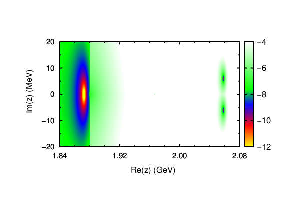
After inclusion of the coupled-channel effect, there are still two poles produced near two thresholds, and it is obvious that the higher and lower poles correspond to the and channels, respectively. As expected, the higher pole from the channel will deviated form the real axis after inclusion of the coupling of two channels as shown in Fig. 1, which reflects the decay width from opening the decay of the channel. The pole for the lower pole is still at real axis because no decay channel is open in the calculation.
In Table 4, the poles from the interaction with the variations of two cutoffs are presented. Empirically, the larger cutoff will lead to a larger coupling of two channels as well as the one-channel interaction. It is well reflected in the results listed in Table 4. When we fix and increase , both poles run farther away from the thresholds but from different origins. The upper pole, which is produced from the interaction, runs fast because the cutoff affects the strength of the interaction directly. The lower pole runs relatively slowly because the cutoff does not sffect the interaction, which produces this pole. The origin of running of the lower pole is the enhancement of the coupling of two channels. When we fix and increase , similar phenomena can be found.
| 0.8 | 1.0 | 1.2 | 1.4 | 1.6 | |
|---|---|---|---|---|---|
| 1.5 | 2086+ | 2081+2 | 2068+4 | 2046+8 | 1994+12 |
| 1880 | 1879 | 1879 | 1878 | 1878 | |
| 1.7 | 2086+ | 2081+2 | 2067+4 | 2046+8 | 1995+11 |
| 1874 | 1874 | 1873 | 1871 | 1869 | |
| 1.9 | 2086+ | 2081+3 | 2067+5 | 2046+8 | 1.995+10 |
| 1831 | 1828 | 1824 | 1819 | 1810 | |
| 2.1 | 2086+ | 2081+3 | 2067+5 | 2045+7 | 1993+8 |
The width of the higher pole increases with the increase of cutoff at all fixed values of cutoff , which is a mixing effect of the enhancement of the coupling of two channels and fast running of the higher pole. When the cutoff increases at fixed , the width decreases relatively slowly because the upper pole is produced from the interaction, which is independent of the cutoff . Also, at larger , the width becomes smaller with an increase of the cutoff . It is reasonable because the width of the pole will increase first and then decrease when the pole runs away from the threshold.
Generally speaking, after inclusion of the coupled-channel effect of the and channels, the conclusion obtained with the one-channel calculation is unchanged; that is, two bound states are produced from the and channels, respectively.
V SUMMARY
The previous studies suggested the in the photoproduction is a three-quark state in the constituent quark model [30, 35], which makes it difficult to put the and in the photoproduction into the constituent quark model. Such difficulty and the closeness of the and to the and thresholds invoke us to consider the possibility of interpreting this two nucleon resonances in the hadronic molecular state picture, which is analogous to the LHCb pentaquarks.
In the one-boson-exchange model, the interaction potentials are obtained with the effective Lagrangians with the coupling constants fixed by the SU(3) symmetry. The bound states from the interactions are studied through solving the quasipotential Bethe-Salpeter equation. A bound state with quantum number from the interaction and a bound state with from the interaction are produced with reasonable cutoffs. These two bound states can be related to the and the , respectively. The results for these two bound states are also stable with the variation of the cutoff. Other bound states are also produced from the two interactions. However, they leave the threshold rapidly with an increase of the cutoff. Hence, though these bound states can be produced in a narrow window of the cutoff, the possibility of their existence in the real world is very small. The coupled-channel effect from the coupling of the and channels is also discussed, and it is found that the conclusion with the one-channel calculation is unchanged after inclusion of the coupled-channel effect.
With such an assignment, three nucleon resonances, , in photoproduction, and in photoproduction with , can be well understood. The two hadronic molecular states, and , can be seen as the strange partners of the LHCb pentaquarks. The difference is that in the hidden-strangeness sector, the two states are both in an S wave while in the hidden-charm sector; we should put one state in a P wave to reproduce the spin-parity suggested by the LHCb experiment.
Acknowledgments
This project is partially supported by the National Natural Science Foundation of China (Grant No.11675228) , and the Major State Basic Research Development Program in China (Grant No. 2014CB845405).
References
- [1] T. Nakano et al. [LEPS Collaboration], “Evidence for a narrow S = +1 baryon resonance in photoproduction from the neutron,” Phys. Rev. Lett. 91, 012002 (2003)
- [2] F. Close, “Vanishing pentaquarks,” Nature 435, 287 (2005).
- [3] R. Aaij et al. [LHCb Collaboration], “Observation of Resonances Consistent with Pentaquark States in Decays,” Phys. Rev. Lett. 115, 072001 (2015)
- [4] L. Roca, J. Nieves and E. Oset, “LHCb pentaquark as a molecular state,” Phys. Rev. D 92, no. 9, 094003 (2015)
- [5] J. He, “ and interactions and the LHCb hidden-charmed pentaquarks,” Phys. Lett. B 753, 547 (2016)
- [6] J. He, “Understanding spin parities of and in hadronic molecular state picture,” Phys. Rev. D. 95, 074004 (2017)
- [7] R. Chen, X. Liu, X. Q. Li and S. L. Zhu, “Identifying exotic hidden-charm pentaquarks,” Phys. Rev. Lett. 115, no. 13, 132002 (2015)
- [8] Z. C. Yang, Z. F. Sun, J. He, X. Liu and S. L. Zhu, “The possible hidden-charm molecular baryons composed of anti-charmed meson and charmed baryon,” Chin. Phys. C 36, 6 (2012)
- [9] L. Maiani, A. D. Polosa and V. Riquer, “The New Pentaquarks in the Diquark Model,” Phys. Lett. B 749, 289 (2015)
- [10] X. H. Liu, Q. Wang and Q. Zhao, “Understanding the newly observed heavy pentaquark candidates,” Phys. Lett. B 757, 231 (2016)
- [11] H. X. Chen, W. Chen, X. Liu, T. G. Steele and S. L. Zhu, “Towards exotic hidden-charm pentaquarks in QCD,” Phys. Rev. Lett. 115, no. 17, 172001 (2015)
- [12] U. G. Meissner and J. A. Oller, “Testing the composite nature of the ,” Phys. Lett. B 751, 59 (2015)
- [13] R. F. Lebed, “The Pentaquark Candidates in the Dynamical Diquark Picture,” Phys. Lett. B 749, 454 (2015)
- [14] R. Chen, J. He and X. Liu, “Possible strange hidden-charm pentaquarks from and interactions,” arXiv:1609.03235 [hep-ph].
- [15] S. G. Yuan, K. W. Wei, J. He, H. S. Xu and B. S. Zou, “Study of five quark system with three kinds of quark-quark hyperfine interaction,” Eur. Phys. J. A 48, 61 (2012)
- [16] J. J. Wu, R. Molina, E. Oset and B. S. Zou, “Prediction of narrow and resonances with hidden charm above 4 GeV,” Phys. Rev. Lett. 105, 232001 (2010)
- [17] B. S. Zou and D. O. Riska, “The s anti-s component of the proton and the strangeness magnetic moment,” Phys. Rev. Lett. 95, 072001 (2005)
- [18] R. H. Dalitz and S. F. Tuan, “The phenomenological description of -K -nucleon reaction processes,” Annals Phys. 10, 307 (1960).
- [19] J. A. Oller and U. G. Meissner, “Chiral dynamics in the presence of bound states: Kaon nucleon interactions revisited,” Phys. Lett. B 500, 263 (2001)
- [20] N. Kaiser, P. B. Siegel and W. Weise, “Chiral dynamics and the low-energy kaon - nucleon interaction,” Nucl. Phys. A 594, 325 (1995)
- [21] E. Oset and A. Ramos, “Nonperturbative chiral approach to s wave anti-K N interactions,” Nucl. Phys. A 635, 99 (1998)
- [22] D. Jido, T. Sekihara, Y. Ikeda, T. Hyodo, Y. Kanada-En’yo and E. Oset, “The nature of Lambda(1405) hyperon resonance in chiral dynamics,” Nucl. Phys. A 835, 59 (2010)
- [23] J. M. M. Hall, W. Kamleh, D. B. Leinweber, B. J. Menadue, B. J. Owen, A. W. Thomas and R. D. Young, “Lattice QCD Evidence that the Λ(1405) Resonance is an Antikaon-Nucleon Molecule,” Phys. Rev. Lett. 114, no. 13, 132002 (2015)
- [24] B. Krippa, “Chiral dynamics of the low-energy kaon - baryon interactions,” Phys. Rev. C 58, 1333 (1998)
- [25] M. Mai and U. G. Meißner, “Constraints on the chiral unitary amplitude from photoproduction data,” Eur. Phys. J. A 51, no. 3, 30 (2015)
- [26] M. Mai, P. C. Bruns and U. G. Meissner, “Pion photoproduction off the proton in a gauge-invariant chiral unitary framework,” Phys. Rev. D 86, 094033 (2012)
- [27] T. Inoue, E. Oset and M. J. Vicente Vacas, “Chiral unitary approach to S wave meson baryon scattering in the strangeness S = 0 sector,” Phys. Rev. C 65, 035204 (2002)
- [28] K. A. Olive et al. [Particle Data Group Collaboration], “Review of Particle Physics,” Chin. Phys. C 38, 090001 (2014).
- [29] A. V. Anisovich, R. Beck, E. Klempt, V. A. Nikonov, A. V. Sarantsev and U. Thoma, “Properties of baryon resonances from a multichannel partial wave analysis,” Eur. Phys. J. A 48, 15 (2012)
- [30] J. He and X. R. Chen, “The roles of nucleon resonances in (1520) photoproduciton off proton,” Phys. Rev. C 86, 035204 (2012)
- [31] J. He, “Internal structures of the nucleon resonances N(1875) and N(2120),” Phys. Rev. C 91, no. 1, 018201 (2015)
- [32] H. Kohri et al. [LEPS Collaboration], “Near-threshold Lambda(1520) production by the vec-gamma p —¿ K+ Lambda(1520) reaction at forward K+ angles,” Phys. Rev. Lett. 104, 172001 (2010)
- [33] S. H. Kim, S. i. Nam, Y. Oh and H. C. Kim, “Contribution of higher nucleon resonances to photoproduction,” Phys. Rev. D 84, 114023 (2011)
- [34] J. J. Xie and J. Nieves, “The role of the resonance in the reaction,” Phys. Rev. C 82, 045205 (2010)
- [35] J. He, “Theoretical study of the Λ(1520) photoproduction off proton target based on the new CLAS data,” Nucl. Phys. A 927, 24 (2014)
- [36] K. Moriya et al. [CLAS Collaboration], “Differential Photoproduction Cross Sections of the , , and ,” Phys. Rev. C 88, 045201 (2013) Addendum: [Phys. Rev. C 88, no. 4, 049902 (2013)]
- [37] J. J. Xie, E. Wang and J. Nieves, “Re-analysis of the photoproduction reaction,” Phys. Rev. C 89, no. 1, 015203 (2014)
- [38] T. Mibe et al. [LEPS Collaboration], “Diffractive phi-meson photoproduction on proton near threshold,” Phys. Rev. Lett. 95, 182001 (2005)
- [39] A. Kiswandhi, J. J. Xie and S. N. Yang, “Is the nonmonotonic behavior in the cross section of phi photoproduction near threshold a signature of a resonance?,” Phys. Lett. B 691, 214 (2010)
- [40] A. Kiswandhi and S. N. Yang, “On the near-threshold peak structure in the differential cross section of -meson photoproduction: indication of a missing resonance with non-negligible strangeness content,” Phys. Rev. C 86, 015203 (2012) Erratum: [Phys. Rev. C 86, 019904 (2012)]
- [41] W. C. Chang et al. [LEPS Collaboration], “Measurement of Spin-Density Matrix Elements for -Meson Photoproduction from Protons and Deuterons Near Threshold,” Phys. Rev. C 82, 015205 (2010)
- [42] W. C. Chang et al. [LEPS Collaboration], “Measurement of the incoherent photoproduction near threshold,” Phys. Lett. B 684, 6 (2010)
- [43] X. Qian et al., “Near-threshold Photoproduction of Phi Mesons from Deuterium,” Phys. Lett. B 696, 338 (2011)
- [44] A. Kiswandhi, S. N. Yang and Y. B. Dong, “Near-threshold incoherent photoproduction on the deuteron: Searching for traces of a resonance,” Phys. Rev. C 94, no. 1, 015202 (2016)
- [45] H. Seraydaryan et al. [CLAS Collaboration], “-meson photoproduction on Hydrogen in the neutral decay mode,” Phys. Rev. C 89, no. 5, 055206 (2014)
- [46] R. F. Lebed, “Diquark substructure in ϕ photoproduction,” Phys. Rev. D 92, no. 11, 114006 (2015)
- [47] S. Sarkar, E. Oset and M. J. Vicente Vacas, “Baryonic resonances from baryon decuplet-meson octet interaction,” Nucl. Phys. A 750, 294 (2005) Erratum: [Nucl. Phys. A 780, 90 (2006)]
- [48] J. J. de Swart, “The Octet model and its Clebsch-Gordan coefficients,” Rev. Mod. Phys. 35, 916 (1963) Erratum: [Rev. Mod. Phys. 37, 326 (1965)].
- [49] G. Janssen, K. Holinde and J. Speth, “pi rho correlations in the N N potential,” Phys. Rev. C 54, 2218 (1996).
- [50] D. Ronchen et al., “Coupled-channel dynamics in the reactions ,” Eur. Phys. J. A 49, 44 (2013)
- [51] A. Matsuyama, T. Sato and T.-S. H. Lee, “Dynamical coupled-channel model of meson production reactions in the nucleon resonance region,” Phys. Rept. 439, 193 (2007)
- [52] P. Gao, B. S. Zou and A. Sibirtsev, “Analysis of the new Crystal Ball data on reaction with beam momenta of MeV/,” Nucl. Phys. A 867, 41 (2011)
- [53] M. Bando, T. Kugo and K. Yamawaki, “Nonlinear Realization and Hidden Local Symmetries,” Phys. Rept. 164, 217 (1988).
- [54] G. Janssen, K. Holinde and J. Speth, “A Meson exchange model for pi rho scattering,” Phys. Rev. C 49, 2763 (1994).
- [55] F. Gross and A. Stadler, “Covariant spectator theory of np scattering: Phase shifts obtained from precision fits to data below 350-MeV,” Phys. Rev. C 78, 014005 (2008)
- [56] F. Gross and A. Stadler, “Covariant spectator theory of scattering: Effective range expansions and relativistic deuteron wave functions,” Phys. Rev. C 82, 034004 (2010)
- [57] J. He, “Study of the bound states in a Bethe-Salpeter approach,” Phys. Rev. D 90, no. 7, 076008 (2014)
- [58] J. He and P. L. Lü, “Understanding Y(4274) and X(4320) in the invariant mass spectrum,” Nucl. Phys. A 919, 1 (2013)
- [59] J. He, “The as a resonance from the interaction,” Phys. Rev. D 92, no. 3, 034004 (2015)
- [60] F. Gross, “Charge conjugation invariance of the spectator equations,” Few Body Syst. 30, 21 (2001)
- [61] J. He and P. L. Lü, “The octet meson and octet baryon interaction with strangeness and the ,” Int. J. Mod. Phys. E 24, no. 11, 1550088 (2015)
- [62] J. He and P. L. Lü, “ and interactions and the charged charmonium-like state ,” Chin. Phys. C 40, no. 4, 043101 (2016)
- [63] P. L. Lü and J. He, “Hadronic molecular states from the interaction,” Eur. Phys. J. A 52, no. 12, 359 (2016)
- [64] J. A. Oller, E. Oset and J. R. Pelaez, “Meson meson interaction in a nonperturbative chiral approach,” Phys. Rev. D 59, 074001 (1999) Erratum: [Phys. Rev. D 60, 099906 (1999)] Erratum: [Phys. Rev. D 75, 099903 (2007)]