Volkov States and Non-linear Compton Scattering in Short and Intense Laser Pulses
Abstract
The collision of ultra-relativistic electron beams with intense short laser pulses makes possible to study QED in the high-intensity regime. Present day high-intensity lasers mostly operate with short pulse durations of several tens of femtoseconds, i.e. only a few optical cycles. A profound theoretical understanding of short pulse effects is important not only for studying fundamental aspects of high-intensity laser matter interaction, but also for applications as novel X- and gamma-ray radiation sources. In this article we give a brief overview of the theory of high-intensity QED with focus on effects due to the short pulse duration. The non-linear spectral broadening in non-linear Compton scattering due to the short pulse duration and its compensation is discussed.
1 Introduction & High-Intensity Parameters
Rapid advances in tera- and petawatt-class laser technology allow to explore light-matter interactions in the experimentally uncharted high-intensity regime. Theoretical predictions include, for instance, intensity dependent non-linearities in high-energy photon emission and pair production processes [1], or non-linear quantum vacuum optics effects such as vacuum birefringence and photon splitting [2, 3, 4, 5]. Eventually one expects the spontaneous creation of particle anti-particle pairs from the vacuum (so-called Sauter-Schwinger effect) for field strengths on the order of11 1 We use natural Heaviside-Lorentz units with and fine structure constant . Scalar products between four-vectors are denoted as . [6, 7, 8, 9].
When an electron interacts with a high-intensity laser, the laser pulse can be described as a plane wave. Plane waves are null-fields, i.e. both field invariants vanish: , which means no pairs can be produced from vacuum via the Sauter-Schwinger mechanism). The majority of modern high-intensity laser systems produces laser pulses with wavelengths on the order of , and with pulse durations on the order of tens of femtoseconds, i.e. only a few optical cycles. We therefore shall investigate in this article the important effects of the short pulse duration in high-intensity laser matter interactions.
Let us first recall some of the properties of (transverse) plane waves, which we assume to propagate along the negative axis, and with frequency . Their wave vector is a light-like four-vector, , and the field strength is a univariate function, . In this case, , which tells us that the field depends solely on the light-front variable (cf. Appendix A). In addition, Maxwell’s equations in vacuum require that is transverse, . The field can be represented by a transverse vector potential, , with , and parametrized as with a complex polarization vector , and an envelope function with pulse duration . The interaction of a probe electron with four-momentum with the plane wave field can be characterized by the following dimensionless gauge and Lorentz invariant parameters: (i) the classical nonlinearity parameter [10], (ii) the quantum energy parameter , and (iii) the quantum efficiency parameter . For a pulsed laser field one has in addition the dephasing parameter [11], which represents the ratio of the laser peak intensity and the laser bandwidth .
The classical nonlinearity parameter represents the laser energy density seen by the probe electron and can be related to the laser intensity via . With present laser technology one is able to reach light intensities on the order of , which corresponds to at typical for Ti:Sa laser systems [12, 13]. With the upcoming generation of multi-petawatt lasers one expects to reach intensities up to and even beyond 22 2 For instance, the Vulcan laser at RAL-CLF (UK) ({http://www.clf.stfc.ac.uk/CLF/}), the ELI project (Czech Republic, Hungary, Romania) {http://www.eli-beams.eu}, or the OMEGA EP-OPAL project (Rochester, USA).. The parameter also represents the work done by the field in one wavelength of the wave in units of the electron mass . The limit , refers to both the limit of infinite intensity at fixed frequency and the static limit () at fixed intensity. For the probabilities of processes happening in the laser field approach those in a constant crossed field [1] and are described by the quantum efficiency parameter alone. The regime is also referred to as “quasi-static” or “tunnelling” regime, i.e. serves as the Keldysh parameter of the electron laser interaction.
The quantum efficiency parameter is the value of the electric field experienced by the particle in its rest frame in units of the Sauter-Schwinger field strength, , with . This means that can be large for ultra-relativistic particles with colliding with a laser pulse, although the electric field in the laboratory frame is much weaker than due to the Lorentz transformation of the transverse electric field.
2 Classical Dynamics of an Electron in a Laser Pulse
Before we dive into the quantum theory of the laser matter interaction let us start with a classical description. The classical picture is valid whenever both the quantum energy parameter and the quantum efficiency parameter . According to the classical theory of electrodynamics, the dynamics of point-like charged particles in a given external field configuration, described by the field strength tensor , is governed by the Lorentz force equation [14]
| (1) |
where is the electron mass and we have conveniently absorbed the electron charge into the background field vector potential . The electron’s four-velocity is the tangent vector to the particle’s world line , parametrized by proper time . Due to the anti-symmetry of the field strength tensor the four-acceleration is always orthogonal to the four-velocity, and the four-velocity is normalized as .
In general this is a non-linear differential equation as the field strength has to be taken along the world line of the particle to be solved for . The solution of (1) can be quite a difficult task. For instance, the motion of an electron in standing waves can show chaotic behaviour [15]. Luckily, the dynamics of an electron in a plane wave laser field is one of the few exactly solvable cases.
2.1 Solution of the Lorentz Force Equation in Plane Waves
The solution of the Lorenz force equation in a plane wave field becomes particularly simple when employing light-front coordinates (cf. Appendix A), as one can find a very simple relation between the laser phase and the particle’s proper time . By dotting the laser wave-vector into the equation of motion (1) we immediately find . That means is a constant of motion, i.e. the component of the electron’s four-velocity is conserved . From this we find that the relation between the laser phase , light-front time and proper time can be expressed as
| (2) |
That means one can replace the proper time derivative by a light-front time derivative in the equations of motion. Since the normalized laser vector potential has only transverse components, , the transverse components of the Lorentz force equation can be written as
which gives because of (2). Because the four-velocity is normalized, , the fourth component of the velocity can be obtained simply via
The particle world line is obtain by integrating the four-velocity again
| (3) |
For later use we here also define the kinetic four momentum of the electron as . The solution for the kinetic momentum can also be represented in a covariant way as
| (4) |
where is the initial value of the momentum, and with
has the form of a Lorentz transformation [16, 17]. In particular, the minus-component of the kinetic electron momentum can be written as
| (5) |
2.2 Radiation Back-Reaction
When the electron interacts with a high-intensity laser pulse the back-reaction of the emission of radiation on the electron motion, the so-called radiation reaction (RR), can become significant. The radiation power is given by the Larmor formula, . Whenever the emitted radiation energy becomes comparable to the electron’s initial energy , the equations of motion (1) have to be amended by a radiation force term :
| (6) |
In the radiation dominated regime, characterized by the parameter , the electron loses a large fraction of it’s kinetic energy in one cycle of the background laser field, and the RR force becomes comparable to the Lorentz force. This regime could be reached, for instance by colliding a 500 MeV electron beam with a laser pulse with , which corresponds to a peak intensity of .
Many different forms for the RR force have been suggested since the seminal works of Lorenz and Abraham more than a century ago [18, 19, 20, 21]. A particularly popular form of the RR force (which is often used in numerical simulations of laser-matter interaction at high intensity [22, 23, 24]) is the so-called Landau-Lifshitz force [25]. It reads
| (7) |
The equations of motion (6) with the LL radiation force (7) also possess closed form analytic solutions in the presence of plane wave backgrounds [26]. By dotting again the laser wave-vector into the equations of motion we find
which can be integrated to find a (non-linear) relation between the laser phase and proper time [cf. (2)] allowing to integrate (6) [26].
Finally, we note that the classical RR is a continuous process, in contrast to quantum RR which is stochastic. Quantum RR effects are important whenever already the emission of a single photon can alter the electron trajectory significantly due to the momentum recoil [27, 28, 29]. The transition from the classical to the quantum RR regime is characterized by and [27].
3 High-intensity QED in the Furry Picture
In high-intensity QED the laser field is usually described as a background field33 3 However, the development of avalanche type QED cascades at extreme intensities could cause a depletion of the laser, turning an initially strong field weak, and rendering the background field approximation invalid [30, 31, 32, 33]. See also A. M. Fedotov’s contribution in this volume.. This background field has to be treated to all orders, which can be achieved by going to the Furry interaction picture in which the background field is treated as part of the unperturbed system [34]. For this we need to know the solutions of the Dirac equation
| (8) |
in a given background describing the laser field. The solutions of (8) in a univariate null-field background are called Volkov wave functions [35]. We use here the Dirac slash notation to denote scalar products between four-vectors and the Dirac matrices .
3.1 Derivation of Volkov States
Let us now explicitly calculate the Volkov wave functions. Although the derivation can be found in textbooks (e.g. in [36]) will be present it here in some detail to work out why a null-field background is required in order to solve Eq. (8) and indicate possible extensions to more general backgrounds. In the first step on transforms (8) into a second order differential equation by multiplying with the adjoint Dirac operator from the left [36], yielding
| (9) |
with as the commutator of gamma matrices. The so-called Pauli interaction term describes the interaction of the half-integer electron spin with the background field. The general idea is to seek a solution of (9) in the form with a constant four-vector , and where is a () Dirac matrix depending only on the laser phase and denotes a Dirac bi-spinor.
When switching off the background field, the quantum numbers represent the four-momentum of a free particle. With the background field present, they represent the asymptotic electron momentum outside the laser pulse. Because three momentum operators , and commute with the Dirac-operator, the corresponding quantum numbers are conserved. In addition, is determined by the mass shell condition . Similarly, the Dirac bi-spinors are the the free Dirac spinors for (on-shell) momentum , fulfilling , and where is the spin quantum number. We choose here and in the following the normalization .
By plugging the above ansatz for the wave function into (9) one obtains an equation for the unknown matrix function . Because Eq. (9) is a second order differential equation, in general the equation for can be expected to be a second order as well. However, the coefficient of the second order term turns out to be . That means for a light-like univariate background field with wave vector the equation for is of first order. Note that this is not true for space-like () or time-like () wave vectors. The first case, for instance, corresponds to magnetic undulators or the wave propagation in a medium with refractive index . The latter case may refer to time dependent electric fields, or the propagation of waves in a medium with refractive index , e.g. a plasma. No general solutions of relativistic wave equations exist in background fields with . Recent attempts to find (approximate) solutions can be found in Refs. [37, 38, 39, 40]. The situation becomes even more complicated for bi-variate backgrounds, for instance for the electron dynamics in two counter-propagating laser beams [41].
For the Volkov problem, with , we eventually find the following first order ordinary differential equation for the hitherto unknown matrix function :
| (10) |
This equation can be easily integrated yielding
| (11) | ||||
| (12) |
where we used that is a nilpotent operator of grade 2, i.e. , which again holds because the background field has a light-like wave vector with and . The non-linear phase can be written as an integrals of the minus component of the classical kinetic four-momentum (5) by using that . Note that the Volkov wave functions (14) are normalized using a covariant light-front normalization,44 4 The scalar product between any two spinor wave functions is defined in a Lorentz invariant way as [42] , with being a hypersurface in Minkowski space and the infinitesimal normal vector thereupon. The hypersurface can be expressed in general curvilinear coordinates , where defines the hypersurface and parametrize , such that with the determinant of the metric tensor in the coordinates . Choosing a light-front surface yields (13).
| (13) |
and where stands for , i.e. .
It is also convenient to define the so-called Ritus matrices , such that the Volkov states can be written as
| (14) |
The Ritus matrices can decomposed as , where denotes the classical Hamilton-Jacobi action of a classical particle in the background field. That means Volkov wave function is an exact semiclassical wavefunction, i.e. while being an exact solution of the wave equation (8) the action does not contain quantum corrections (in powers of ). The matrix is the bi-spinorial representation of the Lorentz transformation that generates the classical orbits (4), and which is defined by
The Lorentz transformation transports the spinor along the classical trajectory [16, 17]. The Ritus matrices, analytically continued to off-shell momenta , have the following orthogonality and completeness properties:
The wave functions (14) represent the positive energy solutions of (8), i.e. they describe the propagation of electrons in a background field. In order to describe positrons as well (for instance to calculate the probabilities for pair production in a laser field) we need the negative energy solutions of (8). They can be obtained from (14) via the transformation , i.e. , where the notation for negative energy spinors is as usual [43, 44].
3.2 Properties of Volkov States
The properties of the Volkov states can be studied by investigating the Ritus matrix function as they contain all the information on the interaction with the laser field. Since the are matrices it is reasonable to study the different projections onto the basis elements of the Clifford algebra [45]. It turns out that only the scalar and anti-symmetric tensor projections yield non-zero results:
| (15) | ||||
| (16) |
where , and tr denotes the trace over the Dirac matrix indices.

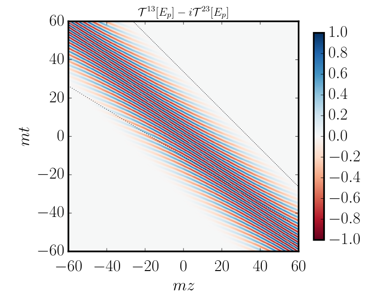
The real parts of the scalar projection and the combination of tensor projections are exhibited in Figure 1 for an electron with an energy of propagating head-on through a strong laser pulse with and a pulse duration . The two projections are shown in the frame where the electron is initially at rest. In that frame, the free electron wave function outside the laser pulse behaves as . In the case of the scalar projection of the Ritus matrices the effect of the laser pulse is a local tilt of the electron wave fronts, see left panel of Fig. 1. This behaviour corresponds to the build-up of an intensity dependent ponderomotive quasi-momentum inside the laser pulse [46]. The tensor projection of the Ritus matrices shown in the right panel of Fig. 1 are non-zero only in regions where the laser pulse is present. They correspond to the term in the Volkov states, i.e. the Pauli interaction term.
In the following we construct wave packets from the Volkov wave functions and show that the motion of the centroid of the packet follows is closely related to the classical trajectory [47, 48]. We will restrict the discussion to the scalar part of the Volkov wave function which describes charged spin-0 bosons. As a simple example it suffices to construct a one-dimensional wave packet as a superposition of Volkov waves with a light-front momentum distribution but all having the same transverse momenta ,
| (17) |
Such a wave packet has a finite temporal duration, but remains infinitely extended in the transverse coordinates. In the following we choose a Gaussian distribution with Gaussian width and with . The laser pulse parameters are the same as for Figures 1. This construction provides a localized wave packet in the (-) plane with a minimum Gaussian size at . This wavepacket is shown in Figure 2 in the (-) plane. The centroid of the wave packet follows the classical trajectory (black curve), which shows the close correspondence between the classical trajectory solutions and the Volkov wave functions. In addition, the Dirac-Volkov current
| (18) |
coincides with the classical four-velocity .

Let us now investigate the momentum space spectrum of the Volkov states and find relations to the classical motion. The Ritus matrices have a spectral representation as a superposition of plane waves
| (19) |
with the spectral components
| (20) |
which are be represented by the three scalar functions
| (21) |
The variable parametrizes the amount of light-front laser momentum which is exchanged between the electron and the background field. It can be interpreted as some continuous analogue to the number of exchanged laser photons.
Let us now investigate the limit of infinitely long monochromatic plane wave background fields (IPW), formally achieved by setting . In that case the background is a periodic function such that the Floquet theorem applies [49]: The solution of the Dirac equation (8) in a periodic background takes the form
| (22) |
where has the same periodicity as the background, and is called the quasi-momentum. The Fourier-zero mode, i.e. the non-periodic part of the non-linear phase in (12), has been absorbed into the definition of the quasi-momentum.
In the limit of an IPW background the momentum distribution functions (21) degenerate to a delta comb
| (23) |
with support at discrete momentum values . For arbitrary polarization of the background field the coefficients are related to generalized Bessel functions (see e.g. [50, 51]), and they turn into ordinary Bessel functions of the first kind in the case of circular polarization. The Volkov wave function in an IPW background appears as an infinite sum over discrete momentum states
| (24) |
which are also called Zel’dovich levels [52]. The level structure furnishes an easy interpretation of strong-field phenomena. For instance, the appearance of harmonics in the non-linear Compton spectra or the resonant singularities in second-order strong-field scattering processes can be seen as transitions between different Zel’dovich of the incident and final state Volkov electrons. Modifications of this level structure due to radiative corrections, i.e. the electron self-energy have been calculated as well [53].
If one now starts from the well known case of infinite monochromatic plane waves (with the discrete level structure) and looks at modifications due to finite pulse duration one finds a broadening of the Zel’dovich levels. There are two different contributions to the level broadening: (i) a bandwidth broadening due to the finite laser bandwidth (ii) a non-linear, intensity dependent broadening due to the gradual change in the laser intensity in a pulsed field. This second mechanism is related to the ponderomotive, i.e. slowly varying, part of the non-linear phase , and can be seen as a gradual build-up of an intensity-dependent quasi-momentum as the laser intensity increases [46]. Depending on the bandwidth and the peak intensity either of the two mechanisms can be dominating the broadening of the Zel’dovich levels. The broadened Zel’dovich levels are shown in Fig. 3.
The scalar spectral components of a Volkov state also have a close relation to the classical electron motion in a laser pulse. The effective range of values of is determined by the classical dynamics [51]. To be specific, the maximum and minimum values of the minus component of the kinetic four-momentum determine the cut-off values of via . Beyond those cut-off values the functions drop to zero exponentially fast. The reason is that only for the phase integrals in (21) posses real stationary phase points. Also the local minima and maxima of , which appear during the course of the laser pulse, lead to pronounced structures in the Volkov state spectral component . This is caused by a sudden change in the number of stationary phase points related to fold-type caustics. All the local extremal points of are indicated by red lines in Figure 1, connecting them to pronounced structures in the spectral components . One could possibly observe those spectral features of the Volkov states by using laser-assisted Compton scattering of X-rays [54].
3.3 The Dirac-Volkov Propagator
The laser-dressed Green’s function (Dirac-Volkov propagator) is the solution of an inhomogeneous Dirac equation in the background field with delta inhomogeneity, . Many different representations of this Dirac-Volkov propagator are known, see e.g. [55, 56, 57, 58, 59, 60, 1]. A particularly useful representation is given in terms of the Ritus matrix functions as [1]
| (25) |
where the free propagator in momentum space is given by . The Dirac-Volkov propagator is needed for the calculation of higher-order processes in laser fields such as nonlinear Double Compton scattering [61, 62, 63], laser assisted Bremsstrahlung [64] or laser assisted pair production in the field of a nucleus [65], as well as the calculation of radiative corrections such as the electron mass operator [66]. It is worth noting that the background field determines the pole structure of the propagator, with an infinite series of poles for infinite monochromatic plane waves and just a single pole plus finite resonances for short pulses [62, 67, 68, 69].
3.4 Strong-Field Feynman Rules
In order to calculate the S matrix elements of high-intensity QED processes one may employ the Feynman diagram technique in coordinate space. The Feynman rules for high-intensity QED in the Furry picture can be summarized as follows [60]:
- 1.
External incoming or outgoing electrons with momentum are represented by laser dressed Volkov wave function or , respectively. For incoming and outgoing positrons one uses the corresponding negative energy Volkov wave function and .
- 2.
An internal fermion line corresponds to the Dirac-Volkov propagator .
- 3.
Internal and external photon lines are translated into the free photon propagator and the free photon wave functions, respectively, see e.g. Ref. [45].
- 4.
Each interaction vertex corresponds to a factor and an integral over .
- 5.
Symmetry factors for identical particles etc. are the same as in usual QED.
| ††feynman-diagram: (Feynman diagram, (x7) |
Let us look at few examples. Firstly, the S matrix for non-linear Compton scattering, i.e. the emission of a high-energy photon by an electron moving in an intense laser field, given in Fig. 5 (a). This diagram is are forbidden in ordinary QED without the background field because it is impossible to fulfil four-momentum conservation. The background field provides the missing four-momentum to make this process possible. Diagram (a) translates into the formula
| (26) |
where the wave function of the emitted photon with momentum and polarization vector is given by . The non-linear Compton scattering is discussed in some more detail in Section 4.
The second example is the non-linear Double Compton scattering in (b), where two photons are emitted coherently by the same electron. Because the two emitted photons are indistinguishable the S matrix is represented by two diagrams with the outgoing photon lines interchanged. The S matrix for this process reads
The pole structure of the Dirac-Volkov propagator strongly affects the spectrum of the emitted photons [70, 61, 62].
4 Non-linear Compton Scattering
The process of non-linear Compton scattering in high-intensity lasers has been investigated theoretically since the early 1960’s [71, 72, 73, 74], but in most studies infinite monochromatic plane wave laser fields or constant crossed fields have been assumed. But as mentioned above, modern laser systems produce very short high-intensity pulses with only a few cycles oscillations of the laser’s electric field. The influence of the short laser pulse duration on the non-linear Compton process has been investigated in the recent years, see for instance Refs. [46, 75, 76, 77, 78, 79, 80, 81]. We shall here discuss some of the short pulse effects on the non-linear Compton spectra. Similar effects can be seen also for other processes occuring in strong and short laser pulses, for instance in the non-linear Breit-Wheeler pair production [43, 82, 83, 84, 85, 86].

The differential photon emission probability is given by , with the S matrix element from (26), and where the Lorentz invariant phase space of the final particles is conveniently parametrized by yielding
| (27) |
where refers to the average and summation over all initial and final particle polarization states, respectively. In the exponent of the amplitude we rediscover the classical kinetic momentum , which is now projected onto the four-momentum of the emitted photon.
When the probability (27) is analysed for an infinite monochromatic plane wave one finds a discrete spectrum of emitted harmonics, which can be understood in terms of quasi-momentum conservation . The emitted photons are dominantly emitted into a narrow cone with opening angle for and for , and with harmonic frequencies . For on the order of harmonics contribute to the spectrum. In non-linear Compton scattering with a short laser pulse one observes a broadening of the spectral lines (see Fig. 6), similar to the broadening to the Zel’dovich level structure of the Volkov states discussed in Section 3. First of all, in a short laser pulse the harmonics acquire a bandwidth due to the bandwidth of the laser. But there is also a intensity dependent ponderomotive broadening effect related to the gradual build-up of quasi-momentum as the electron enters the laser pulse. The ponderomotively broadened spectral lines have a (relative) bandwidth . One sees in Fig. 6 that the broadened spectral lines consist of a large number of subsidiary peaks. This can be explained as the interference of radiation emitted at the leading and trailing slopes of the pulse envelope [80]. It turns out that this ponderomotive broadening effect always occurs whenever the dephasing parameter . This is true also for quite weak laser pulses as long as the spectral bandwidth of the laser is sufficiently small [11].
This broadening effect, while being an interesting phenomenon in the interplay between bandwidth and intensity effects will be a severe limitation for the spectral brightness of inverse Compton backscattering x- and gamma-ray sources. One way of dealing with the broadening is to limit the laser intensity to an acceptable level of broadening for a specific application [87], which limits the brightness of the source, of course. A more advanced possibility is to use chirped laser pulses, i.e. with a time-dependent frequency. It has been shown theoretically that with properly chirped laser pulses (which are spectrally blue-shifted at the pulse centre where the intensity is highest) the spectral broadening can be compensated [88, 89, 79, 90], see Fig. 7. This opens an avenue towards bright narrowband hard-gamma radiation sources operated at large laser intensities .
5 Summary
In this article an overview of the theory of high-intensity QED was given with focus on effects due to the short pulse duration. Both the solutions of the classical equations of motion, as well as the Volkov wave functions and the Dirac-Volkov propagator in the case of high-field QED were presented. The spectrum of non-linear Compton scattering in short intense pulses was discussed. The intensity dependent spectral broadening can be compensated by chirping the laser pulse.
Appendix A: Light-Front Coordinates
Because the laser’s wave-vector (four-momentum vector) is a light like vector with it is very convenient to use so-called light-front co-ordinates to describe the dynamics of charged particles in laser background fields. Let us assume that the laser pulse propagates along the negative -axis, , such that it’s phase argument . That means the background field depends only on the single light-front variable . All particles will enter (leave) the laser pulse at the same value of the the light-front time coordinate , see Fig. 8.
The light-front components of a generic four-vector with Cartesian coordinates are defined as
| (28) |
The inverse coordinate transformation is given by and . We immediately find that the laser four-momentum has only a single non-vanishing component in light-front coordinates: The metric tensor in light-front coordinates, using the arrangement of components , has non-diagonal components
The covariant components of a four-vector are related to the contravariant components as
and scalar products between two four-vectors read
The Lorentz invariant integration measure in light-front coordinates is given by
with as the determinant of the metric tensor. For a four-dimensional delta distribution one writes in light-front form
where we introduced the short-hand notation . The free particle dispersion relations (mass shell conditions) read in light-front coordinates
for massive and massless particles, respectively. The Lorentz invariant on-shell phase space element is
with . Thus the Lorentz invariant on-shell delta distributions are given by .
The light-front components of the Dirac matrices obey the anti-commutation relations with the metric tensor (Appendix A: Light-Front Coordinates). In particular it follows that .
References
- [1] V. I. Ritus, “Quantum effects of the interaction of elementary particles with an intense electromagnetic field,” J. Sov. Laser Res. 6, 497 (1985).
- [2] G. V. Dunne, “The Heisenberg–Euler Effective Action: 75 Years On,” Int. J. Mod. Phys. A 27, 1260004 (2012).
- [3] T. Heinzl, B. Liesfeld, K.-U. Amthor, H. Schwoerer, R. Sauerbrey, and A. Wipf, “On the observation of vacuum birefringence,” Opt. Commun. 267, 318 (2006).
- [4] F. Karbstein and R. Shaisultanov, “Stimulated photon emission from the vacuum,” Phys. Rev. D 91, 113002 (2015).
- [5] H. Gies, F. Karbstein, and N. Seegert, “Photon merging and splitting in electromagnetic field inhomogeneities,” Phys. Rev. D 93, 085034 (2016).
- [6] J. Schwinger, “On Gauge Invariance and Vacuum Polarization,” Phys. Rev. 82, 664 (1951).
- [7] V. S. Popov, “On Schwinger mechanism of pair production from vacuum by the field of optical and X-ray lasers,” Phys. Lett. A 298, 83 (2002).
- [8] D. B. Blaschke, A. V. Prozorkevich, C. D. Roberts, S. M. Schmidt, and S. A. Smolyansky, “Pair production and optical lasers,” Phys. Rev. Lett. 96, 140402 (2006).
- [9] F. Hebenstreit, R. Alkofer, and H. Gies, “Pair production beyond the Schwinger formula in time-dependent electric fields,” Phys. Rev. D 78, 61701 (2008).
- [10] T. Heinzl and A. Ilderton, “A Lorentz and gauge invariant measure of laser intensity,” Opt. Commun. 282, 1879 (2009).
- [11] F. V. Hartemann, F. Albert, C. W. Siders, and C. P. J. Barty, “Low-Intensity Nonlinear Spectral Effects in Compton Scattering,” Phys. Rev. Lett. 105, 130801 (2010).
- [12] C. Danson, D. Hillier, N. Hopps, and D. Neely, “Petawatt class lasers worldwide,” High Power Laser Sci. Eng. 3, 1 (2015).
- [13] V. Yanovsky, V. Chvykov, G. Kalinchenko, P. Rousseau, T. Planchon, T. Matsuoka, A. Maksimchuk, J. Nees, G. Cheriaux, G. Mourou, et al., “Ultra-high intensity- 300-TW laser at 0.1 Hz repetition rate,” Opt. Express 16, 2109 (2008).
- [14] J. D. Jackson, Klassische Elektrodynamik, Walter de Gruyter, Berlin, New York, 2nd edition (1983).
- [15] D. Bauer, P. Mulser, and W. Steeb, “Relativistic ponderomotive force, Uphill acceleration, and transition to chaos.” Phys. Rev. Lett. 75, 4622 (1995).
- [16] R. W. Brown and K. L. Kowalski, “Volkov Solutions, Gauge-Poincaré Transformations, and Plane-Wave Decoupling,” Phys. Rev. Lett. 51, 2355 (1983).
- [17] R. W. Brown and K. L. Kowalski, “Gauge couplings as local gauge and Poincaré transformations: Generalized Taub-Volkov solutions,” Phys. Rev. D 30, 2602 (1984).
- [18] M. Abraham, “Prinzipien der Dynamik des Elektrons,” Ann. Phys. 315, 105 (1902).
- [19] P. Dirac, “Classical theory of radiating electrons,” Proc. R. Soc. Lond. Ser. A 167, 148 (1938).
- [20] I. V. Sokolov, N. M. Naumova, J. A. Nees, G. A. Mourou, and V. P. Yanovsky, “Dynamics of emitting electrons in strong laser fields,” Phys. Plasmas 16 (2009).
- [21] A. Ilderton and G. Torgrimsson, “Radiation reaction in strong field QED,” Phys. Lett. B 725, 481 (2013).
- [22] R. Capdessus, E. D’Humières, and V. T. Tikhonchuk, “Modeling of radiation losses in ultrahigh power laser-matter interaction.” Phys. Rev. E 86, 036401 (2012).
- [23] M. Vranic, J. Martins, R. Fonseca, and L. Silva, “Classical radiation reaction in particle-in-cell simulations,” Comput. Phys. Commun. 204, 141 (2016), 1502.02432.
- [24] S. Tang, N. Kumar, and C. H. Keitel, “Optimized plasma high harmonics generation from ultra-intense laser pulses,” arXiv:1608.02513 (2016).
- [25] L. D. Landau and E. M. Lifschitz, Klassische Feldtheorie, volume 2 of Lehrbuch der Theoretischen Physik, Akademie Verlag, 12th editi edition (1992).
- [26] A. Di Piazza, “Exact solution of the Landau-Lifshitz equation in a plane wave,” Lett. Math. Phys. 83, 305 (2008).
- [27] A. Di Piazza, K. Z. Hatsagortsyan, and C. H. Keitel, “Quantum Radiation Reaction Effects in Multiphoton Compton Scattering,” Phys. Rev. Lett. 105, 220403 (2010).
- [28] N. Neitz and A. Di Piazza, “Stochasticity Effects in Quantum Radiation Reaction,” Phys. Rev. Lett. 111, 054802 (2013).
- [29] T. G. Blackburn, C. P. Ridgers, J. G. Kirk, and A. R. Bell, “Quantum Radiation Reaction in Laser–Electron-Beam Collisions,” Phys. Rev. Lett. 112, 015001 (2014).
- [30] A. M. Fedotov, N. B. Narozhny, G. Mourou, and G. Korn, “Limitations on the Attainable Intensity of High Power Lasers,” Phys. Rev. Lett. 105, 080402 (2010).
- [31] S. S. Bulanov, T. Z. Esirkepov, A. G. R. Thomas, J. K. Koga, and S. V. Bulanov, “Schwinger Limit Attainability with Extreme Power Lasers,” Phys. Rev. Lett. 105, 220407 (2010).
- [32] P. Zhang, C. P. Ridgers, and A. G. R. Thomas, “The effect of nonlinear quantum electrodynamics on relativistic transparency and laser absorption in ultra-relativistic plasmas,” New J. Phys. 17, 043051 (2015), arXiv:1403.5034.
- [33] D. Seipt, T. Heinzl, M. Marklund, and S. S. Bulanov, “Depletion of intense fields,” arXiv:1605.00633 (2016).
- [34] W. H. Furry, “On Bound States and Scattering in Positron Theory,” Phys. Rev. 81, 115 (1951).
- [35] D. M. Volkov, “Über eine Klasse von Lösungen der Diracschen Gleichung,” Z. Phys. 94, 250 (1935).
- [36] W. B. Berestetzki, E. M. Lifschitz, and L. P. Pitajewski, Relativistische Quantentheorie, volume IV of Lehrbuch der Theoretischen Physik, Akademie Verlag, Berlin (1980).
- [37] T. Heinzl, A. Ilderton, and B. King, “Classical and quantum particle dynamics in univariate background fields,” Phys. Rev. D 94, 065039 (2016).
- [38] E. Raicher and S. Eliezer, “Analytical solutions of the Dirac and the Klein-Gordon equations in plasma induced by high-intensity laser,” Phys. Rev. A 88, 022113 (2013).
- [39] E. Raicher, S. Eliezer, and A. Zigler, “A novel solution to the Klein–Gordon equation in the presence of a strong rotating electric field,” Phys. Lett. B 750, 76 (2015), 1502.03558.
- [40] J. T. Mendonça and A. Serbeto, “Volkov solutions for relativistic quantum plasmas,” Phys. Rev. E 83, 026406 (2011).
- [41] B. King and H. Hu, “Classical and quantum dynamics of a charged scalar particle in a background of two counterpropagating plane waves,” arXiv:1609.08105 (2016).
- [42] V. G. Bagrov and D. M. Gitman, Exact Solutions of Relativistic Wave Equations, Kluwer Academic Publishers, Dordrecht (1990).
- [43] T. Nousch, D. Seipt, B. Kämpfer, and A. Titov, “Pair production in short laser pulses near threshold,” Phys. Lett. Sect. B Nucl. Elem. Part. High-Energy Phys. 715, 246 (2012).
- [44] C. Itzykson and J.-B. Zuber, Quantum Field Theory, McGraw-Hill (1980).
- [45] M. E. Peskin and D. V. Schroeder, An Introduction to Quantum Field Theory, Addison-Wesley Publishing Company (1995).
- [46] N. B. Narozhnyi and M. S. Fofanov, “Photon emission by an electron in a collision with a short focused laser pulse,” J. Exp. Theor. Phys. 83, 14 (1996).
- [47] R. A. Neville and F. Rohrlich, “Quantum Electrodynamics on Null Planes and Applications to Lasers,” Phys. Rev. D 3, 1692 (1971).
- [48] S. Zakowicz, “Square-integrable wave packets from the Volkov solutions,” J. Math. Phys. 46, 032304 (2005).
- [49] G. Floquet, “Sur les équations différentielles linéaires à coefficients périodiques,” Ann. l’École Norm. Supérieure 12, 47 (1883).
- [50] H. J. Korsch, A. Klumpp, and D. Witthaut, “On two-dimensional Bessel functions,” J. Phys. A 39, 14947 (2006).
- [51] E. Loetstedt and U. D. Jentschura, “Recursive algorithm for arrays of generalized Bessel functions: Numerical access to Dirac-Volkov solutions,” Phys. Rev. E 79, 026707 (2009).
- [52] Y. B. Zel’dovich, “The Quasienergy of a Quantum-Mechanical System Subjected to a Periodic Action,” Sov. Phys. J. Exp. Theor. Phys. 24, 1006 (1967).
- [53] W. Becker and H. Mitter, “Modification of the quasi-levels of an electron in a laser field due to radiative corrections,” J. Phys. A 9, 2171 (1976).
- [54] D. Seipt, A. Surzhykov, S. Fritzsche, and B. Kämpfer, “Caustic structures in x-ray Compton scattering off electrons driven by a short intense laser pulse,” New J. Phys. 18, 023044 (2016).
- [55] J. H. Eberly and H. R. Reiss, “Electron Self-Energy in Intense Plane-Wave Field,” Phys. Rev. 145, 1035 (1966).
- [56] L. S. Brown and T. W. B. Kibble, “Interaction of intense laser beams with electrons,” Phys. Rev. 133, A705 (1964).
- [57] T. W. B. Kibble, A. Salam, and J. Strathdee, “Intensity-dependent mass shift and symmetry breaking,” Nucl. Phys. B 96, 255 (1975).
- [58] V. N. Baĭer, V. M. Katkov, and V. M. Strakhovenko, “Operator approach to quantum electrodynamics in an external field. Electron loops,” Sov. Phys. J. Exp. Theor. Phys. 41, 198 (1975).
- [59] V. N. Baĭer, A. I. Mil’shteĭn, and V. M. Strakhovenko, “Interaction between a photon and an intense electromagnetic wave,” Sov. Phys. J. Exp. Theor. Phys. 42, 961 (1976).
- [60] H. Mitter, “Quantum Electrodynamics in Laser Fields,” Acta Phys. Austriaca, Suppl. XIV pages 397–468 (1975).
- [61] E. Lötstedt and U. D. Jentschura, “Nonperturbative Treatment of Double Compton Backscattering in Intense Laser Fields,” Phys. Rev. Lett. 103, 110404 (2009).
- [62] D. Seipt and B. Kämpfer, “Two-photon Compton process in pulsed intense laser fields,” Phys. Rev. D 85, 101701 (2012).
- [63] F. Mackenroth and A. Di Piazza, “Nonlinear double Compton scattering in the full quantum regime,” Phys. Rev. Lett. 110, 070402 (2013).
- [64] E. Lötstedt, U. D. Jentschura, and C. H. Keitel, “Evaluation of Laser-Assisted Bremsstrahlung with Dirac-Volkov Propagators,” Phys. Rev. Lett. 98, 043002 (2007).
- [65] E. Lötstedt, U. D. Jentschura, and C. H. Keitel, “Laser Channeling of Bethe-Heitler Pairs,” Phys. Rev. Lett. 101, 203001 (2008).
- [66] V. Ritus, “Radiative corrections in quantum electrodynamics with intense field and their analytical properties,” Ann. Phys. (N. Y). 69, 555 (1972).
- [67] D. Seipt, Strong Field QED Processes in Short Laser Pulses, Ph.D. thesis, Technische Universität Dresden (2012).
- [68] A. Ilderton and G. Torgrimsson, “Scattering in plane-wave backgrounds: Infrared effects and pole structure,” Phys. Rev. D 87, 085040 (2013).
- [69] M. Lavelle, D. McMullan, and M. Raddadi, “Propagation in an intense background,” Phys. Rev. D 87, 085024 (2013), 1301.3072.
- [70] V. P. Oleĭnik, “Resonance effects in the field of an intense laser beam,” Sov. Phys. J. Exp. Theor. Phys. 25, 697 (1967).
- [71] A. I. Nikishov and V. I. Ritus, “Quantum processes in the field of a plane electromagnetic wave and in a constant field. I,” Sov. Phys. J. Exp. Theor. Phys. 19, 529 (1964).
- [72] A. I. Nikishov and V. I. Ritus, “Quantum processes in the field of a plane electromagnetic wave and in a constant field,” Sov. Phys. J. Exp. Theor. Phys. 19, 1191 (1964).
- [73] A. I. Nikishov and V. I. Ritus, “Nonlinear effects in Compton scattering and pair production owing to absorption of several photons,” Sov. Phys. J. Exp. Theor. Phys. 20, 757 (1965).
- [74] N. B. Narozhnyi, A. I. Nikishov, and V. I. Ritus, “Quantum processes in the field of a circularly polarized electromagnetic wave,” Sov. Phys. J. Exp. Theor. Phys. 20, 622 (1965).
- [75] M. Boca and V. Florescu, “Nonlinear Compton scattering with a laser pulse,” Phys. Rev. A 80, 053403 (2009).
- [76] D. Seipt and B. Kämpfer, “Non-Linear Compton Scattering of Ultrashort and Intense Laser Pulses,” Phys. Rev. A 83, 022101 (2011).
- [77] F. Mackenroth and A. Di Piazza, “Nonlinear Compton scattering in ultra-short laser pulses,” Phys. Rev. A 83, 032106 (2011).
- [78] K. Krajewska and J. Z. Kamiński, “Compton Process in Intense Short Laser Pulses,” Phys. Rev. A 85, 062102 (2012).
- [79] D. Seipt, S. G. Rykovanov, A. Surzhykov, and S. Fritzsche, “Narrowband inverse Compton scattering x-ray sources at high laser intensities,” Phys. Rev. A 91, 033402 (2015).
- [80] V. Y. Kharin, D. Seipt, and S. G. Rykovanov, “Temporal laser-pulse-shape effects in nonlinear Thomson scattering,” Phys. Rev. A 93, 063801 (2016), 1602.03062.
- [81] D. Seipt, V. Kharin, S. Rykovanov, A. Surzhykov, and S. Fritzsche, “Analytical results for nonlinear Compton scattering in short intense laser pulses,” J. Plasma Phys. 82, 655820203 (2016).
- [82] K. Krajewska and J. Z. Kamiński, “Breit-Wheeler process in intense short laser pulses,” Phys. Rev. A 86, 052104 (2012).
- [83] A. I. Titov, H. Takabe, B. Kämpfer, and A. Hosaka, “Enhanced Subthreshold Production in Short Laser Pulses,” Phys. Rev. Lett. 108, 240406 (2012).
- [84] A. I. Titov, B. Kämpfer, A. Hosaka, T. Nousch, and D. Seipt, “Determination of the carrier envelope phase for short, circularly polarized laser pulses,” Phys. Rev. D 93, 045010 (2016).
- [85] S. Meuren, C. H. Keitel, and A. Di Piazza, “Semiclassical picture for electron-positron photoproduction in strong laser fields,” Phys. Rev. D 93, 085028 (2016).
- [86] M. J. A. Jansen, J. Z. Kamiński, K. Krajewska, and C. Müller, “Strong-field Breit-Wheeler pair production in short laser pulses: Relevance of spin effects,” Phys. Rev. D 94, 013010 (2016).
- [87] F. V. Hartemann and S. S. Q. Wu, “Nonlinear Brightness Optimization in Compton Scattering,” Phys. Rev. Lett. 111, 044801 (2013).
- [88] I. Ghebregziabher, B. A. Shadwick, and D. Umstadter, “Spectral Bandwidth Reduction of Thomson Scattered Light by Pulse Chirping,” Phys. Rev. ST Accel. Beams 16, 030705 (2013).
- [89] B. Terzić, K. Deitrick, A. S. Hofler, and G. A. Krafft, “Narrow-Band Emission in Thomson Sources Operating in the High-Field Regime,” Phys. Rev. Lett. 112, 074801 (2014).
- [90] S. G. Rykovanov, C. G. R. Geddes, C. B. Schroeder, E. Esarey, and W. P. Leemans, “Controlling the spectral shape of nonlinear Thomson scattering with proper laser chirping,” Phys. Rev. Accel. Beams 19, 030701 (2016).