Simplified derivation of the collision probability of two objects in independent Keplerian orbits
Abstract
Many topics in planetary studies demand an estimate of the collision probability of two objects moving on nearly Keplerian orbits. In the classic works of Öpik [12] and Wetherill [17], the collision probability was derived by linearizing the motion near the collision points, and there is now a vast literature using their method. We present here a simpler and more physically motivated derivation for non-tangential collisions in Keplerian orbits, as well as for tangential collisions that were not previously considered. Our formulas have the added advantage of being manifestly symmetric in the parameters of the two colliding bodies. In common with the Öpik-Wetherill treatments, we linearize the motion of the bodies in the vicinity of the point of orbit intersection (or near the points of minimum distance between the two orbits) and assume a uniform distribution of impact parameter within the collision radius. We point out that the linear approximation leads to singular results for the case of tangential encounters. We regularize this singularity by use of a parabolic approximation of the motion in the vicinity of a tangential encounter.
I Introduction
An accurate estimate of the intrinsic collision probability between two objects moving on independent Keplerian orbits is essential in many topics in planetary system studies: the impact flux of interplanetary dust particles and minor planets on the Earth and other planets [12, 11, 8], evolution of the orbits of a swarm of planetesimals [4], planet formation [18], dynamical lifetimes of small bodies [3], collisional evolution of asteroids [1], the impact hazard of near-Earth asteroids [7], and collisions amongst artificial Earth-orbiting satellites [10].
In such problems, one usually wishes to quantify the probability of collision within some volume of space which is small compared to the uncertainties of the orbital parameters of the objects that pass through that volume; the objects are assumed to be moving on independent Keplerian orbits about a central body. Öpik [12] derived an equation for this collision probability for the case when one of the objects is assumed to be in a circular orbit. Wetherill [17] generalized this solution to two eccentric orbits. Öpik’s and Wetherill’s approaches have two steps in the calculation of collision probability. First, the collision probability for two intersecting Keplerian orbits is calculated. We call this probability , which is a function of the collision radius and the orbital elements defining the shape and the orientation of the two orbits. The two orbits are assumed to be fixed in space, and the mean anomalies are assumed to be independent (i.e., there is no mean motion resonance between the two bodies). Then, over a long period of time, the pair of objects has a well-defined probability of impact near the location where the two orbits intersect or where the distance between the two orbits is small enough for collision to be possible. (The collision radius is inflated from the sum of the physical radii of the bodies, to account for the gravitational focusing effect from their mutual interaction.) Secondly, for ensembles of bodies, the equation for works as a back-bone to calculate the average collision probability marginalized over all values of the mutual argument of pericenter, . For most values of , the minimum distance between two orbits is much larger than the distance that allows collision. Thus, the specific ranges of that allow the collision condition is calculated and over those intervals is integrated over the entire range.
In most previous works in the context of collision rates of asteroids, it has been assumed that apsidal and nodal precession rates are uniform so that is uniformly distributed over its range [17, 4, 2]. In two recent studies [16, 13], the assumption of uniform precession is discarded and the secular evolution along the Kozai-Lidov cycle is adopted to integrate for high inclination orbits. Rickman et al. [14] showed that a Monte-Carlo method can be used to integrate over the precession cycle. Although all the cases described in Rickman et al. [14] have uniformly distributed angular parameters, their method can be straightforwardly extended to applications with non-uniformly distributed angular parameters. JeongAhn & Malhotra [9] implemented the Öpik-Wetherill method for the case of non-uniform precession by generating a large number of clones which follow the non-uniform angular distributions. The values of clones are then summed up to yield the total collision probability on a target object without assuming uniform precession or uniform distribution of . This method was used to calculate the seasonal variation of the asteroid impact flux on Mars [9].
We stress that collision probability, , should be interpreted only from the statistical standpoint of collisions of a large population of small bodies in nearly Keplerian orbits. It is not appropriate for predicting a specific impact event in the near future, nor for estimating the long-time impact probability, for a specific pair of objects. For the former purpose, we need the information of passage time which is regarded as a random value in the calculation of . For the latter purpose, the premise of fixed Keplerian orbits is invalid as orbits evolve over time. With the steady state condition for the orbital distribution of numerous colliders, however, we can statistically calculate the impact probability for a given object by integrating over the distribution of colliders.
In the present work, we first present, in Section II, a new and simplified derivation of Wetherill [17]’s collision probability, . We then show that diverges when the two objects are moving in the same direction, i.e., when the two bodies have a tangential encounter. Several authors [4, 16, 14] have pointed out this singularity in Öpik [12] and Wetherill [17]’s approach, but addressed it only in the averaging of over the precession cycle. Greenberg et al. [5] discussed outcomes of tangential encounters but did not calculate the modification of in such cases. Thus, the singularity problem in itself has not been solved. Even though near-tangential encounters are not very common, the singularly high collision probability of even just a few such cases can cause non-negligible errors in estimates of collision rates. We examine this singularity problem carefully, and we derive an improved equation for for tangential encounters which regularizes this singularity (Section III). We comment on the practical implementation of the formulas for tangential and non-tangential encounters in a general purpose code for collision rates (Section IV), and we describe a case study to illustrate the importance of the correct treatment of tangential encounters (Section V). We summarize and conclude in Section VI.
II Collision Probability for Non-tangential Encounters
II.1 Derivation for Intersecting Orbits

Consider the motion of two bodies, body 1 and body 2, whose fixed Keplerian orbits are intersecting each other. Their motions are approximated to be linear near the orbit intersection where collision is possible, as illustrated in Figure 1. Each body’s position can be written as
| (1) |
where is an arbitrary position vector along the line at time and is the constant velocity in the neighborhood of the orbit intersection point. We can set up a position relation between the two bodies using the point of intersection:
| (2) |
where subscripts denote the object number (Figure 1). In this configuration each body passes the orbit intersection point at time and time , respectively. The encounter velocity is
| (3) |
By taking the cross product with the encounter velocity on both sides of Equation 2 and re-arranging the terms, we get
| (4) |
Any pair of bodies moving with non-parallel constant velocities has a unique time when the distance between the two bodies, , becomes minimum. By calling this specific time , we get the minimum distance .
At the minimum distance, the encounter velocity vector is normal to the relative position vector. This is a trivial consequence of the fact that at the minimum mutual distance,
and the left hand side is proportional to . As this concept is a core part in further derivations, we write it down as a mathematical theorem below for frequent reference.
Theorem 1
Two moving points have their local minimum distance when their relative position vector is normal to their encounter velocity vector.
This is true for any two moving points on regular curves, except when the relative distance of the two moving points vanishes and the direction of their relative position becomes meaningless. We mention that Theorem 1 encapsulates the same concept as in the definition of the so-called “-plane” adopted by Greenberg et al. [5] in the context of Öpik-Wetherill formulas. The -plane is defined as the plane passing through the target body and being normal to the inbound asymptotic (unperturbed) relative velocity. The impact parameter , which is the magnitude of the projection of the inbound asymptote on the -plane, is related to the minimum encounter distance by a scaling factor that accounts for the gravitational interaction between the two bodies. In fact, the gravitational interaction between the bodies makes the two bodies approach closer than the distance (this is the so-called “gravitational focusing” effect); we will include this effect when we discuss the collision radius later. We note that gravitational focusing also causes a change in the relative velocity of the two bodies, but this is usually insignificant and is neglected in the calculation of in the Öpik-Wetherill approach. Throughout this paper, we use “encounter velocity” to refer to the relative velocity which is unperturbed by the mutual gravitational interaction of body 1 and body 2.
From Theorem 1 and Equation 4, we can find that the time interval between body 1 and body 2 passing the orbit intersection point, , is given by
| (5) |
where is the scalar magnitude of .

For convenience we choose body 1 as the body passing the intersection point ahead of the other body (), and illustrate this in Figure 2. Note that both and can have negative values as one or both bodies may have already passed the orbit intersection point when the two bodies approach each other with the minimum distance, i.e. when . In the middle panel of Figure 2, body 2 is ahead of the orbit intersection point when body 1 is passing the intersection (). If body 2 were farther away from the intersection at , the pair would have larger minimum distance than . Likewise, if body 2 were located near the orbit intersection point at , the minimum distance would be smaller than . Collision is possible if is smaller than a specified collision radius , i.e. , where is given by
| (6) |
The collision radius would be the sum of the physical radii of the two bodies, if we neglect their mutual gravity. If we wish to take account of their mutual gravity, we can multiply with the gravitational focusing factor.
Thus, if body 2 passes the orbit intersection point later than body 1, collision would occur if and only if, at time , body 2 is within of reaching the intersection point. Conversely, if body 2 passes the orbit intersection point ahead of body 1, collision would occur if and only if body 2 already has passed within the time interval before body 1 passes the intersection point. Therefore, whenever body 1 passes the intersection point, collision would occur if body 2 is within the time interval of reaching the intersection point.
Considering that body 1 passes the intersection point once per its orbital revolution, the probability that it collides with body 2 in any single orbital period is
| (7) |
Thus the collision probability per unit time, , for body 1 to collide with body 2 is divided by the orbital period of body 1,
| (8) |
Note that is the collision probability per unit time when two orbits exactly intersect. The general case of non-intersecting orbits will be considered in the next section.

II.2 Extension to Non-intersecting Orbits
Even when two orbits do not intersect, collision is still possible if the distance between the closest points of the two orbits, so-called “Minimum orbit intersection distance” or MOID, is less than the collision radius . We note that, in general there exist multiple local minima of the distance between two orbits [6], and it is possible that more than one of these could be less than . The collision probabilities introduced by those local minima can be easily integrated, if necessary, as they have the same functional form as that of the MOID. In the case study that we describe in Section V, we include contributions by all the multiple local minima.
The calculation of for the non-intersecting case and its averaging for MOID is described well in Greenberg [4]. Here we derive the same equation with an alternative approach. First we note that two skewed lines, i.e. a pair of lines not intersecting nor being parallel, have a unique minimum distance and the vector along the minimum distance is normal to both the lines. This can be generalized as the following theorem.
Theorem 2
Two smooth curves have the local minimum distance along the line orthogonal to the tangents of both curves.
Stated in other words, the normal planes of two smooth curves at a certain point on each curve should coincide with each other if there exists a local minimum distance at the given points.
Then, as before, we linearize the motion of the two bodies in the neighborhood of the MOID. Figure 3 illustrates the situation when the minimum non-zero distance between two orbits, denoted by , is along the Z axis. By Theorem 2, both bodies move normal to the Z axis in the vicinity of the MOID location. Without loss of generality, we choose the Y axis to be parallel to the motion of body 2. The path of body 2, shifted by , intersects the path of body 1 at the origin, as in Section II.1. Therefore, from Equation 2 and 4,
| (9) |
| (10) |
As before, we consider body 1 and body 2 to have a minimum distance at and at . In Equation 10, the resultant direction of the right-hand side is parallel to the Z axis. As is on the XY plane, should also lie on the XY plane and its magnitude is
| (11) |
from Pythagorean theorem (Figure 3). Interestingly, is normal to both and ; the latter is normal to according to Theorem 1. Therefore, is also normal to , which gives
| (12) |
for collision radius .
For two fixed orbits having , we can use Equation 12 without any modification. However, in Monte-Carlo type numerical simulations, the averaged value of , within , is more useful as we can get a better estimate of impact flux from the same number of test projectiles.
In the small vicinity where collisions are allowed, can be assumed to be uniformly distributed. (This follows from the argument that, for a random distribution of lines with fixed directions in space, the fraction of cases with minimum distance less than is proportional to ; this is a good assumption for heliocentric distance.) Averaging within , Equation 12 gives times of Equation 6. Therefore, the averaged collision probability per unit time when two bodies have random in the range becomes
| (13) |
II.3 Equivalence with Wetherill’s Expression
In Wetherill [17]’s derivation, his Equation 7 gives the probability of collision per unit time for two bodies on intersecting orbits. Expressing his equation with our notation gives
| (14) |
where
| (15) |
In above equation and are the X and Y components of and is the angle between the X axis and the velocity vector of body 1. The Sun is located in the –X direction. The physical meaning of is the maximum distance from the orbit intersection point where body 1 should be present to allow collision to occur when body 2 is at the orbit intersection point. Derivation of Equation 14 and 15 is lengthy and complicated in Wetherill [17] and his equation does not look commutative between body 1 and body 2 at first glance. Below we prove that his equation is the same as our simplified derivation of the collision probability per unit time, Equation 13, which is clearly symmetric in body 1 and body 2.
III Collision Probability for Tangential Encounters
III.1 Derivation for Intersecting Orbits

It is evident that the right hand side of Equation 13 is singular when and are parallel. This situation is illustrated in Figure 4. The origin of this singularity lies in our linear approximation for the motion of bodies near the collision point. To resolve this singularity, we can use a better approximation of the true motion of the two bodies, namely parabolic motion instead of linear motion,
| (17) |
where is the gravitational acceleration due to the Sun, assumed to be constant in the vicinity of the encounter. The constant vector is the velocity of body at the orbit intersection point, and body passes the orbit intersection point at time . At this time, the direction of the velocity vector of both bodies is the same. The encounter geometry is illustrated in Figure 4 in a coordinate system with the origin at the orbit intersection point, the Sun is located on the negative X axis, the orbital poles of the two bodies are aligned to the Z direction, and the motion of the two bodies is approximated as parabolic paths. (Note that the time epochs, and , when body 1 and body 2 pass the origin, have negative values in the case illustrated in Figure 4.) We denote by the angle between the X-axis and the common direction of the velocity vectors; the range of is to . The time is defined as the epoch when the two bodies approach the minimum distance, ; at this time their position vectors are and and the encounter velocity is given by the relative velocity at ,
| (18) |
We define the outer orbit, the one having smaller curvature, as body 1 and the inner orbit as body 2. Because the outer body should have higher velocity than the inner body at , we introduce a velocity ratio
| (19) |
where the negative values occur when body 2 orbits in the opposite direction of body 1. For simplicity, in the following we consider only the case of positive for the derivation of . The derivation for the negative is similar, and we note that the final results (Equation 27, 29, 36, and 37) hold true for both positive and negative . The general derivation with an alternative approach is also provided in the Appendix.
The path of body 2 from the origin to point B is slightly longer than the path of body 1 from the origin to point A in the case illustrated in Figure 4. Because the Y components of the velocities remain constant, the ratio of the travel time for for body 2 and for body 1 is equal to the inverse of the ratio of initial velocity, . (Here is the location of body 2 having the same Y component as the point A.) The relation between the times and (when body 1 and body 2 pass the origin) can be written as
| (20) |
where the small time interval, , for body 2 to go from to is given by
| (21) |
Note that is positive when and negative for .
To solve for and , we take a similar approach as in Section II. Thus, similar to Equation 2, we can set up the following relation for the positions of the two bodies using the orbit intersection point:
| (22) |
By taking the vector product with the encounter velocity, (Eq. 18), on both sides of Equation 22, and using (for tangential encounters), we get
| (23) |
where . With the use of Theorem 1, the above equation simplifies to the following,
| (24) |
Because is a small value, we neglect the term with for the moment (but we return to it below). Also, considering that is much smaller than , can be approximated as . Then, we find the minimum distance of approach of the two bodies is related to their times of passage at the origin as follows,
| (25) |
By using and rearranging Equation 25, we obtain
| (26) |
where the minus sign is for the case when the bodies have already passed the origin when the minimum distance is achieved (as in Figure 4), whereas the plus sign is for the opposite case.
Analogous to the derivation in Section II, we can define the time interval for collision to occur for a given collision radius :
| (27) |
Thus, if body 2 has passed the origin more than earlier than body 1, body 1 cannot catch up to collide with body 2. On the other hand, unlike Figure 4, in order for the collision to occur before the bodies reach the orbit intersection point, the expected should not be more than earlier than the expected .
If we wish to be more accurate, Equations 20 and 25 give the following better estimate of ,
| (28) |
where the sign order is the same as in Equation 26.
In other words, regardless of the choice between the above two equations, if body 2 passes the origin within a time interval of when body 1 passes the origin, the collision would occur. (Note that the term in Equation 28 cancels when we add the time intervals with the plus and minus signs.) Thus, the collision probability per unit time of these two bodies whose velocity vectors are parallel near the collision point is given by

| (29) |
This equation may appear counter-intuitive at first glance because decreases as the velocity ratio approaches 1. It is true that the path length OA and OB increases as approaches 1. However, as the two velocities become identical, it takes longer for body 1 to catch up with body 2. Consequently, when body 1 is at the origin, body 2 should be located within a smaller distance to have a chance to collide with body 1.
III.2 Extension to Non-intersecting Orbits
Now we consider a more general collision geometry where the orbits do not intersect but their minimum approach distance, , is small enough to allow collision. We define a coordinate system that has the origin as the point on body 1’s orbit where the MOID, , occurs. Again, the Sun is located along the –X direction and the orbit of body 1 is on the XY plane. We assume that the variation of the vertical velocity component of body 2 is negligible in the small region where collisions are possible.
According to Theorem 2, at the location where MOID occurs, the position vector of body 2 should be normal to the velocity direction of both bodies, . Thus, the position of body 2 at can be expressed as follows:
| (30) |
where is the angle between the position vector of body 2 and the XY plane.
Figure 5 shows the orbit of body 1 on the XY plane with the projection of the orbit of body 2 on the XY plane. As before, when body 1 passes the point A, it can barely touch body 2 located at B. Because the path of body 2 shifted by intersects the path of body 1 at the origin, from Equations 22 and 23, we get
| (31) |
| (32) |
As in Section III.1, we approximate and . As (Theorem 1) and (Theorem 2), is also close to orthogonal to and , therefore we get
| (33) |
The Z-directional motion of body 2 is negligible in the small vicinity of the MOID location, so body 2 is moving in the plane parallel to the orbital plane of body 1. Thus, as illustrated in Figure 6, lies in the XY plane and has length

| (34) |
where is the angle between the line corresponding to the MOID and the XY plane. By the law of sines, the angle is given by
| (35) |
As is the case in Section III.1, is not exactly the same as , but the difference almost cancels with the time difference on the opposite side, i.e. the case where the minimum distance is achieved before the bodies reach the origin. Thus, from Equation 33 through 35, we obtain, for collision radius of , the time interval to be
| (36) |
Assuming a uniform distribution within the parameter space and , we can obtain the average value of . (Care must be taken over the range of , as the orbit of the faster body should always be outside of the slower body in the vicinity of the MOID.) With numerical integration we found the average value of the factor is 0.61. Thus, we obtain the collision probability per unit time,
| (37) |
In the Appendix, we present fully analytic derivations which prove that Equation 28 and 36 are valid for . This condition is well satisfied in solar system applications of the impact rate of asteroids on planets, since planet sizes are much smaller than their heliocentric distances. An example where this condition may be violated is for large planets orbiting close to their host star. For example, in the case of hot jupiter WASP-18b orbiting with semimajor axis of 0.02 AU, the physical radius is 2.7% of the semimajor axis [15]. Considering the gravitational focusing factor, we calculate of WASP-18b to be equal to when . For the more common planetary targets with larger semimajor axis and smaller radius than WASP-18b, Equation 28 and 36 are valid approximations unless the encounter velocity is vanishingly small.
IV Transition between Non-tangential and Tangential Encounters
We have seen that the collision probability for non-tangential encounters, Equation 8 and 13, increases to infinity as the velocity vectors become aligned, which is not physical. On the other hand, our formulas for the collision probability for the tangential case, Equation 29 and 37, are independent of the angle, , between the two velocity vectors. This is also not a good approximation when is not too small. We expect that the collision probability smoothly transitions from the non-tangential formula to the tangential case as decreases below some transition angle, . However, a rigorous calculation of this transition is hard to obtain, for two reasons. First, the collision time interval (Equation 12 and 36) is a function of and , therefore, the transition will be a function of both parameters. Furthermore, for tangential collisions, the body with higher velocity should orbit outside of the body of slower velocity near the MOID location, whereas this restriction is removed for the non-tangential case.
Here, we provide an approximate condition for the transition between the non-tangential and tangential collisions by equating Equation 13 and 37. When the velocity vectors are nearly parallel, we have and . Then, with the approximation , we obtain the transition value ,
| (38) |
It is useful to comment on some properties of .
- 1.
The term in the numerator can be expressed as a function of true anomaly and eccentricity of an elliptical orbit,
(39) The minimum value of is , and it occurs when . For nearly circular orbits, is close to unity. For an eccentric orbit of , the minimum is 0.866 when , and can be as small as 0.5 only when the eccentricity is as large as 0.866.
- 2.
The factor is monotonically decreasing to zero as approaches unity. This means that is smaller for smaller encounter velocities.
- 3.
The transition angle, , is proportional to the square root of the collision radius divided by the heliocentric distance, . Therefore, the transition angle would be significantly larger for close-in large planets, such as hot Jupiters in exo-planetary systems.
As an example, consider the case of the Earth with a circular orbit and an impactor with velocity ratio of . We adopt the physical radius of the Earth for (neglecting gravitational focusing). Figure 7 shows the collision probability for this example, calculated with Equations 13 and 37 (solid and dashed lines, respectively). (We plot the product of and the orbital period of the impactor to provide the dimensionless result, collision probability per orbital revolution of Earth.) For this case, we find .
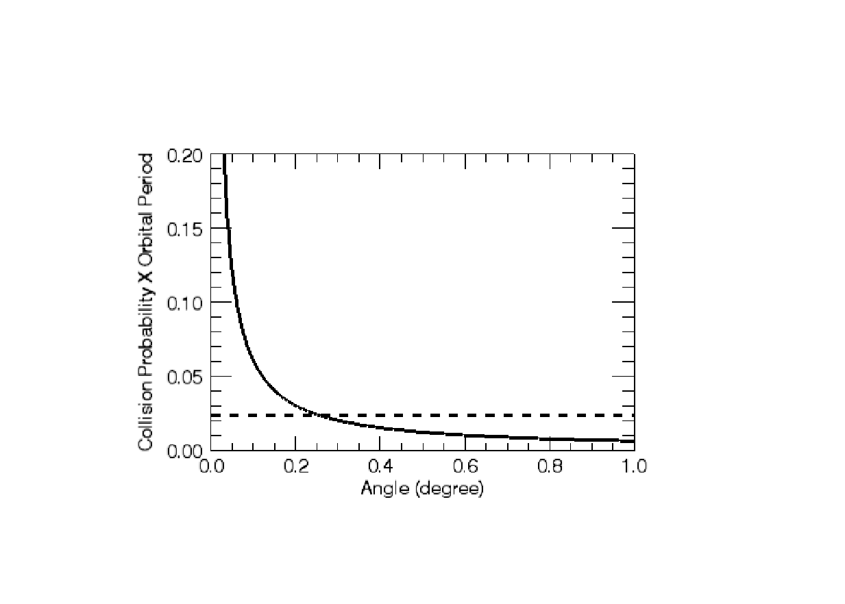
In practical Monte-Carlo type numerical simulations with a moderate number of particles, the number of cases of MOID is often statistically too small to accurately calculate the integrated impact flux of a projectile population on a given target. For computational efficiency, an artificially enhanced collision radius, with , can be adopted and the results scaled to the real collision radius [9, e.g.]. For the case of non-tangential encounters, the number of random orbits having MOID on the target orbit increases linearly with . As the collision probability itself also linearly increases with (Equation 13), the total impact flux is proportional to . Thus, the numerically computed impact flux with an adopted collision radius can be rescaled by a factor to obtain the real impact flux.
On the other hand, for the case of tangential encounters, the number of cases of MOID is proportional to . In practice, however, the exactly tangential cases are of measure zero, so two velocity vectors will not be strictly parallel near the MOID location, and there would be a small, non-zero angle between them. We can identify the near-tangential cases, i.e., those with , and in these cases the minimum encounter distance should be measured along the direction. The number of such cases having MOID is proportional to . As the collision probability in these encounters is proportional to (Equation 36), the integrated impact flux of these cases is proportional to . Therefore, in Monte-Carlo type numerical simulations, care should be taken with the artificially enhanced collision radius: the transition angle should be calculated with the physical radius (including a gravitational focusing factor), not the artificially enhanced collision radius; and the impact flux of the near-tangential collisions should be rescaled by a factor .
V Case Study
In this section, we provide a case study of the impact flux of a synthetic population of NEOs on Earth to illustrate that the correct treatment of tangential encounters is crucial to determine the correct impact frequency. The orbital parameters, the mass and the physical radius of Earth are adopted and the impact frequency from test particles orbiting in Earth-like orbits is calculated. The test particles’ semimajor axes are chosen randomly from the range 1.1–1.2 AU; this range exceeds ten times the Hill radius of Earth, and avoids the co-orbital region of Earth. The eccentricities are chosen randomly from zero to 0.3, and inclinations from zero to 5 degrees relative to the ecliptic; these ranges are selected for more frequent near-tangential encounters. The arguments of perihelia and the longitudes of ascending node are randomly generated within the range zero to . For statistical analysis, we repeat the same simulation 100 times (making different realizations of the random orbital parameters in each case), and we report mean values and standard deviations of the impact counts below.
Using the code developed by Gronchi [6], we determine that the total number of orbit crossings having local minimum distances smaller than the collision radius is . For the collision radius, we multiply the physical radius of Earth by the gravitational focusing factor of each test particle. For this synthetic population of impactors with Earth-like orbits, the mean of the gravitational focusing factor is a significantly large value of 2.96.

The total impact frequency calculated from Equation 13 varies greatly from simulation to simulation, from a minimum of 1.6 impacts per year to the maximum of 456 impacts per year; the results are shown in the gray shaded histogram in Figure 8. The mean value and the standard deviation are 9.8 and 47, respectively. This highly variable impact frequency is owed to the divergence of Equation 13 when test particles sporadically encounter Earth at nearly tangential velocities with . A careful examination of the distribution of the close encounters reveals that, among the local minimum distances smaller than the collision radius, only of them have smaller than the critical value (Equation 38), but the smallest case alone contributes more than 50 percent of the total impact frequency in 18 simulations out of 100. However, the corrected total impact frequency, when Equation 13 is replaced by Equation 37 for the near-tangential encounters, is found to be a very stable quantity, impacts per year (shown in the narrow black histogram on the left of Figure 8). These results show that the incorrect treatment of near-tangential encounters leads to systematically higher impact rate estimates and also greater scatter of the estimates.
In order to demonstrate the validity of our formulas for the impact probability in near-tangential encounters (Equation 37), we sampled 1000 test particle orbits having , from amongst the above-described synthetic populations of NEOs. We numerically integrated these particles with SWIFT-RMVS3 (http://www.boulder.swri.edu/~hal/swift.html), in a model including the Sun and the Earth with their actual mass and radius. The mean anomalies of the test particles were randomly generated in 10 different realizations, and 10 different numerical simulations are carried out for statistical analysis. We limited the orbit integration time to 10 years to avoid orbit evolution of the particles, and we adopted an integration step size of 1.4 minutes to accurately resolve collisions. From the 10 different numerical integrations, we find an average of impacts. We can compare this result of the numerical integrations with the expected number of impacts calculated with the unmodified Öpik-Wetherill formulas and with our corrected formulas. For the former, the expected value calculated from Equation 13 is 1802 impacts over ten years; this large value, which is unsurprising due to the nature of the singularity in Equation 13 for near-tangential encounters, is strongly in disagreement with the numerical integration result. For the latter, the expected value calculated from Equation 37 is 8 impacts over ten years, which is within 1– of the numerical integration result.
VI Summary
The classical method of Öpik [12] and Wetherill [17] for calculating collision probabilities of pairs of objects in Keplerian orbits has been widely used in many problems in planetary dynamics. In this paper, we have given a simplified derivation of the backbone of these calculations. Our derivation is easier to understand and to relate to the underlying geometry of collisions of Keplerian orbits. Additionally, our formula for the collision probability per unit time, (Equation 13), is explicitly commutative between the two colliding orbits (in contrast with the Öpik-Wetherill formulas).
We also derived the collision probability for tangential encounters (Equation 37); this regularizes a singularity in the Öpik-Wetherill formulas. We achieve this regularization by replacing the linear approximation in the vicinity of the collision point with a parabolic approximation of the true motions of the bodies, but otherwise the derivation is similar to the derivation for the non-tangential encounters. In the Appendix, we provide an alternate, fully analytic derivation, which additionally identifies the domain of applicability of the regularized collision probability of tangential collisions. Stated qualitatively, our formulas are valid in the regime in which the collision radius is much smaller than the heliocentric distance and the encounter velocity is not a vanishingly small fraction of the orbital velocity. The quantitative condition is described in detail in the Appendix.
The domains of the non-tangential and near-tangential collisions should be chosen based on the critical angle we derived in Section IV. The additional step needed in computing collision rates is not computationally expensive by virtue of the large increase in available computing power since the 1960s. The neglect of near-tangential encounter cases has the potential to lead to erroneous results; we demonstrated this by an exemplary, although extreme, case of the collision rates on Earth of a population of particles in Earth-like orbits.
Appendix A Appendix: Alternative Derivation for Tangential Collisions
In this appendix, we present an alternative derivation for for tangential collisions. The notation used is the same as in Section III, with a few exceptions as noted.
A.1 Derivations for Intersecting Orbits
Let us set up a coordinate system with origin at the point of intersection of the two orbits, the XY plane is the common orbital plane of the two orbits, and the X direction is radially outward from the Sun as in Section II.1. In general, the minimum distance between the center-of-figure of the two bodies is not zero and it does not occur at the point of intersection of the two orbits. Unlike Section III.1, let us assume that body 2 passes the origin at time with velocity , and body 1 passes the origin a time with velocity . (Note that here may be negative, if body 1 passes the origin before body 2.) At some time , the two bodies achieve a minimum mutual distance. For tangential encounters, we can write (without loss of generality)
| (A1) |
In the vicinity of the origin, we can approximate the motion of body 1 and body 2 as follows,
| (A2) | |||||
| (A3) |
Then the square of the distance between the two bodies can be expressed as a function of time,
| (A4) |
The minimum of the mutual distance occurs at , which can be obtained by the condition .
| (A5) | |||||
where is defined as
| (A6) |
Then the minimum distance occurs at
| (A7) |
where
| (A8) |
It is useful to compute
Then, setting in Eq. A4, we find
| (A9) |
For collision to occur, we must have , where is the collision radius. Thus, collision will occur provided , where is given by
| (A10) |
Recall that (Eq. A6), therefore Eq. A10 presents a quartic equation for , whose exact analytic solution is possible but tedious. Provided that , we obtain the leading order solution,
| (A11) |
A better approximation can be achieved by plugging the first approximation, Equation A11, into Equation A10, to obtain the leading order correction; this yields
| (A12) |
These two equations above are equivalent to Equation 27 and 28.
The condition requires that the change, , in the heliocentric velocity of the bodies over the time is much smaller than the encounter velocity, . We note that, using this approximate solution in Eq. A6 we have
| (A13) |
where is the average transverse velocity of the two bodies at the collision point, and we used ( is the heliocentric distance at the collision point, and is the heliocentric circular velocity). Thus, the condition is equivalent to
| (A14) | |||||
| (A15) |
In words, we can state the condition as: the collision radius (as a fraction of the heliocentric distance) is much smaller than the velocity difference (as a fraction of the orbital velocity). In physical terms, we can describe this as the condition that the collision radius should be much smaller than the heliocentric distance, when the velocity difference is not a vanishingly small fraction of the orbital velocity.
A.2 Derivations for Non-intersecting Orbits
For the case of non-intersecting orbits, we note that at the location of the MOID, the tangent to each orbit is normal to the relative distance vector, . We assume that the minimum mutual distance occurs in the vicinity of the MOID location. Let’s choose as origin that point on body 1’s orbit where the MOID occurs, and let’s choose the plane of body 1 as the XY plane.
Let’s assume that body 2 passes the MOID location, , at time with velocity and that body 1 passes the origin at some time later, with velocity . Then, for near-tangential encounters we can write,
| (A16) | |||||
| (A17) |
We can also express the time-dependent positions of body 1 and body 2 as follows.
| (A18) | |||||
| (A19) |
Then the distance between the two bodies is
| (A20) | |||||
The minimum of the mutual distance occurs at , which can be obtained by the condition . First, we derive
| (A21) | |||||
| (A22) |
where is given by Eq. A6. Then, we find
| (A23) |
It is useful to compute
We use Eq. A23 in Eq. A20 to find that the minimum distance:
| (A24) | |||||
where
| (A25) |
In a similar way to Equation A13, the small parameter can be understood as
| (A26) |
where is the average velocity of the two bodies. Because , we see that is of order .
Setting , we obtain a polynomial equation for :
| (A27) |
This is a polynomial of the 6th degree in . Keeping only the leading order terms, we need only solve a quadratic in :
| (A28) |
Only one of the two solutions is physical; we find
| (A29) |
which is the same as Equation 36.
References
- [1] Bottke, W. F., D. D. Durda, D. Nesvorný, R. Jedicke, A. Morbidelli, D. Vokrouhlický, and H. Levison 2005. The fossilized size distribution of the main asteroid belt. Icarus 175, 111–140.
- [2] Bottke, W. F., and R. Greenberg 1993. Asteroidal collision probabilities. Geophys. Res. Lett. 20, 879–881.
- [3] Dones, L., B. Gladman, H. J. Melosh, W. B. Tonks, H. F. Levison, and M. Duncan 1999. Dynamical Lifetimes and Final Fates of Small Bodies: Orbit Integrations vs Öpik Calculations. Icarus 142, 509–524.
- [4] Greenberg, R. 1982. Orbital interactions - A new geometrical formalism. AJ 87, 184–195.
- [5] Greenberg, R., A. Carusi, and G. B. Valsecchi 1988. Outcomes of planetary close encounters - A systematic comparison of methodologies. Icarus 75, 1–29.
- [6] Gronchi, G. F. 2005. An Algebraic Method to Compute the Critical Points of the Distance Function Between Two Keplerian Orbits. Celestial Mechanics and Dynamical Astronomy 93, 295–329.
- [7] Harris, A. W., and G. D’Abramo 2015. The population of near-Earth asteroids. Icarus 257, 302–312.
- [8] Ivanov, B. A. 2001. Mars/Moon Cratering Rate Ratio Estimates. Space Sci. Rev. 96, 87–104.
- [9] JeongAhn, Y., and R. Malhotra 2015. The current impact flux on Mars and its seasonal variation. Icarus 262, 140–153.
- [10] Liou, J.-C. 2006. Collision activities in the future orbital debris environment. Advances in Space Research 38, 2102–2106.
- [11] Moses, J. I., K. Rawlins, K. Zahnle, and L. Dones 1999. External Sources of Water for Mercury’s Putative Ice Deposits. Icarus 137, 197–221.
- [12] Öpik, E. J. 1951. Collision probabilities with the planets and the distribution of interplanetary matter. Proc. R. Irish Acad. Sect. A, vol. 54, p. 165-199 (1951). 54, 165–199.
- [13] Pokorný, P., and D. Vokrouhlický 2013. Öpik-type collision probability for high-inclination orbits: Targets on eccentric orbits. Icarus 226, 682–693.
- [14] Rickman, H., T. Wiśniowski, P. Wajer, R. Gabryszewski, and G. B. Valsecchi 2014. Monte Carlo methods to calculate impact probabilities. A&A 569, A47.
- [15] Southworth, J., T. C. Hinse, M. Dominik, M. Glitrup, U. G. Jørgensen, C. Liebig, M. Mathiasen, D. R. Anderson, V. Bozza, P. Browne, M. Burgdorf, S. Calchi Novati, S. Dreizler, F. Finet, K. Harpsøe, F. Hessman, M. Hundertmark, G. Maier, L. Mancini, P. F. L. Maxted, S. Rahvar, D. Ricci, G. Scarpetta, J. Skottfelt, C. Snodgrass, J. Surdej, and F. Zimmer 2009. Physical Properties of the 0.94-Day Period Transiting Planetary System WASP-18. ApJ 707, 167–172.
- [16] Vokrouhlický, D., P. Pokorný, and D. Nesvorný 2012. Öpik-type collision probability for high-inclination orbits. Icarus 219, 150–160.
- [17] Wetherill, G. W. 1967. Collisions in the Asteroid Belt. J. Geophys. Res. 72, 2429.
- [18] Wetherill, G. W. 1990. Formation of the earth. Annual Review of Earth and Planetary Sciences 18, 205–256.