Weak phonon-mediated pairing in BiS₂ superconductor from first principles

We calculated the phonon dispersion in the tetragonal unit cell using density functional perturbation theory on a sampling of the Brillouin zone of $4\times 4\times 2$ q-points with quantum espresso. Hereafter we refer to the phonon wave number by q. The obtained dispersion features a structural instability which extends all along the $\Gamma$-M line, matching previous studies.

In order to test the robustness of this instability, both to other approximations and to the inclusion spin-orbit coupling, we recalculated this dispersion using an all-electron calculation with and without spin-orbit coupling, and a q-grid of $2\times 2\times 1$ points. This yielded two dispersions, which are similar, with a slightly reduced depth of the imaginary frequencies from $-20$ meV to $-14$ meV. This confirms that this instability is robust.

We obtained the fully relaxed structure by using a unit cell of dimensions $\sqrt{2}a\times\sqrt{2}a$ where $a$ is the unit cell parameter of the tetragonal structure. For convenience we call this new crystal structure the $\sqrt{2}\times\sqrt{2}$ structure.

We calculated the phonon dispersion in this $\sqrt{2}\times\sqrt{2}$ structure (Figure 1). The obtained dispersion does not feature the instability ¹¹ 1 We find imaginary modes in the small region around the Gamma point, which could be due to insufficient energy cutoff for charge density.. We therefore use this structure to calculate electron-phonon coupling coefficients.

The effect of electron-phonon coupling on conventional superconductivity is well represented by the Eliashberg function [57]:

where $\omega$ is the frequency, $n$ and $n^{\prime}$ run over electronic bands, $\nu$ over phononic bands, k and q over the Brillouin zone, and $g$ are the electron-phonon coupling coefficients. Integrating the Eliashberg function over frequency gives the electron-phonon coupling factor $\lambda$:

The characteristic phonon frequency $\omega_{ln}$ is defined by:

The effects of the electron-phonon coupling on $T_{c}$ are well quantified by the McMillan-Allen-Dynes formula [58, 59]:

where $\mu^{*}$ is an adjustable pseudopotential parameter representing the effective electron-electron Coulomb repulsion suppressing the pairing instability [60].

In practice, the integration of equation 1 is carried out by approximating the singular delta function by a smeared function $\tilde{\delta}$ such as the Hermite-Gaussian [61]. However, this treatment can introduce two types of quantitative errors. First, the integrated value converged with respect to the $k$-point density suffers from a systematic error due to the width of the smearing function. Second, the convergence with respect to the $k$-point density tends to be very difficult to achieve, especially when the smearing width is small.

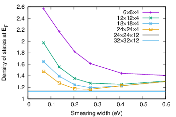
The magnitude of the error is well quantified by examining the electronic density of states $N(E)=\sum_{n\textbf{k}}\delta(E-\epsilon_{n\textbf{k}})$. We define $\tilde{N}$ as the density of states calculated using this smearing scheme. Here and hereafter, the functions and values with tilde denote the ones calculated with the smearing scheme. Equation 1 indicates that $\tilde{\alpha}^{2}F$ scales with $\tilde{N}(\tilde{E}_{F})^{2}$ in the limit where the electron-phonon coupling coefficients $g$ are independent of $n$, $n^{\prime}$, k and q ²² 2 In the Phonon package of quantum espresso, the prefactor $1/N(E_{F})$ in equation 1 is replaced by $1/\tilde{N}(E_{F})$, hence in this case we only obtain a $\tilde{N}(E_{F})$ dependence when summing the delta functions.. To estimate the impact of the above quantitative errors, we examined the dependence of the electronic density of states at the Fermi energy $\tilde{N}(\tilde{E}_{F})$ with respect to the smearing width and $k$-point grid (Figure 3). We obtained a well-converged value for $N(E_{F})$ using a very dense $k$-point grid and the tetrahedron integration method, which we refer to as the “exact” $N(E_{F})$ hereafter. We found that $\tilde{N}(\tilde{E}_{F})$ differs from the exact value by approximately 20% at the Gaussian width 0.5 eV, which is within a standard range of the width. Moreover, we found slowly convergent behaviour for widths lower than 0.1 eV. Notably, the values of $\tilde{N}(\tilde{E}_{F})$ are systematically larger than the exact one, indicating that $\tilde{\alpha}^{2}F$ can suffer from systematic overestimation in this material.

In order to mitigate the above-mentioned overestimation we modified the $\alpha^{2}F$ formula in practice, following recent technical developments [62], and obtained the rescaled Eliashberg function ³³ 3 In the case of quantum espresso, because the program uses the prefactor $1/\tilde{N}(E_{F})$ in equation 1, we need to use the following formula: $\displaystyle\alpha^{2}F_{\text{resc}}(\omega)=$ $\displaystyle\frac{\sum_{\textbf{q}}\sum_{nn^{\prime}\textbf{k}}\delta(\epsilon_{n\textbf{k}+\textbf{q}}-E_{F})\delta(\epsilon_{n^{\prime}\textbf{k}}-E_{F})}{\sum_{\textbf{q}}\sum_{nn^{\prime}\textbf{k}}\tilde{\delta}(\epsilon_{n\textbf{k}+\textbf{q}}-\tilde{E}_{F})\tilde{\delta}(\epsilon_{n^{\prime}\textbf{k}}-\tilde{E}_{F})}$ $\displaystyle\times\frac{\tilde{N}(\tilde{E}_{F})}{N(E_{F})}\tilde{\alpha^{2}F}(\omega)$ (5) :

The numerator is replaced to the exact $N(E_{F})^{2}$ since it corresponds to the dense k and q-points limit. Note that regardless of the k-point density, this modified formula gives us the exact value in the limit where the electron-phonon coupling coefficients $g$ are independent of $n$, $n^{\prime}$, k and q. With this formula, as shown in figure 4, we obtained values of $\lambda$ almost independent of the smearing width.

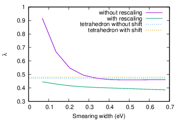
We confirmed these results by calculating $\alpha^{2}F$ with the optimized tetrahedron method [63] (Figure 2). We used four different q-point meshes, two with $3\times 3\times 3$ points (and a $18\times 18\times 6$ k-point mesh) and two with $4\times 4\times 2$ points (and a $24\times 24\times 4$ k-point mesh), one shifted along the $z$ axis and the other along all the axes ⁴⁴ 4 The unshifted q-mesh cannot be employed for the tetrahedron integration since it suffers from numerical divergence at $\textbf{q}=0$. Note that this is an artefact due to the discretisation and can be avoided if the q-point integral around $\textbf{q}=0$ is calculated analytically⁵⁵ 5 We have also employed the rescaling formula (Equation (6)) for $\alpha^{2}F_{tetra}$ to accelerate the k-point convergence. In this case, the denominator of the prefactor is calculated with the k and q-point mesh employed for the integration in equation (1).. We name $\alpha^{2}F_{\text{tetra}}$ the Eliashberg function obtained using the all-shifted $4\times 4\times 2$ q-point mesh. We obtained $\lambda=0.39$ and $\lambda=0.58$ for the first sampling, with $z$-shifted and all-shifted meshes, respectively, and $\lambda=0.48$ and $\lambda=0.47$ for the second sampling. The values obtained with $3\times 3\times 3$ points differ clearly, indicating a lack of convergence, while the ones obtained with $4\times 4\times 2$ points are both very close and between the two previous ones. This indicates a strong convergence. Moreover, the values obtained with the $4\times 4\times 2$ q-point mesh match closely the values obtained by integrating $\alpha^{2}F_{\text{resc}}$ in the limit of small smearing (Figure 4), which is the exact limit. The small deviation between the values of $\lambda$ indicates that the converged $\lambda$ is about or below 0.5.

The results obtained for $\omega_{ln}$ are less conclusive: indeed the values obtained for the two $3\times 3\times 3$ q-point grids are 116 K and 153 K, while the ones obtained using the two $4\times 4\times 2$ q-point grids are 98 K and 143 K. Let us note that $T_{c}$ is affected exponentially by $\lambda$ whereas it is affected only linearly by $\omega_{ln}$ (Equation (3)), which means that the convergence of $\lambda$ gives us the order of magnitude of $T_{c}$. In the following subsection, we show that this order of magnitude is clearly different from the one observed experimentally.

We calculated the superconducting transition temperature ($T_{c}$) of LaO_0.5F_0.5BiS₂ using density functional theory for superconductors ⁶⁶ 6 We sampled the Brillouin zone and the different bands using a weighted random set of points [40]. The standard error on the value of the gap was found to be 18.3%.. We ran a “static” calculation which only uses the zero frequency dielectric function, and a “dynamical” calculation which uses the full frequency-dependent dielectric function, both calculated using a $4\times 4\times 2$ k-point grid. We used $\alpha^{2}F_{\text{tetra}}$ in both calculations. The results are summarised in table 1.

It is interesting to compare this result to the output of the McMillan-Allen-Dynes formula [58]. We calculated $T_{c}$ with this formula using the parameters corresponding to $\alpha^{2}F_{\text{tetra}}$ for a large range of values of $\mu^{*}$. We then can obtain the $\mu^{*}$ corresponding to the value of $T_{c}$ calculated using density functional theory for superconductors. We obtain values of $\mu^{*}$ larger than in most conventional superconductors [64, 65] (Table 1). This is reminiscent of other ab-initio studies of superconductors [65].

The value of $T_{c}$ calculated here are very distant from all the values of $T_{c}$ measured in this compound, which are between 2.5 and 11.5 K [17]. We therefore conclude that conventional phonon-coupling superconductivity cannot explain the experimental data on LaO_0.5F_0.5BiS₂.

References

- [1] Y. Mizuguchi, H. Fujihisa, Y. Gotoh, K. Suzuki, H. Usui, K. Kuroki, S. Demura, Y. Takano, H. Izawa, and O. Miura, Phys. Rev. B 86, 220510 (2012a).
- [2] Y. Mizuguchi, S. Demura, K. Deguchi, Y. Takano, H. Fujihisa, Y. Gotoh, H. Izawa, and O. Miura, J. Phys. Soc. Japan 81, 114725 (2012b), .
- [3] V. P. S. Awana, A. Kumar, R. Jha, S. K. Singh, A. Pal, Shruti, J. Saha, and S. Patnaik, Solid State Commun. 157, 21 (2013).
- [4] H. Usui, K. Suzuki, and K. Kuroki, Phys. Rev. B 86, 220501 (2012).
- [5] H. Usui and K. Kuroki, Nov. Supercond. Mater. 1, 27 (2015), .
- [6] C. Morice, E. Artacho, S. E. Dutton, D. Molnar, H.-J. Kim, and S. S. Saxena, J. Phys. Condens. Matter 27, 135501 (2015).
- [7] J. Xing, S. Li, X. Ding, H. Yang, and H.-H. Wen, Phys. Rev. B 86, 214518 (2012).
- [8] R. Jha and V. P. S. Awana, J. Supercond. Nov. Magn. 27, 1 (2013), .
- [9] S. Demura, Y. Mizuguchi, K. Deguchi, H. Okazaki, H. Hara, T. Watanabe, S. J. Denholme, M. Fujioka, T. Ozaki, H. Fujuhisa, Y. Gotoh, O. Miura, T. Yamaguchi, H. Takeya, and Y. Takano, J. Phys. Soc. Japan 82, 033708 (2013).
- [10] R. Jha, A. Kumar, S. Kumar Singh, and V. P. S. Awana, J. Supercond. Nov. Magn. 26, 499 (2013).
- [11] H.-F. Zhai, Z.-T. Tang, H. Jiang, K. Xu, K. Zhang, P. Zhang, J.-K. Bao, Y.-L. Sun, W.-H. Jiao, I. Nowik, I. Felner, Y.-K. Li, X.-F. Xu, Q. Tao, C.-M. Feng, Z.-A. Xu, and G.-H. Cao, Phys. Rev. B 90, 64518 (2014).
- [12] D. Yazici, K. Huang, B. D. White, A. H. Chang, A. J. Friedman, and M. B. Maple, Philos. Mag. 93, 673 (2013).
- [13] X. Wan, H.-C. Ding, S. Y. Savrasov, and C.-G. Duan, Phys. Rev. B 87, 115124 (2013).
- [14] T. Yildirim, Phys. Rev. B 87, 20506 (2013).
- [15] C. Morice, E. Artacho, S. E. Dutton, H.-J. Kim, and S. S. Saxena, J. Phys. Condens. Matter 28, 345504 (2016), .
- [16] R. Higashinaka, T. Asano, T. Nakashima, K. Fushiya, Y. Mizuguchi, O. Miura, T. D. Matsuda, and Y. Aoki, J. Phys. Soc. Japan 84, 023702 (2015), .
- [17] Y. Mizuguchi, T. Hiroi, J. Kajitani, and H. Takatsu, J. Phys. Soc. Japan 83, 053704 (2014).
- [18] J. Zhang, K. Huang, Z. F. Ding, D. E. MacLaughlin, O. O. Bernal, P. C. Ho, C. Tan, X. Liu, D. Yazici, M. B. Maple, and L. Shu, 2, 1 (2016), .
- [19] K. Deguchi, Y. Mizuguchi, S. Demura, H. Hara, T. Watanabe, S. J. Denholme, M. Fujioka, H. Okazaki, T. Ozaki, H. Takeya, T. Yamaguchi, O. Miura, and Y. Takano, Europhys. Lett. 101, 17004 (2013).
- [20] J. Kajitani, K. Deguchi, A. Omachi, T. Hiroi, Y. Takano, H. Takatsu, H. Kadowaki, O. Miura, and Y. Mizuguchi, Solid State Commun. 181, 1 (2014), .
- [21] I. Pallecchi, G. Lamura, M. Putti, J. Kajitani, Y. Mizuguchi, O. Miura, S. Demura, K. Deguchi, and Y. Takano, Phys. Rev. B 89, 1 (2014).
- [22] C. T. Wolowiec, D. Yazici, B. D. White, K. Huang, and M. B. Maple, Phys. Rev. B 88, 064503 (2013), .
- [23] T. Tomita, M. Ebata, H. Soeda, H. Takahashi, H. Fujihisa, Y. Gotoh, Y. Mizuguchi, H. Izawa, O. Miura, S. Demura, K. Deguchi, and Y. Takano, J. Phys. Soc. Japan 83, 063704 (2014), .
- [24] H. Kotegawa, Y. Tomita, H. Tou, H. Izawa, Y. Mizuguchi, O. Miura, S. Demura, K. Deguchi, and Y. Takano, J. Phys. Soc. Japan 81, 103702 (2012).
- [25] J. Lee, M. B. Stone, A. Huq, T. Yildirim, G. Ehlers, Y. Mizuguchi, O. Miura, Y. Takano, K. Deguchi, S. Demura, and S. H. Lee, Phys. Rev. B 87, 205134 (2013), .
- [26] A. Athauda, J. Yang, S. Lee, Y. Mizuguchi, K. Deguchi, Y. Takano, O. Miura, and D. Louca, Phys. Rev. B 91, 1 (2015), .
- [27] L. K. Zeng, X. B. Wang, J. Ma, P. Richard, S. M. Nie, H. M. Weng, N. L. Wang, Z. Wang, T. Qian, and H. Ding, Phys. Rev. B 90, 1 (2014), .
- [28] Z. R. Ye, H. F. Yang, D. W. Shen, J. Jiang, X. H. Niu, D. L. Feng, Y. P. Du, X. G. Wan, J. Z. Liu, X. Y. Zhu, H.-H. Wen, and M. H. Jiang, Phys. Rev. B 90, 045116 (2014).
- [29] K. Terashima, J. Sonoyama, T. Wakita, M. Sunagawa, K. Ono, H. Kumigashira, T. Muro, M. Nagao, S. Watauchi, I. Tanaka, H. Okazaki, Y. Takano, O. Miura, Y. Mizuguchi, H. Usui, K. Suzuki, K. Kuroki, Y. Muraoka, and T. Yokoya, Phys. Rev. B 90, 1 (2014), .
- [30] T. Sugimoto, D. Ootsuki, C. Morice, E. Artacho, S. S. Saxena, E. F. Schwier, M. Zheng, Y. Kojima, H. Iwasawa, K. Shimada, M. Arita, H. Namatame, M. Taniguchi, M. Takahashi, N. L. Saini, T. Asano, R. Higashinaka, T. D. Matsuda, Y. Aoki, and T. Mizokawa, Phys. Rev. B 92, 041113 (2015), .
- [31] G. B. Martins, A. Moreo, and E. Dagotto, Phys. Rev. B 87, 81102 (2013).
- [32] T. Zhou and Z. D. Wang, J. Supercond. Nov. Magn. 26, 2735 (2013).
- [33] X. Wu, J. Yuan, Y. Liang, H. Fan, and J. Hu, Europhys. Lett. 108, 27006 (2014).
- [34] Y. Liang, X. Wu, W.-F. Tsai, and J. Hu, Front. Phys. 9, 194 (2014).
- [35] B. Liu and S. Feng, Europhys. Lett. 106, 17003 (2014).
- [36] Y. Yang, W. S. Wang, Y. Y. Xiang, Z. Z. Li, and Q.-H. Wang, Phys. Rev. B 88, 1 (2013), .
- [37] B. Li, Z. W. Xing, and G. Q. Huang, Europhys. Lett. 101, 47002 (2013).
- [38] Y. Feng, H.-C. Ding, Y. Du, X. Wan, B. Wang, S. Y. Savrasov, and C.-G. Duan, J. Appl. Phys. 115, 5 (2014), .
- [39] M. Lüders, M. A. L. Marques, N. N. Lathiotakis, A. Floris, G. Profeta, L. Fast, A. Continenza, S. Massidda, and E. K. U. Gross, Phys. Rev. B 72, 1 (2005), .
- [40] M. A. L. Marques, M. Lüders, N. N. Lathiotakis, G. Profeta, A. Floris, L. Fast, A. Continenza, E. K. U. Gross, and S. Massidda, Phys. Rev. B 72, 1 (2005), .
- [41] P. Giannozzi, S. Baroni, N. Bonini, M. Calandra, R. Car, C. Cavazzoni, D. Ceresoli, G. L. Chiarotti, M. Cococcioni, I. Dabo, A. Dal Corso, S. de Gironcoli, S. Fabris, G. Fratesi, R. Gebauer, U. Gerstmann, C. Gougoussis, A. Kokalj, M. Lazzeri, L. Martin-Samos, N. Marzari, F. Mauri, R. Mazzarello, S. Paolini, A. Pasquarello, L. Paulatto, C. Sbraccia, S. Scandolo, G. Sclauzero, A. P. Seitsonen, A. Smogunov, P. Umari, and R. M. Wentzcovitch, J. Phys. Condens. Matter 21, 395502 (2009), .
- [42] “http://elk.sourceforge.net,” (2004).
- [43] J. P. Perdew and A. Zunger, Phys. Rev. B 23, 5048 (1981), .
- [44] D. D. Koelling and B. N. Harmon, J. Phys. C Solid State Phys. 10, 3107 (1977).
- [45] A. Migdal, JETP Lett. 34, 996 (1958).
- [46] G. M. Eliashberg, Sov. Phys. JETP 11, 696 (1960).
- [47] G. M. Eliashberg, Sov. Phys. JETP 12, 1000 (1961).
- [48] N. D. Mermin, Phys. Rev. 137, A1441 (1965).
- [49] A. Görling and M. Levy, Phys. Rev. A 50, 196 (1994).
- [50] R. Akashi and R. Arita, Phys. Rev. B 88, 14514 (2013a).
- [51] S. Baroni, S. de Gironcoli, A. Dal Corso, and P. Giannozzi, Rev. Mod. Phys. 73, 515 (2001).
- [52] W. E. Pickett, Phys. Rev. B 26, 1186 (1982).
- [53] R. Akashi and R. Arita, Phys. Rev. Lett. 111, 57006 (2013b).
- [54] R. Akashi and R. Arita, J. Phys. Soc. Japan 83, 061016 (2014), .
- [55] R. Akashi, M. Kawamura, S. Tsuneyuki, Y. Nomura, and R. Arita, Phys. Rev. B 91, 224513 (2015), .
- [56] Y. Takada, J. Phys. Soc. Japan 45, 786 (1978).
- [57] D. Scalapino, Superconductivity, Vol. 1, edited by R. Parks (Dekker, New York, 1969) p. 449.
- [58] W. L. McMillan, Phys. Rev. 167, 331 (1968).
- [59] P. B. Allen and R. C. Dynes, Phys. Rev. B 12, 905 (1975).
- [60] P. Morel and P. W. Anderson, Phys. Rev. 125, 1263 (1962).
- [61] M. Methfessel and A. T. Paxton, Phys. Rev. B 40, 3616 (1989).
- [62] T. Koretsune and R. Arita, (2016), arXiv:1610.09441 .
- [63] M. Kawamura, Y. Gohda, and S. Tsuneyuki, Phys. Rev. B - Condens. Matter Mater. Phys. 89, 1 (2014), .
- [64] J. P. Carbotte, Rev. Mod. Phys. 62, 1027 (1990).
- [65] R. Akashi, K. Nakamura, R. Arita, and M. Imada, Phys. Rev. B 86, 054513 (2012).