Bayesian Non-Homogeneous Markov Models via Polya-Gamma Data Augmentation with Applications to Rainfall Modeling
Discrete-time hidden Markov models are a broadly useful class of latent-variable models with applications in areas such as speech recognition, bioinformatics, and climate data analysis. It is common in practice to introduce temporal non-homogeneity into such models by making the transition probabilities dependent on time-varying exogenous input variables via a multinomial logistic parametrization. We extend such models to introduce additional non-homogeneity into the emission distribution using a generalized linear model (GLM), with data augmentation for sampling-based inference. However, the presence of the logistic function in the state transition model significantly complicates parameter inference for the overall model, particularly in a Bayesian context. To address this we extend the recently-proposed Polya-Gamma data augmentation approach to handle non-homogeneous hidden Markov models (NHMMs), allowing the development of an efficient Markov chain Monte Carlo (MCMC) sampling scheme. We apply our model and inference scheme to 30 years of daily rainfall in India, leading to a number of insights into rainfall-related phenomena in the region. Our proposed approach allows for fully Bayesian analysis of relatively complex NHMMs on a scale that was not possible with previous methods. Software implementing the methods described in the paper is available via the R package NHMM.
, , and
University of California, Irvine?? and Columbia University??
1 Introduction
Consider the problem of modeling the dynamics of a multivariate discrete time series , with component measurements , , and a discrete-time index . A useful modeling approach in this context is the hidden Markov model (HMM), where the observed ’s are assumed to be a stochastic function of a (hidden) finite-state Markov process , with components , and where each vector is assumed to be conditionally independent of all other vectors and state variables , , given state (Zucchini, MacDonald and Langrock, 2016). The conditional distribution of the vectors at time given the state is often assumed to be time-homogeneous, defined by so-called emission distributions,11 1 Here we use the term “emission distributions”, widely used in speech recognition and language modeling (e.g., Jurafsky and Martin (2014)) - these are also referred to as “state-dependent distributions” (e.g., Zucchini, MacDonald and Langrock (2016)) where represents the emission distribution parameters. The distributional choice for will depend on the particular characteristics of the measurements for a given application.
HMMs are appealing for problems where the dynamics of are too complex to be directly modeled (e.g., for high-dimensional problems where is large) but can instead be approximated via a discrete-state hidden Markov process . For example, a common assumption in practice (and one that is used in this paper - see also Zucchini, MacDonald and Langrock (2016), p.140, and the discussion of contemporaneous conditional independence), is to assume that the components of are conditionally independent given the state, i.e., that , where denotes the conditional distribution of component of the observed vector . HMMs can also be used to produce a time-dependent clustering of the observations , where the state variables are interpreted as indicators of cluster memberships, with the Markov dependence providing temporal dependence (in contrast to mixture model clustering for example, where the cluster memberships are modeled as being independent). Using HMMs for clustering in this manner can be useful in econometric, ecological, or other scientific time-series applications (e.g., MacDonald and Zucchini (1997); Raphael (1999); Siepel and Haussler (2004); Mamon and Elliott (2007); Patterson et al. (2016)). The goal is often to try to gain insight into possible latent processes that might be giving rise to the observed data, for example by analyzing and interpreting differences among the emission distributions across states.
The time-homogeneity of the standard HMM (at the parameter level, as described above) can be limiting in practice, for example if has seasonal dependence or is non-stationary. One approach to relaxing this assumption is to allow the transition matrix probabilities to be dependent on an exogenous time-series , resulting in a non-homogeneous hidden Markov model (NHMM) (e.g., Hughes and Guttorp (1994); Diebold and Lee (1994); Hughes, Guttorp and Charles (1999); Kirshner, Smyth and Robertson (2004); Kim, Piger and Startz (2008); Paroli and Spezia (2008); Meligkotsidou and Dellaportas (2011); Rajagopalan, Lall and Tarboton (1996)). A natural parametrization is to model each of the rows of the transition matrix via a multinomial logistic function, with possible outcomes (the possible states at time given the current state ). Temporal inhomogeneity can also be introduced in the emission component of the model, for example by allowing the parameters of the emission distributions to vary with time and location as a function of another exogenous process (e.g., Holsclaw et al. (2016)) .


As a motivating example we consider the problem of modeling and simulating daily station rainfall data over India where the observations correspond to the amount of rain that has fallen on day at weather station . The data we analyze has been collected daily for 30 years at 63 rain gauge stations across India, totaling well over half a million observations (). The geographical area of interest contains diverse sub-regions where the rainfall varies greatly in seasonal timing and amount. As shown in Figure 1 some stations lie in the Himalayas while others are located variously in coastal, monsoon or desert regions; these data are not isotropic in nature. Figure 2 shows the rainy days in lighter shades indicating amounts and dry days in dark shades for three contrasting stations (see Holsclaw (2017) for additional stations).
Accurately modeling and simulating rainfall on a daily time scale is important across a number of diverse applications such as crop modeling, flood risk assessment, and water policy decisions (Hansen et al., 2006; Challinor et al., 2009; Piani et al., 2010). Multivariate HMMs have been successfully applied to this modeling problem in the past, where the hidden variables can be interpreted as weather states exhibiting persistence at daily time scales, and the emission distributions capture the spatial and distributional characteristics of observed rainfall for each state (Zucchini and Guttorp, 1991; Hughes and Guttorp, 1994; Kirshner, 2010; Greene, Robertson and Kirshner, 2008; Zucchini, MacDonald and Langrock, 2016). Of direct interest to climatologists is the situation where the rainfall in a given region is being influenced or driven by time-varying atmospheric variables such as pressure differentials at large spatial scales. Relating these large scale variables to local rainfall characteristics at particular station locations is known as downscaling. NHMMs have been found to be broadly useful in this context where the variables act as “drivers” for the Markov transition matrix as described earlier (Hughes, Guttorp and Charles, 1999; Bellone, Hughes and Guttorp, 2000; Charles et al., 2004; Robertson, 2009; Germain, 2010; Carey-Smith, Sansom and Thomson, 2014; Heaps, Boys and Farrow, 2015). Other work in a downscaling context, such as that of Berrocal, Gelfand and Holland (2010) and Fuentes and Raftery (2005) for ozone and airborne particulates, focuses on the use of Gaussian models - these models are not appropriate here given the non-negativity and non-Normality of precipitation data.
There are a multitude of other modeling approaches that could be used in this context. In particular, dynamic spatio-temporal models provide a rich framework for modeling spatial and temporal dependencies. These models often use continuous latent-space representation (in contrast to the discrete state representation of the HMM approach) and are often parametrized in a manner that can incorporate relevant scientific knowledge, e.g., in the form of differential equations (see Hooten and Wikle (2010), for a review). Such approaches can provide richer representations for spatial structure that go beyond the conditional independence assumption that has often been used when NHMMs are applied to precipitation modeling (and that we use here in this paper). In Section 5.4 and in Holsclaw (2017) we examine the model’s ability to capture spatial dependence across stations and conclude that while the conditional independence approach tends to underestimate the true spatial dependence, that the model nonetheless is capturing much of the dependence that is empirically observed. For applications where spatial dependence is of critical importance, additional spatial dependence could be incorporated in the emission component of our proposed model at the cost of additional complexity and computational effort.
Many of the early applications of HMMs and NHMMs, to climate data as well as to other problems, have relied on point estimates of model parameters, often using the Expectation-Maximization (EM) algorithm for parameter estimation (Dempster, Laird and Rubin, 1977). There is, however, a growing need for efficient Bayesian methods for assessing uncertainty in these types of models (e.g., Rydén (2008)). For example, in the context of climate data, modeling the uncertainty in rainfall amounts is important in both seasonal forecasting and climate change downscaling applications (Maraun et al., 2010; Vermeulen et al., 2013) and Bayesian simulations are better suited to characterizing such uncertainty than point-estimate approaches.
While there has been extensive development of Bayesian methods for HMMs (Scott, 2002; Frühwirth-Schnatter, 2006; Rydén, 2008; Patterson et al., 2016) there has been little work on Bayesian estimation of NHMMs. Prior work has typically focused on analysis of small univariate data sets due to the complexity and computational expense of the Metropolis-Hastings MCMC schemes used for inference (e.g., Filardo and Gordon (1998); Spezia et al. (2014)). Meligkotsidou and Dellaportas (2011) apply the Bayesian multinomial logit regression (MNL) latent variable technique developed by Holmes and Held (2006a); Holmes and Held (2006b) to the NHMM, illustrating the approach using a relatively small univariate financial econometrics data set with monthly observations over 38 years. For many applications however we need methods that scale up efficiently to much larger data sets. The rainfall data set we analyze later in the paper consists of a 63-dimensional time-series with observations per time-series.
The development of an efficient Bayesian sampling scheme to handle logistic transition matrices in NHMMs, a problem that has proven challenging in the past because of the lack of conjugacy that arises due to the logistic functional form. With scalability in mind we adopt the Polya-Gamma latent variable method previously used for sampling in a multinomial logistic (MNL) regression framework (Polson, Scott and Windle, 2013) and extend it to the NHMM in this paper. We are motivated by the results in Polson, Scott and Windle (2013) which showed that the Polya-Gamma latent variable method is significantly faster than alternative sampling schemes such as those of Holmes and Held (2006a) and Frühwirthh-Schnatter and Frühwirth (2007). Furthermore, because the Polya-Gamma method uses only Gibbs sampling steps this obviates the need for extensive parameter-tuning of the sampling algorithm, leading to a significantly simpler implementation in software compared to methods based on Metropolis-Hastings steps for example. We have implemented the algorithm proposed in this paper and made this model available in the NHMM R package on the Comprehensive R Archive Network (CRAN).
The contributions of our paper are as follows. We propose a novel hidden Markov model with inhomogeneity in both the transition and emission state-dependent distributions. This model generalizes earlier NHMMs that contained either transition or emission inhomogeneity but not both. An additional significant contribution of the paper is the development of a fully Bayesian estimation scheme for this class of models. In particular we develop a scalable Bayesian sampling scheme for the logistic transition component of the NHMM, enabling these methods to be applied to much larger data sets than in prior work. Finally we demonstrate the application of the model and the Bayesian inference algorithms to a large-scale multi-decadal precipitation data set.
Section 2 lays out the proposed Bayesian multivariate NHMM. A description of the Bayesian implementation of the MCMC algorithm and the handling of missing data, predictive simulations, and forecasting are discussed in Section 3; further modeling considerations such as variable selection and model choice for the NHMM are included in Appendix A. Local rainfall amounts for 63 stations in and around India and the exogenous variables to be downscaled are described in Section 4; specific details pertaining to the exogenous variables can be found in Appendix B. Section 4 also provides a brief summary of rainfall modeling. Section 5 includes the analysis and results of the NHMM when applied to the Indian rainfall data. Our findings and general conclusions are summarized in Section 6.
2 Bayesian Multivariate Non-Homogeneous Markov Model
2.1 The NHMM and the Likelihood
The observed multivariate time-series , with discrete-time index , is modeled using an NHMM. A general way to introduce exogenous dependence into the transition matrix is to allow each transition to have its own set of logistic coefficients (or at least of them, subject to identifiability), implying coefficients in total for exogenous variables. This was the approach taken in Meligkotsidou and Dellaportas (2011) for . However, this model requires a large number of parameters as grows. A more parsimonious approach (and the one we follow in this paper) is to have one set of regression coefficients for each state, with coefficients in total, allowing the probability of entering each state to be modulated by a set of weighted regressors (via the logistic link), but where the modulation is independent of the previous state (e.g., Kirshner, Smyth and Robertson (2004)). The intuitive interpretation is that the exogenous variables control how likely the Markov chain is to enter each state (via the logistic link and regression coefficients), and thus, as the exogenous variables change over time, so do the probabilities of being in each state. As a simple example, if one of the exogenous variables reflects seasonality (time of year), this allows the model to visit hidden states in a seasonal fashion. The hidden process is Markov with an inhomogeneous transition matrix with components , . The transition probability entries at time are modeled via a multinomial logistic link function:
| (1) |
where is a -dimensional exogenous covariate time series, and is a -dimensional vector of coefficients corresponding to the components of . For notational convenience let for all . We assign one of the to zero for some value of (one and a vector of for some j) for identifiability. The choice of the logistic function above is discussed further in Section 3.1.
The other main component of an NHMM is the set of state-dependent emission distributions , and where is the set of all parameters of the emission distribution. Each combination of state () and station () has its own emission distribution (for this particular application the emission distribution will be a zero-inflated mixture of exponential distributions.) In general these distributions can be specified to be inhomogeneous over time by allowing the parameters to depend on time-varying exogenous variables , yielding .
Figure 3 shows a graphical representation of the multivariate NHMM and how the two types of exogenous variables (,) impact the model. If the values of the latent variables are assumed to be known, the conditional likelihood for the model above can be expressed as:
| (2) |
where for is defined via an initial state distribution and where the transition probabilities are defined as in Equation 1. When the latent variables are unknown, the likelihood can be computed by marginalizing over the unknown values in the usual recursive manner for HMMs (e.g., see Scott (2002)). Priors and inference procedures for the unknown parameters and are described in the next section.
3 Bayesian Inference and MCMC Algorithm
We describe below how to perform inference in a Bayesian framework for the model in the preceding section using a Markov chain Monte Carlo (MCMC) algorithm. Posterior full conditional distributions can be computed for each of , , and independently, such that each step of the MCMC algorithm focuses on only one set of parameters at a time. Our primary emphasis below is on the development of a sampling method for the transition matrix parameters since this has traditionally presented difficulties in the context of Bayesian analysis of NHMMs and has effectively limited the sizes of data sets that can be analyzed in past studies.
If the posterior full conditional distributions are known in closed-form then the parameters can be sampled by Gibbs steps within the MCMC. For problems where the posterior distributions are not conjugate, it is sometimes possible to have auxiliary variable methods facilitate rendering full posterior conditional distributions in a form that can be sampled from. For the NHMM described above, two sets of latent variables can be added to the model: one set for sampling the coefficients associating with the transition probabilities of the hidden states (Polson, Scott and Windle, 2013) and another set associated with parameters of the emission distributions (Albert and Chib, 1993). Using auxiliary variables (and the resulting Gibbs sampling algorithm) in this manner can be more efficient compared to alternative approaches such as Metropolis-Hastings, e.g., leading in some cases to better mixing (and thus less thinning and fewer iterations) as well as having the advantage of not requiring tuning parameters for the sampler (i.e., which results in a user friendly R Package).
3.1 Sampling the Coefficients
In this NHMM, there are coefficients () associated with each of the observed daily variables . These coefficient parameters () are related to the transition probabilities associated with the hidden states through a link function. There are two standard link functions that are typically used in this context: the logistic multinomial (MNL) and the multinomial probit (MNP) (Riihimaki, Jylanki and Vehtari, 2013; Neal, 1997), both of which are commonly used in regression modeling of polychotomous response variables. Although there has been relatively little literature on Bayesian inference with MNP or MNL link functions for NHMMs, Bayesian implementations in the context of regression modeling are well-studied (e.g., see Albert and Chib (1993); Aitchison and Bennett (1970); Chib and Greenburg (1998); Imai and van Dyk (2005); McCulloch, Polson and Rossi (2000); Johndrow, Lum and Dunson (2013); Zhang, Boscardin and Belin (2008) for MNP regression and Holmes and Held (2006a); Holmes and Held (2006b); Scott (2011); Polson, Scott and Windle (2013); Frühwirth-Schnatter (2008); O’Brien and Dunson (2004) for MNL regression). Although mathematically quite similar (Paap and Frances, 2000) MNL and MNP require quite different Bayesian sampling algorithms. The Bayesian implementation of the MNP regression model usually samples the coefficients using latent variables; this is quite efficient and therefore works well for large data sets (Albert and Chib, 1993). However, unlike the regression case, the NHMM has the additional need to calculate the transition probabilities for which there is no analytic solution in the case of the MNP. For this reason the MNL has tended to be the link function of choice for NHMM modeling. But the Bayesian implementation of MNL tends to be slow, requiring multiple tuning parameters and long sampling runs. For this reason, it is often only used with relatively small data sets and small numbers of coefficients (Scott, 2011; Frühwirth-Schnatter, 2008; O’Brien and Dunson, 2004). For example, Meligkotsidou and Dellaportas (2011) construct a Bayesian NHMM inference procedure by drawing from the MNL regression method of Holmes and Held (2006a); Holmes and Held (2006b) using a relatively complex slice sampler to analyze a small univariate time series.
Polson, Scott and Windle (2013) has recently introduced a new MNL method using Polya-Gamma latent variables, providing an algorithm that is more efficient (both in terms of time per run and needing no tuning parameters), which opens up the possibility of handling much larger data sets with these models. This provides the motivation to apply the Polson, Scott and Windle (2013) Polya-Gamma MNL latent variable method to the NHMM. There are a number of aspects of the MNL regression method that are altered in the extension to the NHMM case (refer to Section 5 of Polson, Scott and Windle (2013) for details for sampling of the MNL regression). In the NHMM, there is no observed multinomial data as in MNL regression. Instead, the sampled hidden states are set up in matrix form to conform to the MNL regression method. is a by matrix with entries , where the columns contain the binary representation of the hidden states (a 1 in the column of the and 0 elsewhere) and is updated during each of the iterations of the MCMC sampler. The exogenous variables and the Markov dependence (from for ) are included in the matrix which has dimension by . The first columns encode the information of the Markov property () in a binary form followed by columns for the exogenous variables ( for all and ). is a by matrix of coefficients, indexed by where and . One of the rows of is set to zero for identifiability (the first by entries are the ’s and the next B columns are the ’s). The full conditional posterior distribution for the ’s allows them to be drawn conditioned on the current draw of hidden states and other variables. The likelihood for is given by:
| (3) |
where with (which is needed for the multinomial logistic form). is a set of latent variables with components . At each time step there is only one observation of the hidden state, so in terms of the MNL regression the observation count is one. The full conditional posteriors are given by:
where scalars and . is a T by T diagonal matrix containing along the diagonal. and are parameters of the conjugate prior; the implementation in our R package allows for a conjugate prior of the form . If a non-informative prior is desirable then we can let and be zero as we do in our rainfall example later in the paper.
The transition matrix is a necessary part of the NHMM, not typically used in MNL/MNP regression. Once the coefficients () are sampled then the transition probabilities can be easily obtained through the logistic relationship given in Equation 1. This leads to a K by K transition matrix for time :
where each row of sums to one.
3.2 Sampling the Hidden States, Conditioned on Parameters and
Conditioned on sampled values of the parameters and , and given the observed data and , the posterior full conditional distribution of the hidden state at the th sampling iteration is as follows (dropping the third subscript from the variables for clarity):
where is the emission distribution for state . Each of the are sampled in succession for all at each of the iterations of the larger MCMC algorithm. Without loss of generality, we assign the first hidden state, associated with day one of the time series, to state one: .
We can sample the hidden states using well-known efficient recursive techniques. For example, Scott (2002) describes two Bayesian algorithms for sampling the hidden state of an HMM: a forward-backward (FB) recursive algorithm and a direct Gibbs (DG) sampler. The FB method mixes more rapidly but takes more computational effort. We use the DG method, which can require more iterations (for better mixing) but is less expensive per iteration.
Finite mixture models, including NHMMs, can suffer from the issue of non-identifiability of the hidden states (Jasra, Holmes and Stephens, 2005; Spezia, 2009). Any pair of states could swap labels and the likelihood would remain invariant; leading to identical marginal posterior densities, see Frühwirth-Schnatter (2006) for a full discussion. Both Scott (2002) and Meligkotsidou and Dellaportas (2011) discuss this issue for similar HMM and NHMM models respectively. However, NHMMs are less likely to suffer from label switching compared to HMMs or finite mixtures due to the dependence of the latent states on fixed covariates, which effectively makes label-switching less likely for the states. In particular, for the model we propose in this paper, both the state transitions and the emission distribution parameters are dependent on fixed covariate time-series. In our experimental results with rainfall data (described in Section 5) we did not see any evidence of label switching.
3.3 Sampling for the Emission Distribution Parameters
For this application we model daily rainfall amounts by a zero-inflated mixture of two exponential distributions, an approach that has been found most effective in past work (Woolhiser and Roldan, 1982; Wilks, 1998; Wilks, 1999a; Wilks, 1999b; Ailliot et al., 2015). Other possible modeling options include zero-inflated Gamma distributions or mixtures of exponential, Normal, or Poisson distributions (Hay, 1991; Hughes and Guttorp, 1994; Charles, Bates and Hughes, 1999; Bellone, Hughes and Guttorp, 2000; Holsclaw et al., 2016). The zero-inflated mixture of two exponential distributions has a physical interpretation of its three components corresponding to no rain, light rain, and heavy rain. The delta function at zero () allows for zero inflation for additional dry days, and the light rain and heavy rain each have an exponential distribution, where:
| (4) |
where and for this application denotes the mixing probability parameters and rate parameters of the emission distributions. The mixing probabilities are assumed to be dependent on the exogenous variables and are modeled by a generalized linear model (GLM) through a probit link: for all ; provides the dependence on the hidden states, with and as the mean. Let for , , and ; let denote the parameters of the emission distributions. The are state dependent and function like a random effect whereas the are not state dependent thus allowing significance testing of the exogenous variable per station.
The probit link for ordered multinomial categories allows for the sampling of the coefficients to be done through the standard Bayesian data augmentation approach (Cox, 1971; McCullagh and Nelder, 1989; Albert and Chib, 1993). To allow for conjugate full conditional posterior distributions of the parameters of , we need to introduce two sets of latent variables ( and ). The first set of latent variables (with components taking values in the set ) facilitates calculations of . The emission distribution becomes:
where . A second set of latent variables with components is introduced to enable Gibbs sampling of . The latent variables are three ordered categories (no rain, light rain, and heavy rain) which, following the ordered multinomial probit algorithm in Albert and Chib (1993), requires one fixed break point (set to zero) and one unknown break point () (more categories would require more unknown breakpoints). The relationship between and is as follows:
This results in posterior full conditional distributions as described in Holsclaw et al. (2016). For our rainfall modeling application the and parameters are each given a low weight conjugate prior () (label switching does not occur because of the ordered nature of the latent variable method of Albert and Chib (1993).) The coefficients have non-informative priors as well (Albert and Chib, 1993). This setup leads to the parameters having closed form full conditional posterior distributions that can be sampled via Gibbs steps in the MCMC algorithm.
3.4 Missing Data Imputation
The missing data points can be treated as unknown random variables whose posterior distributions are inferred along with the other variables in the model. The posterior conditional distribution of each missing data point ( at time and station ) is given by: . Data that is missing at random from the observed time series can be imputed as part of the MCMC algorithm. can be drawn at each iteration of the MCMC from this distribution, where and are also draws from their posterior full conditional distributions.
3.5 Predictive Conditional Chains and Forecasting
New time-series of length can be simulated conditioned on the and inputs. In this paper we simulate these forecast chains conditioned on the exogenous variables for held out years of inputs. First, the exogenous variables x and the sampled coefficients () are used to generate the transition probabilities () and then chains of the hidden states () are simulated. Unlike the scheme for imputing missing data described in Section 3.4, the predictive conditional chains require a predictive draw from the hidden states (). Because of the autoregressive nature of the states (the Markov property of the NHMM), the conditional predictive chains can be generated one day at a time, dependent on the previous day. The exogenous variables w, their sampled coefficients (), and the newly generated chains of hidden states are then used to simulate from the emission distribution (). For a new time step , this process can be expressed as:
where and , , and are new predictive draws at time .
Specifically, we use the first 27 years of data (1981-2007) to fit the model and then generate predictive conditional chains for 2008-2010. These chains can then be compared to three years of held out observed data for the purposes of model selection and distributional checks (see Section Model Selection Criteria and also Holsclaw (2017) for plots.)
4 Analysis of Daily Rainfall in India
India has a large population that relies heavily on annual monsoonal rainfall patterns. Variations in rainfall occurrence and amounts can lead to floods and droughts with significant major impacts on food production, hydroelectricity production, and human safety. These variations can be better understood by studying the interactions of daily rainfall with large scale and regional exogenous weather variables (Wilks and Wilby, 1999; Immerzeel, van Beek and Bierkens, 2010; Hansen et al., 2006). The daily time scale for rainfall modeling is of particular interest because of the effect of flooding, dry spell length, and soil moisture content on agriculture and food supply (Stern and Coe, 1984).
4.1 Rainfall Data
The rainfall data used in this paper (as briefly described earlier in Section 1) corresponds to daily rainfall amounts22 2 Data obtained from the U.S. National Centers for Environmental Prediction (NCEP) Climate Prediction Center (CPC) Global Summary of the Day (GSOD) Observations. between the years of 1981-2010 for a diverse set of 63 weather stations in the Indian region (Figure 1). Stations were selected for inclusion in the data set if no more than 10% of the days for that station had missing observations. This resulted in a total of 689,850 observations over the 30-year period (with leap days removed as in Furrer and Katz (2007)), with 63 daily rainfall time-series .
Figure 4 shows a plot of the seasonal cycle, where each line represents one of the 63 stations, illustrating the diversity of rainfall and its seasonality across the stations. Some stations have strong summer monsoonal maxima, while others are much dryer, and some peak towards the end of the calendar year.

4.2 Covariate Climate Indices
The roles that remote climate “drivers” play in Indian rainfall variability are not fully understood, especially at regional scales, and the potential for prediction remains a topic of active research (Moron, Robertson and Ghil, 2012, e.g.,). In this context we chose six established climate indices for our model as exogenous variables. All have been shown in previous studies to be associated with rainfall variability over India on different time scales. The variables are Westerly wind Shear Index (WSI), El Niño/Southern Oscillation (ENSO), Indian Ocean Dipole (IOD), Pacific Decadal Oscillation (PDO), and two components of the boreal summer intraseasonal oscillation (BSISO1 and BSISO2). The WSI encodes year-to-year (interannual) changes in the strength of the summer monsoon winds which are closely related with interannual variations in the monsoon rainfall Wang and Fan (1999); Greene et al. (2011). ENSO and IOD are known influences on rainfall on interannual time scales (Gadgil, 2003), whereas PDO has a less well understood impact (Joseph et al., 2013). The monsoon tends to be stronger during the La Nina phase, when this ENSO index is negative (Gadgil, 2003) and when IOD is positive (Gadgil, 2003). These aforementioned three variables are closely related to monthly SST. On sub-seasonal time scales Indian monsoon rainfall is impacted by the boreal summer intraseasonal oscillation (BSISO) for which we use the two indices BSISO 1 and 2 defined by Lee et al. (2013). Figure 5 shows the six input time series, for the years 2008–2010. For a more detailed explanation of each of these variables see Appendix B.
Understanding of these exogenous variables has been hindered by longer time scale non-stationarity, possibly associated with anthropogenic climate change, or the remote impacts of other ocean basins (Gershunov, Schneider and Barnet, 2001). Our approach is thus to include all six indices as candidate covariates, where BSISO is given as daily values and the monthly series (ENSO, WSI, IOD, PDO) are interpolated linearly to daily values.
In our model, there are two ways exogenous variables can be included: a station-level -dimensional time series with components or a global -dimensional time-series with components . The station-dependent variables () are local in nature and directly influence the mixing weights of the point mass at zero and mixture of exponential distributions of the emission distribution for each station individually. Lower frequency climatic drivers tend to impact the climatic background, and we thus introduce the impacts of the WSI, ENSO, IOD, and PDO climate drivers via w, directly influencing the characteristics of the emission distributions. In addition, a station-specific seasonal cycle (annual and bi-annual harmonic terms - four total terms) and a long term drift term are included in .
In contrast, the large scale time-dependent exogenous variables () are not station-specific—they affect the whole region and influence the transition probabilities of the hidden states of the NHMM. Indian monsoon rainfall is mostly generated by local scale thunderstorm activity and monsoon depressions, while mid-latitude western disturbances are important over northern India, especially in winter. On sub-seasonal time scales the paths and intensities of these phenomena are controlled by large scale atmospheric circulation patterns that can be naturally represented by a discrete set of weather states and the transitions between them (Ghil and Robertson, 2002). These are modulated by the BSISO whose impacts are thus encoded in the model via the variable influencing the transition matrix. Additionally, a general seasonal cycle is included for the state transitions in , which also has terms to fit annual and bi-annual harmonics due to seasonal cycles (i.e., there are a total of four sine and cosine terms in x).
5 Results
In this section we assess the model’s ability to capture distributional, temporal, and other aspects of rainfall, as well as investigating the effects of the exogenous climate variables through information gained from the parameter uncertainty estimates. After fitting the model using 27 years of daily data (1981-2007) we simulated 1000 chains of length 27 years for the 63-station network, conditioned on the corresponding 27 years of exogenous variables and , to produce the Figures in this section. The last 3 years (2008-2010) of observed data (, , and ) were held out. These 3 years of held out data were used for model selection (Appendix A) and also to compare with predictive conditional chains (with plots shown in Holsclaw (2017)). For model selection, we use a combination of the Bayesian Information Criteria (BIC) and predictive log-probability scores (PLS) for selecting the number of hidden states and selecting among different combinations of exogenous variables. All of the results in the remainder of the paper are for the selected model with states which was used to generate 1000 simulated chains of 27 years of data.
5.1 Hidden States
From the MCMC algorithm, we sample the hidden states () and marginalize over the iterations of the algorithm to find the most probable hidden state for each day (similar to a Viterbi sequence (Forney, 1978)). Figure 6 shows the mean daily rainfall amount at each station for each of the hidden states. The top of each pane indicates the number of days assigned to each state given the most probable state sequence (there are a total of days). State 1 represents largely dry days across the whole domain (some stations have little to no rainfall and have no dot), with moderate rainfall occurring in states 2 and 3. State 5 characterizes heavier rainfall over north-central India. The heaviest rainfall occurs along the western coasts in states 6 and 7, while state 4 is unique in representing rainfall over the southeast coast.

Figure 7 shows attributes of the daily sequences of states. The left panel shows year-long chains of most probable state sequences for each year of the data set, illustrating the dramatic seasonality of the summer monsoon together with a large amount of sub-seasonal and interannual variability with a stochastic character. The middle panel sums along the rows to depict variability in the annual counts of each state. The right panel sums by column to depict the seasonality and has the counts of each state per day of the year given that we observed 27 years; January 1st is on the left and December 31st is on the right. The state occurrence frequencies can be seen to follow distinct seasonal patterns.
The temporal distributions of each state can be naturally understood in terms of the rainfall climatology of India by referring to their temporal evolutions, shown in Figure 7. The wetter states occur more frequently during the summer monsoon season, while state 4 is characteristic of the winter monsoon over SE India, peaking in boreal autumn (right pane of Figure 7).

5.2 Rainfall Simulations
In this section, we show both the seasonality and distribution of rainfall for the average across all stations as well as for three specific and diverse stations. While it is straightforward to capture the seasonality and rainfall distribution at a single station, doing it jointly across multiple stations is non-trivial (Charles, Bates and Hughes, 1999; Bellone, Hughes and Guttorp, 2000). The NHMM approach provides a useful mechanism for addressing this joint modeling problem by conditioning the stations on common shared state variables. The Figures below are for the chains simulated on the first 27 years of data—see Holsclaw (2017) for similar plots for the 3 held-out years of data33 3 Holsclaw (2017) also includes distributional plots showing the NHMM’s ability to capture dry spell and wet spell lengths, inter-annual variability of mean rainfall, dry days, and heavy rainfall events..
5.2.1 Seasonality
Figure 8 provides an indication of how well the model captures seasonality. The observed average rainfall per day over 27 years is shown by the black points in the figure and the NHMM simulations correspond to the 95% probability interval (PI) bands in gray for the 1000 simulated sets. Figure 8(a) shows that the seasonality of the simulated data from the model is similar to the observed data averaged over all stations. Figures 8(b), 8(c), and 8(d) show the same seasonal plots for rainfall but for the three contrasting stations 3, 40 and 52. The seasonality of the simulated data is similar to the observed data, when averaged over all stations, as well as for the three individual stations with diverse climatologies. (Holsclaw (2017) includes similar figures for all of the individual stations.)


5.2.2 Distributional Checks
Also of interest is the NHMM’s ability in capturing the large scale distributional properties of the observed rainfall data. Figure 9 shows the observed 27 years of data in the gray histogram and the 95% PI bands for the simulated chains (densities are plotted on a logarithmic scale.) Figure 9(a) is averaged over all stations, Figure 9(b), 9(c), and 9(d) shows the data density for the same dry and wet stations as in Figure 8. These plots show that the distribution of the observed data is reasonably well represented by the model (see Holsclaw (2017) for results pertaining to the dryspells for more details on the dry days distribution.) Each of the diverse stations are well modeled, from wetter to drier locations.


5.3 Model Diagnostics of Climate Controls
As described in Section 4.2, several covariates are included in the model. The BSISO1 and BSISO2 variables in the vector impact the hidden state evolution on the daily time scale, and the ENSO, WSI, IOD, drift, and PDO in the vector impact the mixing weights of the emission distributions on the monthly scale. There are coefficients for the transition probabilities and coefficients for the emission distributions (one for each station). Figures 10 and 11 show the inferred values of the coefficients for the exogenous variables and respectively, and their 95% PIs (for the last 4000 draws from the posterior to ensure full convergence had happened, see Holsclaw (2017) for trace plots); they are considered to be statistically significant if the PIs do not contain zero (vertical dashed line). The Bayesian approach has made this type of significance testing of the exogenous variables possible, many other NHMM algorithms only find point estimates for parameters of interest.
Figure 10 shows the coefficients for the exogenous variables of , which affect the transition probabilities of the hidden state evolution. Of the coefficients for each exogenous variable at least one is well away from zero in each set. In the case of BSISO 2, all the coefficients are statistically significantly, as their 95% PIs do not contain zero. The four seasonal harmonic input coefficients are not shown but were also all significant. Figure 11 shows the coefficients for the exogenous variables () for the emission distribution, one for each of the 63 stations (Station 1 at the bottom of the Figure through Station 63 at the top.) The harmonic terms representing rainfall seasonality are highly significant for most stations, consistent with Figure 4. Most of the other exogenous variables are significant at least at several stations, although their impacts are understandably much weaker than the seasonal modulation. Figure 12 shows the mean of the coefficient values for the climate covariates, plotted geographically to highlight any spatial coherency and regionality in the relationships (note that the coefficient magnitudes depend on the scale of the covariate and are thus not comparable between panels). There is some indication that certain subregions are affected preferentially by particular exogenous variables, with the circulation index WSI showing the broadest scale impact. This is consistent with the direct physical relationship between monsoon rainfall and winds, while the remote climate modes (ENSO, IOD, PDO) have weaker impacts (Gadgil, 2003).


Figure 13 shows mean rainfall amount over 1000 simulated chains versus day of the year, for the minimum (light) and maximum value (dark) of each of the exogenous variables (with all other inputs held at their mean values). The figure shows little difference in mean rainfall for the minimum and maximum values of the ENSO, PDO, and IOD covariates, when averaged over all stations. However, there is a marked difference in the minimum and maximum WSI value on the average rainfall amount, consistent with the broad scale geographical impact seen in Figure 12. There is a slightly longer and heavier monsoon when the drift term is higher, indicating an upward trend in rainfall over the 27 year period. BSISO1 and BSISO2 amplitudes are the only inputs prescribed on a daily basis (whereas the other inputs are monthly). Smaller BSISO1 amplitudes are seen to be associated with longer and heavier monsoon seasons, while smaller BSISO2 is associated with heavier monsoon seasons but of the same duration. Thus, the monsoon tends to be stronger when the intraseasonal oscillation is less active which is physically consistent with fewer dry monsoon “breaks” in those years.
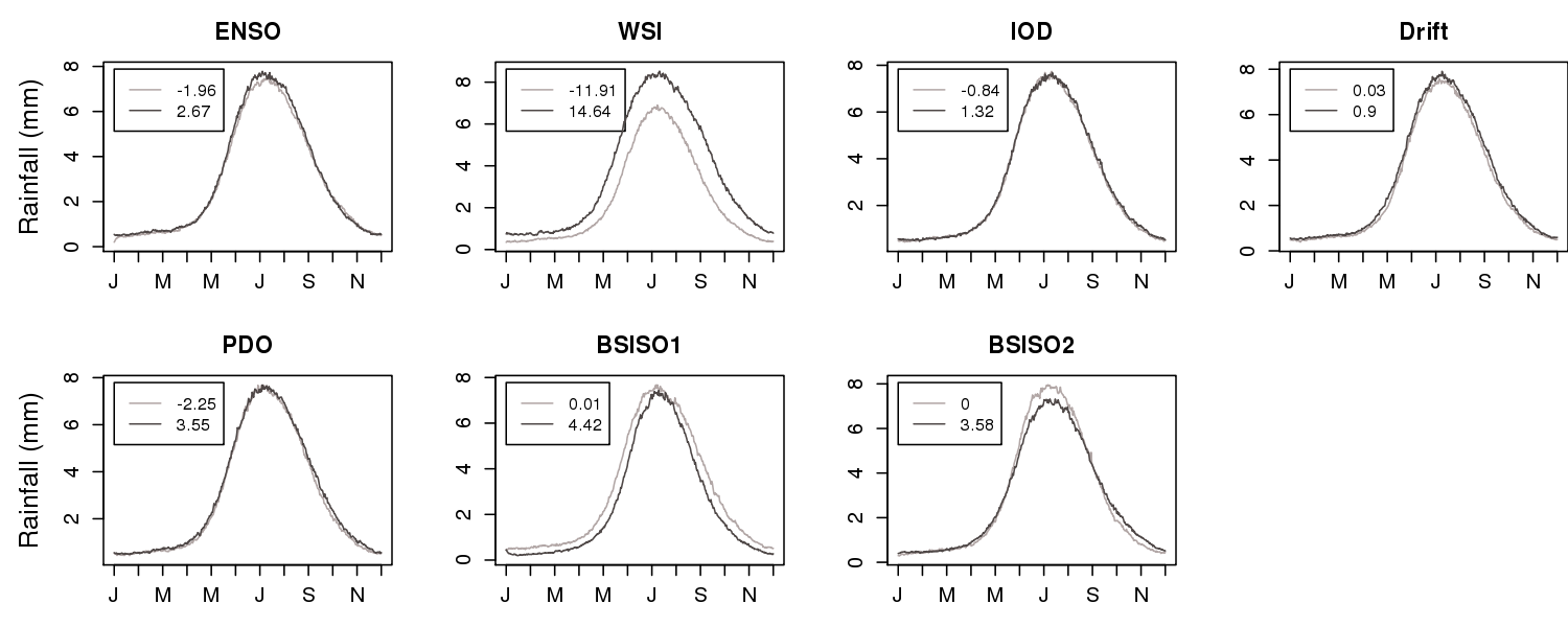
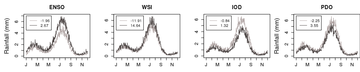
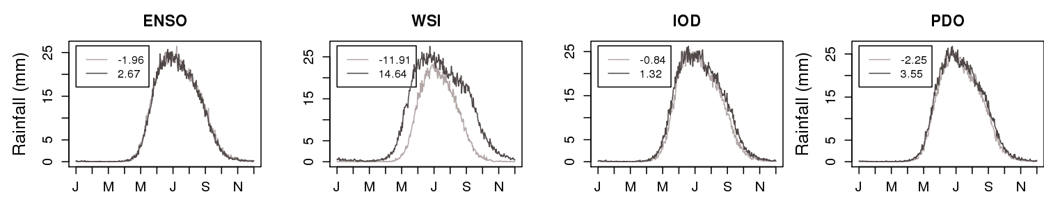
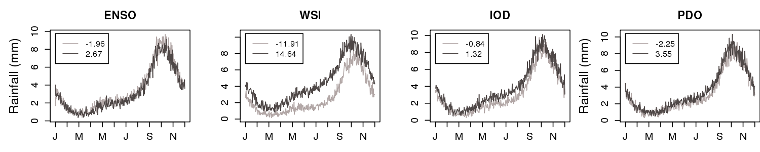
Figure 14 shows similar 1000-chain averaged annual simulations as Figure 13, but for the three selected stations. Years with strong monsoonal wind shear anomalies (WSI) are associated with a much longer summer monsoon rainfall season at the very wet station (station 40) on the west coast, while the impact is on peak rainfall at the “dry” station in NW India (station 3), not duration of the season. The SE India station (station 52), while nominally in the fetch of the NE monsoon that peaks in autumn, nonetheless also feels the summer SW monsoon as well when the monsoonal circulation (given by WSI) is strong, resulting in an extended rainfall season from May–Jan. The indirect climate covariates again have smaller impacts, though they can be quite large at the individual stations. Their impacts are large during summer at station 3 over over inland NW India, although physical interpretation is not straightforward. (See Holsclaw (2017) for additional stations and exogenous variable plots.)
5.4 Spatial Modeling
Finally, we assess the model’s ability to reproduce the observed spatial correlations of the rainfall patterns. Stations that are closer together tend naturally to have more highly correlated measurements, although this can be modulated somewhat by local topography. The two-way station correlations of daily rainfall, for amount and occurrence, range between (0.04,0.41) and (0.04,0.77) respectively. We use two measures of spatial correlation between each pair of stations, the log odds ratio for occurrence and the Spearman’s rank correlation coefficient for rainfall amount. The log odds ratio is calculated for the occurrence (binary classification) as the log of the number of matched days between the two chains divided by the number of differences (Hughes, Guttorp and Charles, 1999).
We compare the observed empirical pairwise correlations to correlations obtained from the 1000 simulated chains of daily rainfall of the same length (each 27 years in length) in Figure 15. The x-axis corresponds to the observed correlations and the y-axis to the simulated correlations. 95% PI bands are included for the simulations. If the model were able to fully reflect the observed spatial correlations then the points in the figure should lie around the diagonal line. The upper panel shows that the spatial correlations tend to be systematically underestimated by the NHMM, which is a known issue in rainfall modeling when assuming that the station variables are conditionally independent given the state variable (Hughes, Guttorp and Charles, 1999; Kirshner, 2010; Germain, 2010). For comparison, the spatial correlations from an equivalent GLM model (with no state structure, which includes the variables, but not variables, as described in Appendix A as Model 3) are shown in the lower panel. The simulated GLM correlations are less accurate than those of the NHMM, indicating that the state variables are contributing to better modeling of spatial dependence. Further improvements could be made by going beyond the conditional independence assumptions within each state, e.g., by using the type of tree-structured station dependence developed in Kirshner, Smyth and Robertson (2004). (See Holsclaw (2017) for similar plots for the three held out years of data.) For more analysis of isotropy and correlation see Holsclaw (2017); these plots show that the NHMM is capturing most of the correlation from the data. Future work could include adding more complex spatial structure to the model but this would have to consider the computational cost as some changes would be prohibitive.


6 Conclusion
We described a Bayesian implementation of the NHMM based on the Polya-Gamma latent variable scheme, allowing for analysis of larger multivariate data sets than possible with prior approaches. The model allows for exogenous variables to influence both the transition probabilities of the hidden states and the emission distributions. The overall approach is flexible in that it can handle non-normally distributed multiple time series of daily data such as rainfall. Sampling is done through a data augmentation approach which removes the need for tuning parameters and makes it nearly automatic.
We illustrated how the framework allows fitting a multivariate NHMM for daily rainfall simulation allowing for incorporation of covariate information of different forms, which is particularly attractive for downscaling of global climate model predictions and projections. In particular we applied the approach to modeling of rainfall data over a large historical collection of daily weather station data across the Indian region. The general distributional properties of Indian rainfall, including seasonality, were shown to be well captured by the model, and spatial correlations between stations adequately captured by the hidden states. The model was shown to be provide particular meteorological insight into the roles of monsoon wind shear strength and intraseasonal wave activity on the seasonality of rainfall in the Indian region. In particular, it enables a novel analysis of rainfall variability integrated from daily-to-seasonal time scales and from local-to-subcontinental spatial scales. This complements the methods traditionally used in monsoon diagnostic and predictability studies that often focus on correlation analysis between variables for a particular spatio-temporal scale, such as the predictability of seasonal averages of all-India rainfall, e.g., (Shukla and Paolino, 1983). More broadly, the Bayesian framework provides uncertainty estimates for all parameters of the model, allowing for assessment of the impact of each exogenous climate variable. The NHMM can be used to generate predictive chains and chains with different levels of the exogenous variables, providing both chains of the hidden states and emission distributions that can be used for model comparison and conditional simulation.
Future work could be aimed at adding a more complex spatial structure between stations to this Polya-Gamma NHMM. Or the conditional independence assumption could be relaxed and subregions could be considered each with their own states. On smaller data sets, some have allowed to be estimated, this could be added to the model. We could also change the modeling assumptions to estimate a coefficient for each of the exogenous variables for each of the states (not the same coefficient for all states). Other NHMM assumptions like having individual coefficients for the transition probabilities could be included instead of just in Equation 1. All changes of this type would include further investigation to model complexity and computational expense as some changes would introduce prohibitive.
Acknowledgment
The rainfall data set was obtained from the Climate Prediction Center, National Centers for Environmental Prediction, National Weather Service, NOAA, U.S. Department of Commerce, from the Research Data Archive at the National Center for Atmospheric Research, Computational and Information Systems Laboratory. http://rda.ucar.edu/datasets/ds512.0. This research was supported by the U.S. Department of Energy, Office of Science, grant DE-SC0006616.
Appendix A: Model Selection
Model Selection Criteria
Model selection has two purposes: to choose the number of states () and select the variables in and . The number of hidden states needs to be determined for the model. More flexible models that allow for change in dimension tend to have complex algorithms that are computationally expensive (i.e., reversible-jump MCMC) (Green, 1995; Robert, Rydén and Titterington, 2000; Meligkotsidou and Dellaportas, 2011). With such large data sets, we can run the NHMM with a few values of (number of hidden states) and use a model selection criterion to choose an optimal number of states. The other model choice is the selection of meaningful exogenous variables. Many exogenous variables can be included in and but some may not be statistically significant.
There are two types of metrics we can consider for the model choice decision: model fit metrics (in-sample) or predictive metrics (out-of-sample). Standard in-sample model fit metrics like Akaike information criterion (AIC), Bayesian information criterion (BIC), and deviance information criterion (DIC) account for the number of parameters used in the model (Akaike, 1974; Schwarz, 1978; Spiegelhalter et al., 2002). We found that in this model because some of the assumptions of the DIC failed to hold, that it tended to choose over-parametrized models. Bayes factors (BF) are not considered because the model has non-informative priors on many of the parameters (Kass and Raftery, 1995; Dempster, 1997). Following the recursive method given in Scott (2002) to calculate the log-likelihood, we report the BIC values which are calculated as negative two times the log-likelihood plus a penalty for the number of parameters times the log number of observations (the parameters are counted: S=63, A=9, B=6, K*(K-1) for , B*(K-1) for , K*S for , A*S for , (K-2)*S for the cutpoints, 2*S*K for , and , , , are latent variables that integrate out and are not counted). The second type of model metric is a predictive measure (out-of-sample) and we consider it the preferable method in this situation. We plan to hold out the last three years of the time series and perform a predictive log score (PLS) (Gneiting and Raftery, 2007; Meligkotsidou and Dellaportas, 2011). After the last observation , there are predictive time steps to the simulated chain ( for three years of predictive chains); the PLS is given by: where is the number of MCMC iterations.
The PLS is calculated for the predictive ability of the model and the BIC is calculated for the model fit. The BIC is calculated from the 27 years model fit (p is the parameter count of the model) and the PLS compares held out three years to predictive conditional chains of three years generated from the model, see Table 2 and Table 1 for results. Table 1 shows several models for comparison with the NHMM and some different configurations of the exogenous variables. Table 2 shows several options of the number of hidden state for the preferred model from Table 1. Overall, the hidden states describe general spatial rainfall patterns, some states capture drier days while others describe wetter weather patterns. This large region may require more states (e.g., seven to twelve) than a more local region, where three to six states might suffice.
Model Selection Results
We run a few baseline models to compare with the NHMM, see Table 1. Model 1 is set up with no states () and no exogenous variables; this spreads rainfall homogeneously throughout the year. Model 2 is a standard weather state NHMM with all inputs (i.e., BSISO1, BSISO2, seasonality (four harmonic components)); the optimal number of states for this model is using BIC. Model 3 treats each station independently () with the GLM linking inputs in (i.e., seasonality (four harmonic components), ENSO,WSI, IOD, Drift, PDO) with the mixing weights (there are no hidden states, thus no inputs). This model is similar to Katz and Parlange (1995); Furrer and Katz (2007); Ailliot and Monbet (2012), where only a single station is modeled. Model 4 uses all inputs of and ; the placement of the inputs into either or was chosen by the climate scientists based on physical properties of the variables (i.e., larger regional variables and shorter time scale in ). Other combinations and inputs were tested but these were the ones that were significant to the model. One of the other models tested was one with only inputs, but it did not perform as well as models including .
Two other models were also considered that had similar (slightly worse) BIC and PLS scores than Model 4. One was a GLM-HMM (Holsclaw et al., 2016; Heaps, Boys and Farrow, 2015) which includes all possible exogenous variables in . This model performed similarly in metrics but has some limitations. Because of climate change, it is of interest to forecast daily rainfall based on evolving variables to modulate the hidden state distributions; the GLM-HMM type of model is stationary and has no mechanism for forecasting climate change like the NHMM. Additionally, another model was considered where all exogenous variables were included in both and . This model performed similarly in metric scores to Model 4 (where variables were limited to being in either or ) but this model had far more parameters and suffered from lack of physical interpretability as the coefficients of and were highly correlated. The most parsimonious and interpretability model is the NHMM with exogenous variables each included once, either in or based on their physical characteristics. Each algorithm was run 2000 iterations with an additional 10% burn in; the samples of the parameters converged quickly to stationarity and the samples mixed well with no thinning (see Holsclaw (2017) for run times and trace plots). The final model was run 10000 iterations with and additional 20% burn in period.
| No. | Model | States | p | BIC | PLS |
|---|---|---|---|---|---|
| 1. | No inputs (no x or w) | 252 | 1565454 | -85.7 | |
| 2. | NHMM for x (no w) | 2079 | 1360954 | -74.2 | |
| 3. | Indep. GLM with w (no x) | 819 | 1406455 | -77.0 | |
| 4. | NHMM with x and w partial | 2283 | 1344892* | -73.6* |
Model 4 had preferable BIC and PLS metrics over all other models. Table 2 shows the the metrics for choosing the number of hidden states () for this model (other models had similar values of ). The table also shows the number of parameters (p); for parsimony we want to choose a model with maximum PLS, minimum BIC, and minimum p (* denotes these values on the Table). denote a model with a single constant state (which is equivalent as having no states ). Table 2 shows that the BIC achieves local minima around seven to ten states. The PLS continues to improve with increased number of states. For parsimony it is sometimes best to choose the number of states where the PLS value is no longer improving as rapidly, this also happens around seven to ten states.
We compare the PLS scores of the NHMM (Model 4) to a baseline model with no states (Model 3). Model 3 fit independent GLM models to each station, whereas Model 4 includes the hidden states and spatial information. Model 3 has a PPL of -77.0 for the baseline model compared to the NHMM with states with a PPL of -73.6. The difference between the two log scores over the three forecast years (predictive conditional chains) is given by , which means the NHMM is 3.1 times better at annual predictive ability. Also, we compare the PLS for Model 4 with states and states: and find only a 1.2 times better annual predictive ability by including the eight additional states.
| K | p | BIC | PLS |
|---|---|---|---|
| 0-1 | 693* | 1405643 | -77.1 |
| 2 | 953 | 1376646 | -75.6 |
| 3 | 1215 | 1366881 | -75.0 |
| 4 | 1479 | 1356233 | -74.4 |
| 5 | 1745 | 1351150 | -74.0 |
| 6 | 2013 | 1346841 | -74.0 |
| 7 | 2283 | 1344892 | -73.6 |
| 8 | 2555 | 1342660 | -73.6 |
| 9 | 2829 | 1342309 | -73.5 |
| 10 | 3105 | 1341327* | -73.3 |
| 11 | 3383 | 1341566 | -73.2 |
| 12 | 3663 | 1341514 | -73.1* |
| 13 | 3945 | 1341798 | -73.2 |
| 14 | 4229 | 1342378 | -73.0* |
| 15 | 4515 | 1342853 | -73.0* |
Appendix B: Climate Variable Details
Six established climate indices related to rainfall in India are: Westerly wind Shear Index (WSI), El Niño/Southern Oscillation (ENSO), Indian Ocean Dipole (IOD), Pacific Decadal Oscillation (PDO), and two components of the boreal summer intraseasonal oscillation (BSISO1 and BSISO2).
- 1
WSI: Year-to-year (interannual) changes in the strength of the summer monsoon winds are closely linked with monsoon rainfall variations, and we use the Westerly Shear Index (WSI), as defined in Wang and Fan (1999) as WSI1, to represent these. The WSI is defined by the vertical shear of the zonal wind (u850 −- u200 ) averaged over the box (5N–20N, 40E–80E), and was used in an NHMM for Indian rainfall by Greene et al. (2011). We use monthly-averaged values, with the mean seasonal cycle subtracted, so as to focus on interannual variations in the monsoon circulation.
- 2-3
ENSO and IOD: ENSO and IOD indices were computed from the NOAA Extended Reconstructed Sea Surface Temperature Dataset, version 3b Smith et al. (2008), via the IRI Data Library (http://iri.columbia.edu). The El Niño/Southern Oscillation (ENSO) and Indian Ocean Dipole (IOD) are known influences on rainfall on interannual time scales (Gadgil, 2003). Monthly sea surface temperature (SST) in the Nino3.4 region (150W-90W, 5N-5S) are used to define the ENSO index the monsoon tends to be stronger during the La Nina phase, when this ENSO index is negative (Gadgil, 2003). The IOD index is defined by the difference in monthly SST anomalies in the western (50E–70E, 10N–10S) and eastern (90E–110E and 0S–10S) equatorial Indian Ocean; the monsoon tends to be stronger when IOD is positive (Gadgil, 2003).
- 4
PDO: While the Pacific Decadal Oscillation (PDO) has a less well understood impact (Joseph et al., 2013). The PDO index is defined by Zhang, Wallace and Battisti (1997) to be the leading PC of monthly SST anomalies in the North Pacific Ocean, poleward of 20N. The monthly mean global average SST anomalies are removed to separate this pattern of variability from any “global warming” signal that may be present in the data. This data set set is from University of Washington (http://research.jisao.washington.edu/data_sets/pdo/)
- 5-6
BSISO 1 and 2: On sub-seasonal time scales Indian monsoon rainfall is impacted by the boreal summer intraseasonal oscillation (BSISO), data obtained from the APEC Climate Center (APCC, http://www.apcc21.org) (Lau and Chan, 1986; Yoo, Robertson and Kang, 2010), for which we use the two indices BSISO 1 and 2 defined by (Lee et al., 2013).
The cross-correlations between these daily series are given in Table 3 and are relatively low. Monsoon circulation anomalies (WSI) are quite strongly related to ENSO and PDO (r = -0.51 and 0.41 resp.), less strongly with IOD (r = 0.28), but not to the BSISO.
| ENSO | WSI | IOD | PDO | BSISO1 | BSISO2 | |
|---|---|---|---|---|---|---|
| ENSO | — | -0.51 | 0.28 | 0.41 | -0.01 | 0.02 |
| WSI | — | -0.19 | -0.25 | -0.01 | -0.04 | |
| IOD | — | 0.09 | -0.03 | -0.02 | ||
| PDO | — | -0.08 | 0.01 | |||
| BSISO1 | — | 0.07 | ||||
| BSISO2 | — |
References
- Ailliot and Monbet (2012) [author] Ailliot, P.P. and Monbet, V.V. (2012). Markov-switching autoregressive models for wind time series. Environ. Model. Softw. 30 92-101.
- Ailliot et al. (2015) [author] Ailliot, P.P., Allard, D.D., Monbet, V.V. and Naveau, P.P. (2015). Stochastic weather generators: an overview of weather type models. J. Soc. Fr. Statistique 156 101–113.
- Aitchison and Bennett (1970) [author] Aitchison, J.J. and Bennett, J.J. (1970). Polychotomous quantal response by maximum indicant. Biometrika 57 253–262.
- Akaike (1974) [author] Akaike, H.H. (1974). A new look at the statistical model identification. IEEE Trans. Autom. Control 19 716–723.
- Albert and Chib (1993) [author] Albert, J. H.J. H. and Chib, S.S. (1993). Bayesian analysis of binary and polychotomous response data. J. Amer. Statist. Assoc. 88 669-679.
- Bellone, Hughes and Guttorp (2000) [author] Bellone, EnricaE., Hughes, James P.J. P. and Guttorp, PeterP. (2000). A hidden Markov model for downscaling synoptic atmospheric patterns to precipitation amounts. Climate Res. 15 1–12.
- Berrocal, Gelfand and Holland (2010) [author] Berrocal, V. J.V. J., Gelfand, A. E.A. E. and Holland, D. M.D. M. (2010). A bivariate space–time downscaler under space and time misalignment. Ann. Appl. Stat. 4 1942–1975.
- Carey-Smith, Sansom and Thomson (2014) [author] Carey-Smith, T.T., Sansom, J.J. and Thomson, P.P. (2014). A hidden seasonal switching model for multisite daily rainfall. Water Resour. Res. 50 257-272.
- Challinor et al. (2009) [author] Challinor, Andrew JA. J., Ewert, FrankF., Arnold, SteveS., Simelton, ElisabethE. and Fraser, EvanE. (2009). Crops and climate change: progress, trends, and challenges in simulating impacts and informing adaptation. J. Exp. Bot. 60 2775–2789.
- Charles, Bates and Hughes (1999) [author] Charles, Stephen P.S. P., Bates, Bryson C.B. C. and Hughes, James P.J. P. (1999). A spatiotemporal model for downscaling precipitation occurrence and amounts. J. Geophys. Res. 104 31657–31669.
- Charles et al. (2004) [author] Charles, Stephen PS. P., Bates, Bryson CB. C., Smith, Ian NI. N. and Hughes, James PJ. P. (2004). Statistical downscaling of daily precipitation from observed and modelled atmospheric fields. Hydrol. Process. 18 1373–1394.
- Chib and Greenburg (1998) [author] Chib, S.S. and Greenburg, E.E. (1998). Analysis of multivariate probit models. Biometrika 85 347–361.
- Cox (1971) [author] Cox, D. R.D. R. (1971). The Analysis of Binary Data. Methuen, London.
- Dempster (1997) [author] Dempster, A. P.A. P. (1997). The direct use of likelihood for significance testing. Statist. Comput. 7 247–252.
- Dempster, Laird and Rubin (1977) [author] Dempster, A. P.A. P., Laird, N. M.N. M. and Rubin, D. R.D. R. (1977). Maximum likelihood from incomplete data via the EM algorithm. J. R. Stat. Soc. Series B Stat. Methodol. 39 1–38.
- Diebold and Lee (1994) Diebold, F. X. and Lee, J. H. (1994). Regime switching with time-varying transition probabilities. In Nonstationary Time Series Analysis and Cointegrations (C. W. J. Granger and G. Mixon, eds.) 283–302. Oxford University Press.
- Filardo and Gordon (1998) [author] Filardo, Andrew JA. J. and Gordon, Stephen FS. F. (1998). Business cycle durations. J. Econometrics 85 99–123.
- Forney (1978) [author] Forney, G. D.G. D. (1978). The Viterbi algorithm. Proc. IEEE 61 268–278.
- Frühwirth-Schnatter (2006) [author] Frühwirth-Schnatter, SylviaS. (2006). Finite Mixture and Markov Switching Models. Springer Science & Business Media.
- Frühwirth-Schnatter (2008) [author] Frühwirth-Schnatter, S.S. (2008). Data augmentation and dynamic linear models. J. Time Ser. Anal. 15 183–202.
- Frühwirthh-Schnatter and Frühwirth (2007) [author] Frühwirthh-Schnatter, S.S. and Frühwirth, R.R. (2007). Auxiliary mixture sampling with applications to logistic models. Comput. Stat. Data Anal. 51 3509-28.
- Fuentes and Raftery (2005) [author] Fuentes, M.M. and Raftery, A. E.A. E. (2005). Model evaluation and spatial interpolation by Bayesian combination of observations with outputs from numerical models. Biometrics 61 36–45.
- Furrer and Katz (2007) [author] Furrer, E. M.E. M. and Katz, R. W.R. W. (2007). Generalized linear modeling approach to stochastic weather generators. Climate Res. 34 129–144.
- Gadgil (2003) [author] Gadgil, SulochanaS. (2003). The Indian monsoon and its variability. Ann. Rev. Earth Planet. Sci. 31 429-467. 10.1146/annurev.earth.31.100901.141251
- Germain (2010) [author] Germain, S.S. (2010). Bayesian spatio-temporal modelling of rainfall through non-homogenous hidden Markov models PhD thesis, Newcastle University, Newcastle, UK.
- Gershunov, Schneider and Barnet (2001) [author] Gershunov, AlexanderA., Schneider, NiklasN. and Barnet, TimT. (2001). Low-frequency modulation of the ENSO-Indian monsoon rainfall relationship: Signal or noise? J. Climate 14 2486–2492.
- Ghil and Robertson (2002) [author] Ghil, M.M. and Robertson, A. W.A. W. (2002). “Waves” vs. “particles” in the atmosphere’s phase space: A pathway to long-range forecasting? Proc. Natl. Acad. Sci. USA 99 (Suppl. 1) 2493–2500.
- Gneiting and Raftery (2007) [author] Gneiting, TilmannT. and Raftery, Adrian EA. E. (2007). Strictly proper scoring rules, prediction, and estimation. J. Amer. Statist. Assoc. 102 359–378.
- Green (1995) [author] Green, Peter J.P. J. (1995). Reversible jump Markov chain Monte Carlo computation and Bayesian model determination. Biometrika 82 711–732.
- Greene, Robertson and Kirshner (2008) [author] Greene, A. M.A. M., Robertson, A. W.A. W. and Kirshner, S.S. (2008). Analysis of Indian monsoon daily rainfall on subseasonal to multidecadal time-scales using a hidden Markov model. Q.J.R. Meteorol. Soc. 134 875–887.
- Greene et al. (2011) [author] Greene, A. M.A. M., Robertson, A. W.A. W., Smyth, P.P. and Triglia, S.S. (2011). Downscaling projectios of the Indian monsoon rainfall using a non-homogeneous hidden Markov model. Q.J.R. Meteorol. Soc. 137 347–359.
- Hansen et al. (2006) [author] Hansen, James W.J. W., Challinor, AndrewA., Ines, AmorA., Wheeler, TimT. and Moron, VincentV. (2006). Translating climate forecasts into agricultural terms: advances and challenges. Climate Res. 33 27–41.
- Hay (1991) [author] Hay, L. E. et alL. E. et al. (1991). Simulation of precipitation by weather type analysis. Water Resour. Res. 27 493–501.
- Heaps, Boys and Farrow (2015) [author] Heaps, S. E.S. E., Boys, R. J.R. J. and Farrow, M.M. (2015). Bayesian modelling of rainfall data by using non-homogeneous hidden Markov models and latent Gaussian variables. J. R. Stat. Soc. Series C App. Stat. 64 543-568.
- Holmes and Held (2006a) [author] Holmes, C.C. and Held, L.L. (2006a). Bayesian auxiliary variable models for binary and multinomial regression. Bayesian Anal. 1 145–168.
- Holmes and Held (2006b) [author] Holmes, C.C. and Held, L.L. (2006b). Response to van der Lans. Bayesian Anal. 6 357–358.
- Holsclaw (2017) [author] Holsclaw, T. et alT. et al. (2017). Supplement to “Bayesian non-homogeneous Markov models via Polya-Gamma data augmentation with applications to rainfall modeling”.
- Holsclaw et al. (2016) [author] Holsclaw, TracyT., Greene, Arthur MA. M., Robertson, Andrew WA. W. and Smyth, PadhraicP. (2016). A Bayesian hidden Markov model of daily precipitation over South and East Asia. J. Hydrometeorol. 17.
- Hooten and Wikle (2010) [author] Hooten, M. B.M. B. and Wikle, C. K.C. K. (2010). Statistical agent-based models for discrete spatio-temporal systems. J. Amer. Statist. Assoc. 105 236–248.
- Hughes and Guttorp (1994) [author] Hughes, J. P.J. P. and Guttorp, P.P. (1994). A class of stochastic models for relating synoptic atmospheric patterns to regional hydrologic phenomena. Water Resour. Res. 30 1535–1546.
- Hughes, Guttorp and Charles (1999) [author] Hughes, James PJ. P., Guttorp, PeterP. and Charles, Stephen PS. P. (1999). A non-homogeneous hidden Markov model for precipitation occurrence. J. R. Stat. Soc. Series C App. Stat. 48 15–30.
- Imai and van Dyk (2005) [author] Imai, K.K. and van Dyk, D. A.D. A. (2005). MNP: R package for fitting the multinomial probit model. J. of Stat. Softw. 14 1–32.
- Immerzeel, van Beek and Bierkens (2010) [author] Immerzeel, Walter W.W. W., van Beek, Ludovicus P. H.L. P. H. and Bierkens, Marc F. P.M. F. P. (2010). Climate change will affect the Asian water towers. Science 328 1382–1385.
- Jasra, Holmes and Stephens (2005) [author] Jasra, A.A., Holmes, C. C.C. C. and Stephens, D. A.D. A. (2005). Markov chain Monte Carlo and the label switching problem in Bayesian mixture modelling. J. Stat. Plan. Inference. 20 2305-2315.
- Johndrow, Lum and Dunson (2013) [author] Johndrow, J. E.J. E., Lum, K.K. and Dunson, D.D. (2013). Diagonal orthant multinomial probit models. AISTATS and JMLR(31) 29–38.
- Joseph et al. (2013) [author] Joseph, Porathur VareedP. V., Gokulapalan, BinduB., Nair, ArchanaA. and Wilson, Shinu SheelaS. S. (2013). Variability of summer monsoon rainfall in India on inter-annual and decadal time scales. Atmos. Oceanic Sci. Lett. 6 398–403. 10.3878/j.issn.1674-2834.13.0044
- Jurafsky and Martin (2014) [author] Jurafsky, D.D. and Martin, J. H.J. H. (2014). Speech and Language Processing. Prentice Hall.
- Kass and Raftery (1995) [author] Kass, R. E.R. E. and Raftery, A. E.A. E. (1995). Bayes factors. J. Amer. Statist. Assoc. 90 773–795.
- Katz and Parlange (1995) [author] Katz, R.R. and Parlange, M.M. (1995). Generalization of chain-dependent processes: Application to hourly precipitation. Water Resour. Res. 31 1331–1341.
- Kim, Piger and Startz (2008) [author] Kim, Chang-JinC.-J., Piger, JeremyJ. and Startz, RichardR. (2008). Estimation of Markov regime-switching regression models with endogenous switching. J. Econometrics 143 263–273.
- Kirshner (2010) [author] Kirshner, S.S. (2010). Modeling of multivariate time series using hidden Markov models PhD thesis, University of California, Irvine.
- Kirshner, Smyth and Robertson (2004) Kirshner, S., Smyth, P. and Robertson, A. W. (2004). Conditional Chow-Liu tree structures for modeling discrete-valued vector time series. In Proc. 20th Conf. UAI 317–324.
- Lau and Chan (1986) [author] Lau, Ka-MingK.-M. and Chan, P. H.P. H. (1986). Aspects of the 40–50 day oscillation during the northern summer as inferred from outgoing longwave radiation. Mon. Wea. Rev. 114 1354–1367.
- Lee et al. (2013) [author] Lee, J. Y.J. Y., Wang, B.B., Wheeler, M. C.M. C., Fu, X.X., Waliser, D. E.D. E. and Kang, I. S.I. S. (2013). Real-time multivariate indices for the boreal summer intraseasonal oscillation over the Asian summer monsoon region. Clim. Dyn. 40 493–509. 10.1007/s00382-012-1544-4
- MacDonald and Zucchini (1997) [author] MacDonald, I. L.I. L. and Zucchini, W.W. (1997). Hidden Markov and other models for discrete-valued time series. Number 70 in Monographs on Statistics and Applied Probability. Chapman and Hall, New York.
- Mamon and Elliott (2007) [author] Mamon, Rogemar SR. S. and Elliott, Robert JamesR. J. (2007). Hidden Markov Models in Finance. Springer.
- Maraun et al. (2010) [author] Maraun, DouglasD., Wetterhall, FF., Ireson, AMA., Chandler, RER., Kendon, EJE., Widmann, MM., Brienen, SS., Rust, HWH., Sauter, TT., Themeßl, MM. et al. (2010). Precipitation downscaling under climate change: Recent developments to bridge the gap between dynamical models and the end user. Rev. Geophys. 48 1–34.
- McCullagh and Nelder (1989) [author] McCullagh, P.P. and Nelder, J.J. (1989). Generalized Linear Models. Chapman and Hall, New York.
- McCulloch, Polson and Rossi (2000) [author] McCulloch, R.R., Polson, N. G.N. G. and Rossi, P. E.P. E. (2000). A Bayesian analysis of the multinomial probit model with fully identified parameters. J. Econometrics 99 173–193.
- Meligkotsidou and Dellaportas (2011) [author] Meligkotsidou, LoukiaL. and Dellaportas, PetrosP. (2011). Forecasting with non-homogeneous hidden Markov models. Statistics and Computing 21 439–449.
- Moron, Robertson and Ghil (2012) [author] Moron, V.V., Robertson, A. W.A. W. and Ghil, M.M. (2012). Impact of the modulated annual cycle and intraseasonal oscillation on daily-to-interannual rainfall variability across monsoonal India. Climate Dyn. 38 2409–2435. 10.1007/s00382-011-1253-4
- Neal (1997) [author] Neal, R. M.R. M. (1997). Monte Carlo implementation of Gaussian process models for Bayesian regression and classification. Technical Report No. 9702, Department of Statistics, University of Toronto 1–24.
- O’Brien and Dunson (2004) [author] O’Brien, S. M.S. M. and Dunson, D. B.D. B. (2004). Bayesian multivariate logistic regression. Biometrics 60 739–746.
- Paap and Frances (2000) [author] Paap, R.R. and Frances, P. H.P. H. (2000). A dynamic multinomial probit model for brand choices with different short–run effects of marketing mix variables. J. of Appl. Econometrics 15 717–744.
- Paroli and Spezia (2008) [author] Paroli, R.R. and Spezia, L.L. (2008). Bayesian inference in non-homogeneous Markov mixtures of periodic autoregressions with state-dependent exogenous variables. Comput. Stat. Data Anal. 52 2311–2330.
- Patterson et al. (2016) [author] Patterson, T. A.T. A., Parton, A.A., Langrock, R.R., Blackwell, P. G.P. G., Thomas, L.L. and King, R.R. (2016). Statistical modelling of animal movement: A myopic review and a discussion of good practice. http://arxiv.org/abs/0901.4804.
- Piani et al. (2010) [author] Piani, CC., Weedon, GPG., Best, MM., Gomes, SMS., Viterbo, PP., Hagemann, SS. and Haerter, JOJ. (2010). Statistical bias correction of global simulated daily precipitation and temperature for the application of hydrological models. J. Hydrol. 395 199–215.
- Polson, Scott and Windle (2013) [author] Polson, N. G.N. G., Scott, J. G.J. G. and Windle, J.J. (2013). Bayesian inference for logistic models using Polya-Gamma latent variables. J. Amer. Statist. Assoc. 108 1339–1349.
- Rajagopalan, Lall and Tarboton (1996) [author] Rajagopalan, B.B., Lall, U.U. and Tarboton, D. G.D. G. (1996). Nonhomogeneous Markov model for daily precipitation. J. Hydrol. Eng. 1 33-40.
- Raphael (1999) [author] Raphael, ChristopherC. (1999). Automatic segmentation of acoustic musical signals using hidden Markov models. IEEE Trans. Pattern Anal. Mach. Intell. 21 360–370.
- Riihimaki, Jylanki and Vehtari (2013) [author] Riihimaki, J.J., Jylanki, P.P. and Vehtari, A.A. (2013). Nested expectation propagation for Gaussian process classification with a multinomial probit likelihood. J. Mach. Learn. Res. 14 75–109.
- Robert, Rydén and Titterington (2000) [author] Robert, C. P.C. P., Rydén, T.T. and Titterington, D. M.D. M. (2000). Bayesian inference in hidden Markov models through the reversible jump Markov chain Monte Carlo method. J. R. Stat. Soc. Series B Stat. Methodol. 62 57–75.
- Robertson (2009) [author] Robertson, A. W.A. W. (2009). Seasonal predictability of daily rainfall statistics over Indramayu district, Indonesia. Int. J. Climatol. 29 1449–1462.
- Rydén (2008) [author] Rydén, T.T. (2008). EM versus Markov chain Monte Carlo for estimation of hidden Markov models: A computational perspective. Bayesian Anal. 3 659–688.
- Schwarz (1978) [author] Schwarz, Gideon E.G. E. (1978). Estimating the dimension of a model. Ann. Stat. 6 461–464.
- Scott (2002) [author] Scott, S. L.S. L. (2002). Bayesian methods for hidden Markov models: Recursive computing in the 21st century. J. Amer. Statist. Assoc. 97 337–351.
- Scott (2011) [author] Scott, S. L.S. L. (2011). Data augmentation, frequentist estimation, and the Bayesian analysis of multinomial logit models. Stat. Papers 52 87–109.
- Shukla and Paolino (1983) [author] Shukla, J.J. and Paolino, D. A.D. A. (1983). The southern oscillation and long-range forecasting of the summer monsoon rainfall over India. Mon. Wea. Rev. 111 1830-1837.
- Siepel and Haussler (2004) [author] Siepel, AdamA. and Haussler, DavidD. (2004). Combining phylogenetic and hidden Markov models in biosequence analysis. J. Comput. Bio. 11 413–428.
- Smith et al. (2008) [author] Smith, T. M.T. M., Reynolds, R. W.R. W., Peterson, Thomas C.T. C. and Lawrimore, JayJ. (2008). Improvements to NOAA’s historical merged land-ocean surface temperature analysis (1880-2006). J. Climate 21 2283–2296.
- Spezia (2009) [author] Spezia, L.L. (2009). Reversible jump and the label switching problem in hidden Markov models. Stat. Sci. 139 50–67.
- Spezia et al. (2014) [author] Spezia, LL., Cooksley, SLS., Brewer, MJM., Donnelly, DD. and Tree, AA. (2014). Modelling species abundance in a river by Negative Binomial hidden Markov models. Comput. Stat. Data Anal. 71 599–614.
- Spiegelhalter et al. (2002) [author] Spiegelhalter, David J.D. J., Best, Nicola G.N. G., Carlin, Bradley P.B. P. and van der Linde, AngelikaA. (2002). Bayesian measure of model complexity and fit. J. R. Stat. Soc. Series B Stat. Methodol. 64 583–639.
- Stern and Coe (1984) [author] Stern, R. D.R. D. and Coe, R.R. (1984). A model fitting analysis of daily rainfall data. J. R. Statist. Soc. A 147 1–34.
- Vermeulen et al. (2013) [author] Vermeulen, Sonja JS. J., Challinor, Andrew JA. J., Thornton, Philip KP. K., Campbell, Bruce MB. M., Eriyagama, NishadiN., Vervoort, Joost MJ. M., Kinyangi, JamesJ., Jarvis, AndyA., Läderach, PeterP., Ramirez-Villegas, JulianJ. et al. (2013). Addressing uncertainty in adaptation planning for agriculture. Proc. Natl. Acad. Sci. 110 8357–8362.
- Wang and Fan (1999) [author] Wang, BinB. and Fan, ZhenZ. (1999). Choice of south Asian summer monsoon indices. Bull. Am. Met. Soc. 80 629–638.
- Wilks (1998) [author] Wilks, D. S.D. S. (1998). Multisite generalization of a daily stochastic precipitation generation model. J. Hydrol. 210 178–191.
- Wilks (1999a) [author] Wilks, D. S.D. S. (1999a). Interannual variability and extreme-value characteristics of several stochastic daily precipitation models. Agric. Forest Meteor. 93 153–170.
- Wilks (1999b) [author] Wilks, D. S.D. S. (1999b). Multisite downscaling of daily precipitation with a stochastic weather generator. Clim. Res. 11 125–136.
- Wilks and Wilby (1999) [author] Wilks, D. S.D. S. and Wilby, R. L.R. L. (1999). The weather generation game: a review of stochastic weather models. Prog. in Phys. Geogr. 23 329–357.
- Woolhiser and Roldan (1982) [author] Woolhiser, D. A.D. A. and Roldan, J.J. (1982). Stochastic daily precipitation models 2. A comparison of distributions of amounts. Water Resour. Res. 18 1461–1468.
- Yoo, Robertson and Kang (2010) [author] Yoo, Jin HoJ. H., Robertson, Andrew W.A. W. and Kang, In-SikI.-S. (2010). Analysis of intraseasonal and interannual variability of the Asian summer monsoon using a hidden Markov model. J. Climate 23 5498–5516. 10.1175/2010JCLI3473.1
- Zhang, Boscardin and Belin (2008) [author] Zhang, X.X., Boscardin, W. J.W. J. and Belin, T. R.T. R. (2008). Bayesian analysis of multivariate nominal measures using multivariate multinomial probit models. Comput. Stat. Data Anal. 52 3697–3708.
- Zhang, Wallace and Battisti (1997) [author] Zhang, Y.Y., Wallace, J. M.J. M. and Battisti, D. S.D. S. (1997). ENSO-like interdecadal variability: 1900-93. J. Climate 10 1004–1020.
- Zucchini and Guttorp (1991) [author] Zucchini, W.W. and Guttorp, P.P. (1991). A hidden Markov model for space-time precipitation. Water Resour. Res. 27 1917-1923.
- Zucchini, MacDonald and Langrock (2016) [author] Zucchini, W.W., MacDonald, I.I. and Langrock, R.R. (2016). Hidden Markov Models for Time Series: An Introduction using R. Chapman and Hall, Boca Raton.