跳到论文正文
W Papers独立论文阅读器 arXiv:1701.02818 论文正文 计算阅读时间 · 0%
引用这篇论文根据当前论文元数据生成,正式投稿前建议核对。


License: arXiv.org perpetual non-exclusive license
arXiv:1701.02818v5 [math.NA] 30 Jun 2018

Numerical analysis of nonlocal fracture models in Hölder spaceThanks: Published on SIAM Journal on Numerical Analysis on April 10, 2018.

Prashant K. Jha ††thanks: Department of Mathematics, Louisiana State University, Baton Rouge, LA (). Email: prashant.j16o@gmail.com    Robert Lipton ††thanks: Department of Mathematics, Louisiana State University, Baton Rouge, LA (). Email: lipton@math.lsu.edu
Abstract

In this work, we calculate the convergence rate of the finite difference approximation for a class of nonlocal fracture models. We consider two point force interactions characterized by a double well potential. We show the existence of a evolving displacement field in Hölder space with Hölder exponent γ∈(0,1]\gamma\in(0,1]. The rate of convergence of the finite difference approximation depends on the factor Cs​hγ/ϵ2C_{s}h^{\gamma}/\epsilon^{2} where ϵ\epsilon gives the length scale of nonlocal interaction, hh is the discretization length and CsC_{s} is the maximum of Hölder norm of the solution and its second derivatives during the evolution. It is shown that the rate of convergence holds for both the forward Euler scheme as well as general single step implicit schemes. A stability result is established for the semi-discrete approximation. The Hölder continuous evolutions are seen to converge to a brittle fracture evolution in the limit of vanishing nonlocality.

keywords
Nonlocal fracture models, peridynamics, cohesive dynamics, numerical analysis, finite difference approximation
Funding.
This material is based upon work supported by the U. S. Army Research Laboratory and the U. S. Army Research Office under contract/grant number W911NF1610456.
††runningheads: Numerical analysis of nonlocal fracture models in Hölder space / Prashant K. Jha and Robert Lipton
AMS
34A34, 34B10, 74H55, 74S20

1 Introduction

Nonlocal formulations have been proposed to describe the evolution of deformations which exhibit loss of differentiability and continuity, see [28] and [31]. These models are commonly referred to as peridynamic models. The main idea is to define the strain in terms of displacement differences and allow nonlocal interactions between material points. This generalization of strain allows for the participation of a larger class of deformations in the dynamics. Numerical simulations based on peridynamic modeling exhibit formation and evolution of sharp interfaces associated with phase transformation and fracture [9], [32], [27], [16], [1], [11], [24], [6], [20], [30], [34], [17]. A recent summary of the state of the art can be found in [14].

In this work, we provide a numerical analysis for the class of nonlocal models introduced in [22] and [23]. These models are defined by a double well two point potential. Here one potential well is centered at zero and associated with elastic response while the other well is at infinity and associated with surface energy. The rational for studying these models is that they are shown to be well posed over the class of square integrable non-smooth displacements and, in the limit of vanishing non-locality, their dynamics recover features associated with sharp fracture propagation see, [22] and [23]. The numerical simulation of prototypical fracture problems using this model is carried out in [24]. In order to develop an L2L^{2} approximation theory, we show the nonlocal evolution is well posed over a more regular space of functions. To include displacement fields which have no well-defined derivatives, we consider displacement fields in the Hölder space C0,γC^{0,\gamma} with Hölder exponent γ\gamma taking any value in (0,1](0,1]. We show that a unique evolution exists in C0,γC^{0,\gamma} for C0,γC^{0,\gamma} initial data and body force. The semi-discrete approximation to the Hölder continuous evolution is considered and it is shown that at any time its energy is bounded by the initial energy and the work done by the body force. We develop an approximation theory for the forward Euler scheme and show that these ideas can be easily extended to the backward Euler scheme as well other implicit one step time discretization schemes. It is found that the discrete approximation converges to the exact solution in the L2L^{2} norm uniformly over finite time intervals with the rate of convergence proportional to (Ct​Δ​t+Cs​hγ/ϵ2)(C_{t}\Delta t+C_{s}h^{\gamma}/\epsilon^{2}), where Δ​t\Delta t is the size of time step, hh is the size of spatial mesh discretization, and ϵ\epsilon is the length scale of nonlocal interaction relative to the size of the domain. The constant CtC_{t} depends on the L2L^{2} norm of the time derivatives of the solution, CsC_{s} depends on the Hölder norm of the solution and the Lipschitz constant of peridynamic force. We point out that the constants appearing in the convergence estimates with respect to hh can be dependent on the horizon and be large when ϵ\epsilon is small. This is discussed in section 3 and an example is provided in section 6. These results show that while errors can grow with each time step they can be controlled over finite times tt by suitable spatial temporal mesh refinement. We then apply the methods developed in [22] and [23], to show that in the limit ϵ→0\epsilon\rightarrow 0, the Hölder continuous evolutions converge to a limiting sharp fracture evolution with bounded Griffiths fracture energy. Here the limit evolution is differentiable off the crack set and satisfies the linear elastic wave equation.

In the language of nonlocal operators, the integral kernel associated with the nonlocal model studied here is Lipschitz continuous guaranteeing global stability of the finite difference approximation. This is in contrast to PDE based evolutions where stability can be conditional. In addition we examine local stability. Unfortunately the problem is nonlinear so we don’t establish CFL conditions but instead identify a mode of dynamic instability that can arise during the evolution. This type of instability is due to a radial perturbation of the solution and causes error to grow with each time step for the Euler scheme. For implicit schemes this perturbation can become unstable in parts of the computational domain where there is material softening, see subsection 3.4. Of course stability conditions like the CFL conditions for linear nonlocal equations are of importance for guidance in implementations. In the case of d=1d=1, a CFL type condition is obtained for the finite difference and finite element approximation of the linear peridynamic equation, see [18]. Recent work develops a new simple CFL condition for one dimensional linearized peridynamics in the absence of body forces [15]. Related analysis for the linear peridynamic equation in one dimension is taken up in [35] and [7]. The recent and related work [12] and [19] addresses numerical approximation for problems of nonlocal diffusion.

There is now a large body of contemporary work addressing the numerical approximation of singular kernels with application to nonlocal diffusion, advection, and mechanics. Numerical formulations and convergence theory for nonlocal pp-Laplacian formulations are developed in [13], [26]. Numerical analysis of nonlocal steady state diffusion is presented in [33] and [25], and [8]. The use of fractional Sobolev spaces for nonlocal problems is investigated and developed in [12]. Quadrature approximations and stability conditions for linear peridynamics are analyzed in [35] and [29]. The interplay between nonlocal interaction length and grid refinement for linear peridynamic models is presented in [7]. Analysis of adaptive refinement and domain decomposition for linearized peridynamics are provided in [3], [21], and [2]. This list is by no means complete and the literature on numerical methods and analysis continues to grow.

The paper is organized as follows. In section 2, we describe the nonlocal model. In subsection 2.2, we state theorems which show Lipschitz continuity of the nonlocal force (Proposition 1) and the existence and uniqueness of an evolution over any finite time interval (Theorem 2). In section 3, we compute the convergence rate of the forward Euler scheme as well as implicit one step methods. We identify stability of the semi-discrete approximation with respect to the energy in subsection 3.3. In subsection 3.4, we identify local instabilities in the fully discrete evolution caused by suitable radial perturbations of the solution. In section 4, we give the proof of Proposition 1, Theorem 6, and Theorem 2. The convergence of Hölder continuous evolutions to sharp fracture evolutions as ϵ→0\epsilon\rightarrow 0 is shown in section 5. In section 6 we present an example showing the effect of the constants CtC_{t} and CsC_{s} on the convergence rate and summarize our results.

2 Double well potential and existence of a solution

In this section, we present the nonlinear nonlocal model. Let D⊂ℝdD\subset\mathbb{R}^{d}, d=2,3d=2,3 be the material domain with characteristic length-scale of unity. Let ϵ∈(0,1]\epsilon\in(0,1] be the size of horizon across which nonlocal interaction between points takes place. The material point 𝒙∈D\boldsymbol{x}\in D interacts nonlocally with all material points inside a horizon of length ϵ\epsilon. Let Hϵ​(𝒙)H_{\epsilon}(\boldsymbol{x}) be the ball of radius ϵ\epsilon centered at 𝒙\boldsymbol{x} containing all points 𝒚\boldsymbol{y} that interact with 𝒙\boldsymbol{x}. After deformation the material point 𝒙\boldsymbol{x} assumes position 𝒛=𝒙+𝒖⁡(𝒙)\boldsymbol{z}=\boldsymbol{x}+\boldsymbol{u}(\boldsymbol{x}). In this treatment we assume infinitesimal displacements and the strain is written in terms of the displacement 𝒖\boldsymbol{u} as

S=S⁡(𝒚,𝒙,𝒖)\displaystyle S=S(\boldsymbol{y},\boldsymbol{x};\boldsymbol{u}) :=𝒖⁡(𝒚)−𝒖⁡(𝒙)|𝒚−𝒙|⋅𝒚−𝒙|𝒚−𝒙|.\displaystyle:=\dfrac{\boldsymbol{u}(\boldsymbol{y})-\boldsymbol{u}(\boldsymbol{x})}{\left\lvert\boldsymbol{y}-\boldsymbol{x}\right\rvert}\cdot\dfrac{\boldsymbol{y}-\boldsymbol{x}}{\left\lvert\boldsymbol{y}-\boldsymbol{x}\right\rvert}.

Let Wϵ​(S,𝒚−𝒙)W^{\epsilon}(S,\boldsymbol{y}-\boldsymbol{x}) be the nonlocal potential density per unit length between material point 𝒚\boldsymbol{y} and 𝒙\boldsymbol{x}. The energy density at 𝒙\boldsymbol{x} is given by

𝑾ϵ​(S,𝒙)=1ϵd​ωd​∫Hϵ​(𝒙)|𝒚−𝒙|​Wϵ​(S,𝒚−𝒙)​𝑑𝒚,\displaystyle\boldsymbol{W}^{\epsilon}(S,\boldsymbol{x})=\dfrac{1}{\epsilon^{d}\omega_{d}}\int_{H_{\epsilon}(\boldsymbol{x})}|\boldsymbol{y}-\boldsymbol{x}|W^{\epsilon}(S,\boldsymbol{y}-\boldsymbol{x})d\boldsymbol{y},

where ωd\omega_{d} is the volume of a unit ball in dd-dimension and ϵd​ωd\epsilon^{d}\omega_{d} is the volume of the ball of radius ϵ\epsilon. The potential energy is written as

P​Dϵ​(𝒖)\displaystyle PD^{\epsilon}(\boldsymbol{u}) =∫D𝑾ϵ​(S⁡(𝒖),𝒙)​𝑑𝒙,\displaystyle=\int_{D}\boldsymbol{W}^{\epsilon}(S(\boldsymbol{u}),\boldsymbol{x})d\boldsymbol{x},

and the displacement field satisfies following equation of motion

ρ​∂t​t2𝒖⁡(t,𝒙)\displaystyle\rho\partial^{2}_{tt}\boldsymbol{u}(t,\boldsymbol{x}) =−∇PDϵ(𝒖)+𝒃(t,𝒙)\displaystyle=-\boldsymbol{\nabla}PD^{\epsilon}(\boldsymbol{u})+\boldsymbol{b}(t,\boldsymbol{x}) (1)

for all 𝒙∈D\boldsymbol{x}\in D. Here we have

−∇PDϵ(𝒖)(𝒙)=2ϵd​ωd∫Hϵ​(𝒙)∂SWϵ(S,𝒚−𝒙)𝒚−𝒙|𝒚−𝒙|d𝒚\displaystyle-\boldsymbol{\nabla}PD^{\epsilon}(\boldsymbol{u})(\boldsymbol{x})=\dfrac{2}{\epsilon^{d}\omega_{d}}\int_{H_{\epsilon}(\boldsymbol{x})}\partial_{S}W^{\epsilon}(S,\boldsymbol{y}-\boldsymbol{x})\dfrac{\boldsymbol{y}-\boldsymbol{x}}{\left\lvert\boldsymbol{y}-\boldsymbol{x}\right\rvert}d\boldsymbol{y}

where 𝒃⁡(t,𝒙)\boldsymbol{b}(t,\boldsymbol{x}) is the body force, ρ\rho is the density and ∂SWϵ\partial_{S}W^{\epsilon} is the derivative of potential with respect to the strain.

We prescribe the zero Dirichlet condition on the boundary of DD

𝒖⁡(𝒙)=𝟎∀𝒙∈∂D,\displaystyle\boldsymbol{u}(\boldsymbol{x})=\mathbf{0}\qquad\forall\boldsymbol{x}\in\partial D, (2)

where we have denoted the boundary by ∂D\partial D. We extend the zero boundary condition outside DD to ℝ3\mathbb{R}^{3}.

The peridynamic equation, boundary conditions, and initial conditions

𝒖⁡(0,𝒙)=𝒖0​(𝒙)∂t𝒖⁡(0,𝒙)=𝒗0​(𝒙)\displaystyle\boldsymbol{u}(0,\boldsymbol{x})=\boldsymbol{u}_{0}(\boldsymbol{x})\qquad\partial_{t}\boldsymbol{u}(0,\boldsymbol{x})=\boldsymbol{v}_{0}(\boldsymbol{x}) (3)

determine the peridynamic evolution 𝒖⁡(t,𝒙)\boldsymbol{u}(t,\boldsymbol{x}).

Peridynamics energy

The total energy ℰϵ​(𝒖)​(t)\mathcal{E}^{\epsilon}(\boldsymbol{u})(t) is given by the sum of kinetic and potential energy given by

ℰϵ​(𝒖)​(t)\displaystyle\mathcal{E}^{\epsilon}(\boldsymbol{u})(t) =12​‖𝒖˙​(t)‖L2​(D,ℝd)+P​Dϵ​(𝒖⁡(t)),\displaystyle=\frac{1}{2}||\dot{\boldsymbol{u}}(t)||_{L^{2}(D;\mathbb{R}^{d})}+PD^{\epsilon}(\boldsymbol{u}(t)), (4)

where potential energy P​DϵPD^{\epsilon} is given by

P​Dϵ​(𝒖)\displaystyle PD^{\epsilon}(\boldsymbol{u}) =∫D[1ϵd​ωd​∫Hϵ​(𝒙)Wϵ​(S⁡(𝒖),𝒚−𝒙)​𝑑𝒚]​𝑑𝒙.\displaystyle=\int_{D}\left[\dfrac{1}{\epsilon^{d}\omega_{d}}\int_{H_{\epsilon}(\boldsymbol{x})}W^{\epsilon}(S(\boldsymbol{u}),\boldsymbol{y}-\boldsymbol{x})d\boldsymbol{y}\right]d\boldsymbol{x}.

Differentiation of Equation 4 gives the identity

dd​tℰϵ(𝒖)(t)=(𝒖¨(t),𝒖˙(t))−(−∇PDϵ(𝒖(t)),𝒖˙(t)),\displaystyle\dfrac{d}{dt}\mathcal{E}^{\epsilon}(\boldsymbol{u})(t)=(\ddot{\boldsymbol{u}}(t),\dot{\boldsymbol{u}}(t))-(-\boldsymbol{\nabla}PD^{\epsilon}(\boldsymbol{u}(t)),\dot{\boldsymbol{u}}(t)), (5)

where (⋅,⋅)(\cdot,\cdot) is the inner product on L2​(ℝd,D)L^{2}(\mathbb{R}^{d},D) and ∥⋅∥L2​(ℝd,D)\|\cdot\|_{L^{2}(\mathbb{R}^{d},D)} is the associated norm.

2.1 Nonlocal potential

We consider the nonlocal two point interaction potential density WϵW^{\epsilon} of the form

Wϵ​(S,𝒚−𝒙)\displaystyle W^{\epsilon}(S,\boldsymbol{y}-\boldsymbol{x}) =ω⁡(𝒙)​ω​(𝒚)​Jϵ​(|𝒚−𝒙|)ϵ​|𝒚−𝒙|​f​(|𝒚−𝒙|​S2)\displaystyle=\omega(\boldsymbol{x})\omega(\boldsymbol{y})\dfrac{J^{\epsilon}(\left\lvert\boldsymbol{y}-\boldsymbol{x}\right\rvert)}{\epsilon\left\lvert\boldsymbol{y}-\boldsymbol{x}\right\rvert}f(\left\lvert\boldsymbol{y}-\boldsymbol{x}\right\rvert S^{2}) (6)

where f:ℝ+→ℝf:\mathbb{R}^{+}\to\mathbb{R} is assumed to be positive, smooth and concave with following properties

limr→0+f⁡(r)r=f′​(0),limr→∞f⁡(r)=f∞<∞\displaystyle\lim_{r\to 0^{+}}\dfrac{f(r)}{r}=f^{\prime}(0),\qquad\lim_{r\to\infty}f(r)=f_{\infty}<\infty (7)

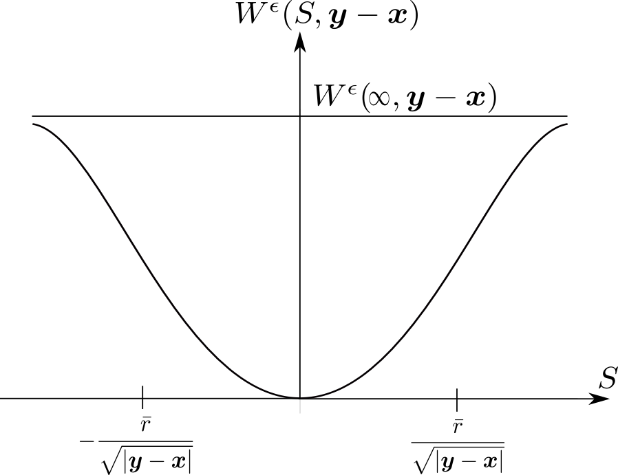
The potential Wϵ​(S,𝒚−𝒙)W^{\epsilon}(S,\boldsymbol{y}-\boldsymbol{x}) is of double well type and convex near the origin where it has one well and concave and bounded at infinity where it has the second well. Jϵ​(|𝒚−𝒙|)J^{\epsilon}(\left\lvert\boldsymbol{y}-\boldsymbol{x}\right\rvert) models the influence of separation between points 𝒚\boldsymbol{y} and 𝒙\boldsymbol{x}. We define JϵJ^{\epsilon} by rescaling J⁡(|𝝃|)J(\left\lvert\boldsymbol{\xi}\right\rvert), i.e. Jϵ​(|𝝃|)=J⁡(|𝝃|/ϵ)J^{\epsilon}(\left\lvert\boldsymbol{\xi}\right\rvert)=J(\left\lvert\boldsymbol{\xi}\right\rvert/\epsilon). Here JJ is zero outside the ball H1​(𝟎)H_{1}(\mathbf{0}) and satisfies 0≤J⁡(|𝝃|)≤M0\leq J(\left\lvert\boldsymbol{\xi}\right\rvert)\leq M for all 𝝃∈H1​(𝟎)\boldsymbol{\xi}\in H_{1}(\mathbf{0}). The domain function ω\omega enforces boundary conditions on ∂SWϵ\partial_{S}W^{\epsilon} at the boundary of the body DD. Here the boundary is denoted by ∂D\partial D and ω\omega is a nonnegative differentiable function 0≤ω≤10\leq\omega\leq 1. On the boundary ω=0\omega=0 and ω=1\omega=1 for points 𝒙\boldsymbol{x} inside DD with distance greater than ϵ\epsilon away from the boundary. We continue ω\omega by zero for all points outside DD.

The potential described in Equation 6 gives the convex-concave dependence of W⁡(S,𝒚−𝒙)W(S,\boldsymbol{y}-\boldsymbol{x}) on the strain SS for fixed 𝒚−𝒙\boldsymbol{y}-\boldsymbol{x}, see Figure 1. Initially the force is elastic for small strains and then softens as the strain becomes larger. The critical strain where the force between 𝒙\boldsymbol{x} and 𝒚\boldsymbol{y} begins to soften is given by Sc​(𝒚,𝒙):=r¯/|𝒚−𝒙|S_{c}(\boldsymbol{y},\boldsymbol{x}):=\bar{r}/\sqrt{\left\lvert\boldsymbol{y}-\boldsymbol{x}\right\rvert} and the force decreases monotonically for

|S⁡(𝒚,𝒙,𝒖)|>Sc.\displaystyle\left\lvert S(\boldsymbol{y},\boldsymbol{x};\boldsymbol{u})\right\rvert>S_{c}.

Here r¯\bar{r} is the inflection point of r:→f⁡(r2)r:\to f(r^{2}) and is the root of following equation

f′​(r2)+2​r2​f′′​(r2)=0.\displaystyle f^{\prime}({r}^{2})+2{r}^{2}f^{\prime\prime}({r}^{2})=0.
Refer to caption
Figure 1: Two point potential Wϵ​(S,𝒚−𝒙)W^{\epsilon}(S,\boldsymbol{y}-\boldsymbol{x}) as a function of strain SS for fixed 𝒚−𝒙\boldsymbol{y}-\boldsymbol{x}.
Refer to caption
Figure 2: Nonlocal force ∂SWϵ​(S,𝒚−𝒙)\partial_{S}W^{\epsilon}(S,\boldsymbol{y}-\boldsymbol{x}) as a function of strain SS for fixed 𝒚−𝒙\boldsymbol{y}-\boldsymbol{x}. Second derivative of Wϵ​(S,𝒚−𝒙)W^{\epsilon}(S,\boldsymbol{y}-\boldsymbol{x}) is zero at ±r¯/|𝒚−𝒙|\pm\bar{r}/\sqrt{|\boldsymbol{y}-\boldsymbol{x}|}.

2.2 Existence of solution

Let C0,γ​(D,ℝd)C^{0,\gamma}(D;\mathbb{R}^{d}) be the Hölder space with exponent γ∈(0,1]\gamma\in(0,1]. The closure of continuous functions with compact support on DD in the supremum norm is denoted by C0​(D)C_{0}(D). We identify functions in C0​(D)C_{0}(D) with their unique continuous extensions to D¯\overline{D}. It is easily seen that functions belonging to this space take the value zero on the boundary of DD, see e.g. [10]. We introduce C00,γ​(D)=C0,γ​(D)∩C0​(D)C_{0}^{0,\gamma}(D)=C^{0,\gamma}(D)\cap C_{0}(D). In this paper we extend all functions in C00,γ​(D)C_{0}^{0,\gamma}(D) by zero outside DD. The norm of 𝒖∈C00,γ​(D,ℝd)\boldsymbol{u}\in C^{0,\gamma}_{0}(D;\mathbb{R}^{d}) is taken to be

‖𝒖‖C0,γ​(D,ℝd)\displaystyle{\left\lVert\boldsymbol{u}\right\rVert}_{C^{0,\gamma}(D;\mathbb{R}^{d})} :=sup𝒙∈D|𝒖⁡(𝒙)|+[𝒖]C0,γ​(D,ℝd),\displaystyle:=\sup_{\boldsymbol{x}\in D}\left\lvert\boldsymbol{u}(\boldsymbol{x})\right\rvert+\left[\boldsymbol{u}\right]_{C^{0,\gamma}(D;\mathbb{R}^{d})},

where [𝒖]C0,γ​(D,ℝd)\left[\boldsymbol{u}\right]_{C^{0,\gamma}(D;\mathbb{R}^{d})} is the Hölder semi norm and given by

[𝒖]C0,γ​(D,ℝd)\displaystyle\left[\boldsymbol{u}\right]_{C^{0,\gamma}(D;\mathbb{R}^{d})} :=sup𝒙≠𝒚,𝒙,𝒚∈D|𝒖⁡(𝒙)−𝒖⁡(𝒚)||𝒙−𝒚|γ,\displaystyle:=\sup_{\begin{subarray}{c}\boldsymbol{x}\neq\boldsymbol{y},\\ \boldsymbol{x},\boldsymbol{y}\in D\end{subarray}}\dfrac{\left\lvert\boldsymbol{u}(\boldsymbol{x})-\boldsymbol{u}(\boldsymbol{y})\right\rvert}{\left\lvert\boldsymbol{x}-\boldsymbol{y}\right\rvert^{\gamma}},

and C00,γ​(D,ℝd)C^{0,\gamma}_{0}(D;\mathbb{R}^{d}) is a Banach space with this norm. Here we make the hypothesis that the domain function ω\omega belongs to C00,γ​(D,ℝd)C^{0,\gamma}_{0}(D;\mathbb{R}^{d}).

We write the evolution Equation 1 as an equivalent first order system with y1​(t)=𝒖​(t)y_{1}(t)=\boldsymbol{u}(t) and y2​(t)=𝒗​(t)y_{2}(t)=\boldsymbol{v}(t) with 𝒗⁡(t)=∂t𝒖⁡(t)\boldsymbol{v}(t)=\partial_{t}\boldsymbol{u}(t). Let y=(y1,y2)Ty=(y_{1},y_{2})^{T} where y1,y2∈C00,γ​(D,ℝd)y_{1},y_{2}\in C^{0,\gamma}_{0}(D;\mathbb{R}^{d}) and let Fϵ​(y,t)=(F1ϵ​(y,t),F2ϵ​(y,t))TF^{\epsilon}(y,t)=(F^{\epsilon}_{1}(y,t),F^{\epsilon}_{2}(y,t))^{T} such that

F1ϵ​(y,t)\displaystyle F^{\epsilon}_{1}(y,t) :=y2\displaystyle:=y_{2} (8)
F2ϵ​(y,t)\displaystyle F^{\epsilon}_{2}(y,t) :=−∇PDϵ(y1)+𝒃(t).\displaystyle:=-\boldsymbol{\nabla}PD^{\epsilon}(y_{1})+\boldsymbol{b}(t). (9)

The initial boundary value associated with the evolution Equation 1 is equivalent to the initial boundary value problem for the first order system given by

dd​t​y=Fϵ​(y,t),\displaystyle\dfrac{d}{dt}y=F^{\epsilon}(y,t), (10)

with initial condition given by y⁡(0)=(𝒖0,𝒗0)T∈C00,γ​(D,ℝd)×C00,γ​(D,ℝd)y(0)=(\boldsymbol{u}_{0},\boldsymbol{v}_{0})^{T}\in C^{0,\gamma}_{0}(D;\mathbb{R}^{d})\times C^{0,\gamma}_{0}(D;\mathbb{R}^{d}).

The function Fϵ​(y,t)F^{\epsilon}(y,t) satisfies the Lipschitz continuity given by the following theorem.

Proposition 1.

Lipschitz continuity and bound
Let X=C00,γ​(D,ℝd)×C00,γ​(D,ℝd)X=C^{0,\gamma}_{0}(D;\mathbb{R}^{d})\times C^{0,\gamma}_{0}(D;\mathbb{R}^{d}). The function Fϵ​(y,t)=(F1ϵ,F2ϵ)TF^{\epsilon}(y,t)=(F^{\epsilon}_{1},F^{\epsilon}_{2})^{T}, as defined in Equation 8 and Equation 9, is Lipschitz continuous in any bounded subset of XX. We have, for any y,z∈Xy,z\in X and t>0t>0,

‖Fϵ​(y,t)−Fϵ​(z,t)‖X\displaystyle{\left\lVert F^{\epsilon}(y,t)-F^{\epsilon}(z,t)\right\rVert}_{X}
≤(L1+L2​(‖ω‖C0,γ​(D)+‖y‖X+‖z‖X))ϵ2+α⁡(γ)​‖y−z‖X\displaystyle\leq\dfrac{\left(L_{1}+L_{2}\left(\|\omega\|_{C^{0,\gamma}(D)}+{\left\lVert y\right\rVert}_{X}+{\left\lVert z\right\rVert}_{X}\right)\right)}{\epsilon^{2+\alpha(\gamma)}}{\left\lVert y-z\right\rVert}_{X} (11)

where L1,L2L_{1},L_{2} are independent of 𝐮,𝐯\boldsymbol{u},\boldsymbol{v} and depend on peridynamic potential function ff and influence function JJ and the exponent α⁡(γ)\alpha(\gamma) is given by

α⁡(γ)={0if ​γ≥1/21/2−γif ​γ<1/2.\displaystyle\alpha(\gamma)=\begin{cases}0&\qquad\text{if }\gamma\geq 1/2\\ 1/2-\gamma&\qquad\text{if }\gamma<1/2.\end{cases}

Furthermore for any y∈Xy\in X and any t∈[0,T]t\in[0,T], we have the bound

‖Fϵ​(y,t)‖X\displaystyle{\left\lVert F^{\epsilon}(y,t)\right\rVert}_{X} ≤L3ϵ2+α⁡(γ)​(1+‖ω‖C0,γ​(D)+‖y‖X)+b\displaystyle\leq\dfrac{L_{3}}{\epsilon^{2+\alpha(\gamma)}}(1+\|\omega\|_{C^{0,\gamma}(D)}+{\left\lVert y\right\rVert}_{X})+b (12)

where b=supt‖𝐛⁡(t)‖C0,γ​(D,ℝd)b=\sup_{t}{\left\lVert\boldsymbol{b}(t)\right\rVert}_{C^{0,\gamma}(D;\mathbb{R}^{d})} and L3L_{3} is independent of yy.

We easily see that on choosing z=0z=0 in Proposition 1 that −∇PDϵ(𝒖)(𝒙)-\nabla PD^{\epsilon}(\boldsymbol{u})(\boldsymbol{x}) is in C0,γ​(D,ℝ3)C^{0,\gamma}(D;\mathbb{R}^{3}) provided that 𝒖\boldsymbol{u} belongs to C0,γ​(D,ℝ3)C^{0,\gamma}(D;\mathbb{R}^{3}). Since −∇PDϵ(𝒖)(𝒙)-\nabla PD^{\epsilon}(\boldsymbol{u})(\boldsymbol{x}) takes the value 00 on ∂D\partial D we conclude that −∇PDϵ(𝒖)(𝒙)-\nabla PD^{\epsilon}(\boldsymbol{u})(\boldsymbol{x}) belongs to C00,γ​(D,ℝ3)C^{0,\gamma}_{0}(D;\mathbb{R}^{3}).

In Theorem 6.1 of [23], the Lipschitz property of a peridynamic force is shown in X=L2​(D,ℝd)×L2​(D,ℝd)X=L^{2}(D;\mathbb{R}^{d})\times L^{2}(D;\mathbb{R}^{d}). It is given by

‖Fϵ​(y,t)−Fϵ​(z,t)‖X\displaystyle{\left\lVert F^{\epsilon}(y,t)-F^{\epsilon}(z,t)\right\rVert}_{X} ≤Lϵ2‖y−z‖X∀y,z∈X,∀t∈[0,T]\displaystyle\leq\dfrac{L}{\epsilon^{2}}{\left\lVert y-z\right\rVert}_{X}\qquad\forall y,z\in X,\forall t\in[0,T] (13)

for all y,z∈L02​(D,ℝd)2y,z\in L^{2}_{0}(D;\mathbb{R}^{d})^{2}. For this case LL does not depend on 𝒖,𝒗\boldsymbol{u},\boldsymbol{v}. We now state the existence theorem.

The following theorem gives the existence and uniqueness of solution in any given time domain I0=(−T,T)I_{0}=(-T,T).

Theorem 2.

Existence and uniqueness of Hölder solutions of cohesive dynamics over finite time intervals
For any initial condition x0∈X=C00,γ​(D,ℝd)×C00,γ​(D,ℝd)x_{0}\in X={C^{0,\gamma}_{0}(D;\mathbb{R}^{d})\times C^{0,\gamma}_{0}(D;\mathbb{R}^{d})}, time interval I0=(−T,T)I_{0}=(-T,T), and right hand side 𝐛⁡(t)\boldsymbol{b}(t) continuous in time for t∈I0t\in I_{0} such that 𝐛⁡(t)\boldsymbol{b}(t) satisfies supt∈I0‖𝐛⁡(t)‖C0,γ<∞\sup_{t\in I_{0}}{||\boldsymbol{b}(t)||_{C^{0,\gamma}}}<\infty, there is a unique solution y⁡(t)∈C1​(I0,X)y(t)\in C^{1}(I_{0};X) of

y⁡(t)=x0+∫0tFϵ​(y⁡(τ),τ)​𝑑τ,y(t)=x_{0}+\int_{0}^{t}F^{\epsilon}(y(\tau),\tau)\,d\tau,

or equivalently

y′​(t)=Fϵ​(y⁡(t),t),with y⁡(0)=x0,y^{\prime}(t)=F^{\epsilon}(y(t),t),\hbox{with $y(0)=x_{0}$},

where y⁡(t)y(t) and y′​(t)y^{\prime}(t) are Lipschitz continuous in time for t∈I0t\in I_{0}.

The proof of this theorem is given in section 4. We now describe the finite difference scheme and analyze its convergence to Hölder continuous solutions of cohesive dynamics.

3 Finite difference approximation

In this section, we present the finite difference scheme and compute the rate of convergence. We first consider the semi-discrete approximation and prove the bound on energy of semi-discrete evolution in terms of initial energy and the work done by body forces.

Let hh be the size of a mesh and Δ​t\Delta t be the size of time step. We will keep ϵ\epsilon fixed and assume that h<ϵ<1h<\epsilon<1. Let Dh=D∩(h​ℤ)dD_{h}=D\cap(h\mathbb{Z})^{d} be the discretization of material domain. Let i∈ℤdi\in\mathbb{Z}^{d} be the index such that 𝒙i=h​i∈D\boldsymbol{x}_{i}=hi\in D. Let UiU_{i} is the unit cell of volume hdh^{d} corresponding to the grid point 𝒙i\boldsymbol{x}_{i}. The exact solution evaluated at grid points is denoted by (𝒖i​(t),𝒗i​(t))(\boldsymbol{u}_{i}(t),\boldsymbol{v}_{i}(t)).

3.1 Time discretization

Let [0,T]∩(Δ​t​ℤ)[0,T]\cap(\Delta t\mathbb{Z}) be the discretization of time domain where Δ​t\Delta t is the size of time step. Denote fully discrete solution at (tk=k​Δ​t,𝒙i=i​h)(t^{k}=k\Delta t,\boldsymbol{x}_{i}=ih) as (𝒖^ik,𝒗^ik)(\hat{\boldsymbol{u}}^{k}_{i},\hat{\boldsymbol{v}}^{k}_{i}). Similarly, the exact solution evaluated at grid points is denoted by (𝒖ik,𝒗ik)(\boldsymbol{u}^{k}_{i},\boldsymbol{v}^{k}_{i}). We enforce boundary condition 𝒖^ik=𝟎\hat{\boldsymbol{u}}^{k}_{i}=\mathbf{0} for all 𝒙i∉D\boldsymbol{x}_{i}\notin D and for all kk.

We begin with the forward Euler time discretization, with respect to velocity, and the finite difference scheme for (𝒖^ik,𝒗^ik)(\hat{\boldsymbol{u}}^{k}_{i},\hat{\boldsymbol{v}}^{k}_{i}) is written

𝒖^ik+1−𝒖^ikΔ​t\displaystyle\dfrac{\hat{\boldsymbol{u}}^{k+1}_{i}-\hat{\boldsymbol{u}}^{k}_{i}}{\Delta t} =𝒗^ik+1\displaystyle=\hat{\boldsymbol{v}}^{k+1}_{i} (14)
𝒗^ik+1−𝒗^ikΔ​t\displaystyle\dfrac{\hat{\boldsymbol{v}}^{k+1}_{i}-\hat{\boldsymbol{v}}^{k}_{i}}{\Delta t} =−∇PDϵ(𝒖^k)(𝒙i)+𝒃ik\displaystyle=-\boldsymbol{\nabla}PD^{\epsilon}(\hat{\boldsymbol{u}}^{k})(\boldsymbol{x}_{i})+\boldsymbol{b}^{k}_{i} (15)

The scheme is complemented with the discretized initial conditions 𝒖^i0=(𝒖^0)i\hat{\boldsymbol{u}}^{0}_{i}=(\hat{\boldsymbol{u}}_{0})_{i} and 𝒗^i0=(𝒗^0)i\hat{\boldsymbol{v}}^{0}_{i}=(\hat{\boldsymbol{v}}_{0})_{i}. If we substitute Equation 14 into Equation 15, we get standard Central difference scheme in time for second order in time differential equation. Here we have assumed, without loss of generality, ρ=1\rho=1.

The piecewise constant extensions of the discrete sets {𝒖^ik}i∈ℤd\{\hat{\boldsymbol{u}}^{k}_{i}\}_{i\in\mathbb{Z}^{d}} and {𝒗^ik}i∈ℤd\{\hat{\boldsymbol{v}}^{k}_{i}\}_{i\in\mathbb{Z}^{d}} are given by

𝒖^k​(𝒙)\displaystyle\hat{\boldsymbol{u}}^{k}(\boldsymbol{x}) :=∑i,𝒙i∈D𝒖^ik​χUi​(𝒙)\displaystyle:=\sum_{i,\boldsymbol{x}_{i}\in D}\hat{\boldsymbol{u}}^{k}_{i}\chi_{U_{i}}(\boldsymbol{x})
𝒗^k​(𝒙)\displaystyle\hat{\boldsymbol{v}}^{k}(\boldsymbol{x}) :=∑i,𝒙i∈D𝒗^ik​χUi​(𝒙)\displaystyle:=\sum_{i,\boldsymbol{x}_{i}\in D}\hat{\boldsymbol{v}}^{k}_{i}\chi_{U_{i}}(\boldsymbol{x})

In this way we represent the finite difference solution as a piecewise constant function. We will show this function provides an L2L^{2} approximation of the exact solution.

Refer to caption
Figure 3: (a) Typical mesh of size hh. (b) Unit cell UiU_{i} corresponding to material point 𝒙i\boldsymbol{x}_{i}.

3.1.1 Convergence results

In this section we provide upper bounds on the rate of convergence of the discrete approximation to the solution of the peridynamic evolution. The L2L^{2} approximation error EkE^{k} at time tkt^{k}, for 0<tk≤T0<t^{k}\leq T is defined as

Ek\displaystyle E^{k} :=‖𝒖^k−𝒖k‖L2​(D,ℝd)+‖𝒗^k−𝒗k‖L2​(D,ℝd)\displaystyle:=\left\lVert\hat{\boldsymbol{u}}^{k}-\boldsymbol{u}^{k}\right\rVert_{L^{2}(D;\mathbb{R}^{d})}+\left\lVert\hat{\boldsymbol{v}}^{k}-\boldsymbol{v}^{k}\right\rVert_{L^{2}(D;\mathbb{R}^{d})}

The upper bound on the convergence rate of the approximation error is given by the following theorem.

Theorem 3.

Convergence of finite difference approximation (forward Euler time discretization)
Let ϵ>0\epsilon>0 be fixed. Let (𝐮,𝐯)(\boldsymbol{u},\boldsymbol{v}) be the solution of peridynamic equation Equation 10. We assume 𝐮,𝐯∈C2​([0,T],C00,γ​(D,ℝd))\boldsymbol{u},\boldsymbol{v}\in C^{2}([0,T];C^{0,\gamma}_{0}(D;\mathbb{R}^{d})). Then the finite difference scheme given by Equation 14 and Equation 15 is consistent in both time and spatial discretization and converges to the exact solution uniformly in time with respect to the L2​(D,ℝd)L^{2}(D;\mathbb{R}^{d}) norm. If we assume the error at the initial step is zero then the error EkE^{k} at time tkt^{k} is bounded and to leading order in the time step Δ​t\Delta t satisfies

sup0≤k≤T/Δ​tEk≤O⁡(Ct​Δ​t+Cs​hγϵ2),\displaystyle\sup_{0\leq k\leq T/\Delta t}E^{k}\leq O\left(C_{t}\Delta t+C_{s}\dfrac{h^{\gamma}}{\epsilon^{2}}\right), (16)

where constant CsC_{s} and CtC_{t} are independent of hh and Δ​t\Delta t and CsC_{s} depends on the Hölder norm of the solution and CtC_{t} depends on the L2L^{2} norms of time derivatives of the solution.

Here we have assumed the initial error to be zero for ease of exposition only.

We remark that the explicit constants leading to Equation 16 can be large. The inequality that delivers Equation 16 is given to leading order by

sup0≤k≤T/Δ​tEk≤exp⁡[T⁡(1+6​C¯/ϵ2)]​T​[Ct​Δ​t+(Cs/ϵ2)​hγ],\displaystyle\sup_{0\leq k\leq T/\Delta t}E^{k}\leq\exp\left[T(1+6\bar{C}/\epsilon^{2})\right]T\left[C_{t}\Delta t+(C_{s}/\epsilon^{2})h^{\gamma}\right], (17)

where the constants C¯\bar{C}, CtC_{t} and CsC_{s} are given by Equation 35, Equation 37, and Equation 38. The explicit constant CtC_{t} depends on the spatial L2L^{2} norm of the time derivatives of the solution and CsC_{s} depends on the spatial Hölder continuity of the solution and the constant C¯\bar{C}. This constant is bounded independently of horizon ϵ\epsilon. Although the constants are necessarily pessimistic they deliver a-priori error estimates and an example is discussed in section 6.

An identical convergence rate can be established for the general one step scheme and we state it below.

Theorem 4.

Convergence of finite difference approximation (General single step time discretization)
Let us assume that the hypothesis of Theorem 3 holds. Fix θ∈[0,1]\theta\in[0,1], and let (𝐮^k,𝐯^k)T(\hat{\boldsymbol{u}}^{k},\hat{\boldsymbol{v}}^{k})^{T} be the solution of following finite difference equation

𝒖^ik+1−𝒖^ikΔ​t\displaystyle\dfrac{\hat{\boldsymbol{u}}^{k+1}_{i}-\hat{\boldsymbol{u}}^{k}_{i}}{\Delta t} =(1−θ)​𝒗^ik+θ​𝒗^ik+1\displaystyle=(1-\theta)\hat{\boldsymbol{v}}^{k}_{i}+\theta\hat{\boldsymbol{v}}^{k+1}_{i} (18)
𝒗^ik+1−𝒗^ikΔ​t\displaystyle\dfrac{\hat{\boldsymbol{v}}^{k+1}_{i}-\hat{\boldsymbol{v}}^{k}_{i}}{\Delta t} =(1−θ)(−∇PDϵ(𝒖^k)(𝒙i)+𝒃ik)+θ(−∇PDϵ(𝒖^k+1)(𝒙i)+𝒃ik+1).\displaystyle=(1-\theta)\left(-\boldsymbol{\nabla}PD^{\epsilon}(\hat{\boldsymbol{u}}^{k})(\boldsymbol{x}_{i})+\boldsymbol{b}^{k}_{i}\right)+\theta\left(-\boldsymbol{\nabla}PD^{\epsilon}(\hat{\boldsymbol{u}}^{k+1})(\boldsymbol{x}_{i})+\boldsymbol{b}^{k+1}_{i}\right). (19)

Then, for any fixed θ∈[0,1]\theta\in[0,1], there exists a constant K>0K>0 independent of (𝐮^k,𝐯^k)T(\hat{\boldsymbol{u}}^{k},\hat{\boldsymbol{v}}^{k})^{T} and (𝐮k,𝐯k)T(\boldsymbol{u}^{k},\boldsymbol{v}^{k})^{T}, such that for Δ​t<K​ϵ2\Delta t<K{\epsilon^{2}} the finite difference scheme given by Equation 18 and Equation 19 is consistent in time and spatial discretization. if we assume the error at the initial step is zero then the error EkE^{k} at time tkt^{k} is bounded and satisfies

sup0≤k≤T/Δ​tEk≤O⁡(Ct​Δ​t+Cs​hγϵ2).\displaystyle\sup_{0\leq k\leq T/\Delta t}E^{k}\leq O\left(C_{t}\Delta t+C_{s}\dfrac{h^{\gamma}}{\epsilon^{2}}\right).

The constant KK is given by the explicit formula K=1/C¯K=1/\bar{C} where C¯\bar{C} is described by equation Equation 35. Furthermore for the Crank Nicholson scheme, θ=1/2\theta=1/2, if we assume the solutions 𝐮,𝐯\boldsymbol{u},\boldsymbol{v} belong to C3​([0,T],C00,γ​(D,ℝd))C^{3}([0,T];C^{0,\gamma}_{0}(D;\mathbb{R}^{d})), then the approximation error EkE^{k} satisfies

sup0≤k≤T/Δ​tEk≤O⁡(C¯t​(Δ​t)2+Cs​hγϵ2),\displaystyle\sup_{0\leq k\leq T/\Delta t}E^{k}\leq O\left(\bar{C}_{t}(\Delta t)^{2}+C_{s}\dfrac{h^{\gamma}}{\epsilon^{2}}\right),

where C¯t\bar{C}_{t} is independent of Δ​t\Delta t and hh and is given by Equation 49.

As before we assume that the error in the initial data is zero for ease of exposition. The proofs of Theorem 3 and Theorem 4 are given in the following sections.

Remark. In Theorem 4, we have stated a condition on Δ​t\Delta t for which the convergence estimate holds. This condition naturally occurs in the analysis and is related to the Lipschitz continuity of the peridnamic force with respect to the L2L^{2} norm, see Equation 41.

3.1.2 Error analysis

Theorem 3and Theorem 4 are proved along similar lines. In both cases we define the L2L^{2}-projections of the actual solutions onto the space of piecewise constant functions defined over the cells UiU_{i}. These are given as follows. Let (𝒖~ik,𝒗~ik)(\tilde{\boldsymbol{u}}^{k}_{i},\tilde{\boldsymbol{v}}^{k}_{i}) be the average of the exact solution (𝒖k,𝒗k)(\boldsymbol{u}^{k},\boldsymbol{v}^{k}) in the unit cell UiU_{i} given by

𝒖~ik\displaystyle\tilde{\boldsymbol{u}}^{k}_{i} :=1hd​∫Ui𝒖k​(𝒙)​𝑑𝒙\displaystyle:=\dfrac{1}{h^{d}}\int_{U_{i}}\boldsymbol{u}^{k}(\boldsymbol{x})d\boldsymbol{x}
𝒗~ik\displaystyle\tilde{\boldsymbol{v}}^{k}_{i} :=1hd​∫Ui𝒗k​(𝒙)​𝑑𝒙\displaystyle:=\dfrac{1}{h^{d}}\int_{U_{i}}\boldsymbol{v}^{k}(\boldsymbol{x})d\boldsymbol{x}

and the L2L^{2} projection of the solution onto piecewise constant functions are (𝒖~k,𝒗~k)(\tilde{\boldsymbol{u}}^{k},\tilde{\boldsymbol{v}}^{k}) given by

𝒖~k​(𝒙)\displaystyle\tilde{\boldsymbol{u}}^{k}(\boldsymbol{x}) :=∑i,𝒙i∈D𝒖~ik​χUi​(𝒙)\displaystyle:=\sum_{i,\boldsymbol{x}_{i}\in D}\tilde{\boldsymbol{u}}^{k}_{i}\chi_{U_{i}}(\boldsymbol{x}) (20)
𝒗~k​(𝒙)\displaystyle\tilde{\boldsymbol{v}}^{k}(\boldsymbol{x}) :=∑i,𝒙i∈D𝒗~ik​χUi​(𝒙)\displaystyle:=\sum_{i,\boldsymbol{x}_{i}\in D}\tilde{\boldsymbol{v}}^{k}_{i}\chi_{U_{i}}(\boldsymbol{x}) (21)

The error between (𝒖^k,𝒗^k)T(\hat{\boldsymbol{u}}^{k},\hat{\boldsymbol{v}}^{k})^{T} with (𝒖⁡(tk),𝒗⁡(tk))T(\boldsymbol{u}(t^{k}),\boldsymbol{v}(t^{k}))^{T} is now split into two parts. From the triangle inequality, we have

‖𝒖^k−𝒖⁡(tk)‖L2​(D,ℝd)\displaystyle\left\lVert\hat{\boldsymbol{u}}^{k}-\boldsymbol{u}(t^{k})\right\rVert_{L^{2}(D;\mathbb{R}^{d})} ≤‖𝒖^k−𝒖~k‖L2​(D,ℝd)+‖𝒖~k−𝒖k‖L2​(D,ℝd)\displaystyle\leq\left\lVert\hat{\boldsymbol{u}}^{k}-\tilde{\boldsymbol{u}}^{k}\right\rVert_{L^{2}(D;\mathbb{R}^{d})}+\left\lVert\tilde{\boldsymbol{u}}^{k}-\boldsymbol{u}^{k}\right\rVert_{L^{2}(D;\mathbb{R}^{d})}
‖𝒗^k−𝒗⁡(tk)‖L2​(D,ℝd)\displaystyle\left\lVert\hat{\boldsymbol{v}}^{k}-\boldsymbol{v}(t^{k})\right\rVert_{L^{2}(D;\mathbb{R}^{d})} ≤‖𝒗^k−𝒗~k‖L2​(D,ℝd)+‖𝒗~k−𝒗k‖L2​(D,ℝd)\displaystyle\leq\left\lVert\hat{\boldsymbol{v}}^{k}-\tilde{\boldsymbol{v}}^{k}\right\rVert_{L^{2}(D;\mathbb{R}^{d})}+\left\lVert\tilde{\boldsymbol{v}}^{k}-\boldsymbol{v}^{k}\right\rVert_{L^{2}(D;\mathbb{R}^{d})}

In subsubsection 3.1.3 and subsection 3.2 we will show that the error between the L2L^{2} projections of the actual solution and the discrete approximation for both forward Euler and implicit one step methods decay according to

sup0≤k≤T/Δ​t(‖𝒖^k−𝒖~k‖L2​(D,ℝd)+‖𝒗^k−𝒗~k‖L2​(D,ℝd))\displaystyle\sup_{0\leq k\leq T/\Delta t}\left(\left\lVert\hat{\boldsymbol{u}}^{k}-\tilde{\boldsymbol{u}}^{k}\right\rVert_{L^{2}(D;\mathbb{R}^{d})}+\left\lVert\hat{\boldsymbol{v}}^{k}-\tilde{\boldsymbol{v}}^{k}\right\rVert_{L^{2}(D;\mathbb{R}^{d})}\right) =O⁡(Δ​t+hγϵ2).\displaystyle=O\left(\Delta t+\dfrac{h^{\gamma}}{\epsilon^{2}}\right). (22)

In what follows we can estimate the terms

‖𝒖~k−𝒖⁡(tk)‖L2​ and ​‖𝒗~k−𝒗⁡(tk)‖L2\displaystyle\left\lVert\tilde{\boldsymbol{u}}^{k}-\boldsymbol{u}(t^{k})\right\rVert_{L^{2}}\hbox{ and }\left\lVert\tilde{\boldsymbol{v}}^{k}-\boldsymbol{v}(t^{k})\right\rVert_{L^{2}} (23)

and show they go to zero at a rate of hγh^{\gamma} uniformly in time. The estimates given by Equation 22 together with the O⁡(hγ)O(h^{\gamma}) estimates for Equation 23 establish Theorem 3 and Theorem 4. We now establish the L2L^{2} estimates for the differences 𝒖~k−𝒖⁡(tk)\tilde{\boldsymbol{u}}^{k}-\boldsymbol{u}(t^{k}) and 𝒗~k−𝒗⁡(tk)\tilde{\boldsymbol{v}}^{k}-\boldsymbol{v}(t^{k}).

We write

‖𝒖~k−𝒖k‖L2​(D,ℝd)2\displaystyle\left\lVert\tilde{\boldsymbol{u}}^{k}-\boldsymbol{u}^{k}\right\rVert_{L^{2}(D;\mathbb{R}^{d})}^{2}
=∑i,𝒙i∈D∫Ui|𝒖~k​(𝒙)−𝒖k​(𝒙)|2​𝑑𝒙\displaystyle=\sum_{i,\boldsymbol{x}_{i}\in D}\int_{U_{i}}\left\lvert\tilde{\boldsymbol{u}}^{k}(\boldsymbol{x})-\boldsymbol{u}^{k}(\boldsymbol{x})\right\rvert^{2}d\boldsymbol{x}
=∑i,𝒙i∈D∫Ui|1hd​∫Ui(𝒖k​(𝒚)−𝒖k​(𝒙))​𝑑𝒚|2​𝑑𝒙\displaystyle=\sum_{i,\boldsymbol{x}_{i}\in D}\int_{U_{i}}\left\lvert\dfrac{1}{h^{d}}\int_{U_{i}}(\boldsymbol{u}^{k}(\boldsymbol{y})-\boldsymbol{u}^{k}(\boldsymbol{x}))d\boldsymbol{y}\right\rvert^{2}d\boldsymbol{x}
=∑i,𝒙i∈D∫Ui[1h2​d​∫Ui∫Ui(𝒖k​(𝒚)−𝒖k​(𝒙))⋅(𝒖k​(𝒛)−𝒖k​(𝒙))​𝑑𝒚​𝑑𝒛]​𝑑𝒙\displaystyle=\sum_{i,\boldsymbol{x}_{i}\in D}\int_{U_{i}}\left[\dfrac{1}{h^{2d}}\int_{U_{i}}\int_{U_{i}}(\boldsymbol{u}^{k}(\boldsymbol{y})-\boldsymbol{u}^{k}(\boldsymbol{x}))\cdot(\boldsymbol{u}^{k}(\boldsymbol{z})-\boldsymbol{u}^{k}(\boldsymbol{x}))d\boldsymbol{y}d\boldsymbol{z}\right]d\boldsymbol{x}
≤∑i,𝒙i∈D∫Ui[1hd​∫Ui|𝒖k​(𝒚)−𝒖k​(𝒙)|2​𝑑𝒚]​𝑑𝒙\displaystyle\leq\sum_{i,\boldsymbol{x}_{i}\in D}\int_{U_{i}}\left[\dfrac{1}{h^{d}}\int_{U_{i}}\left\lvert\boldsymbol{u}^{k}(\boldsymbol{y})-\boldsymbol{u}^{k}(\boldsymbol{x})\right\rvert^{2}d\boldsymbol{y}\right]d\boldsymbol{x} (24)

where we used Cauchy’s inequality and Jensen’s inequality. For 𝒙,𝒚∈Ui\boldsymbol{x},\boldsymbol{y}\in U_{i}, |𝒙−𝒚|≤c​h\left\lvert\boldsymbol{x}-\boldsymbol{y}\right\rvert\leq ch, where c=2c=\sqrt{2} for d=2d=2 and c=3c=\sqrt{3} for d=3d=3. Since 𝒖∈C00,γ\boldsymbol{u}\in C^{0,\gamma}_{0} we have

|𝒖k​(𝒙)−𝒖k​(𝒚)|\displaystyle\left\lvert\boldsymbol{u}^{k}(\boldsymbol{x})-\boldsymbol{u}^{k}(\boldsymbol{y})\right\rvert =|𝒙−𝒚|γ​|𝒖k​(𝒚)−𝒖k​(𝒙)||𝒙−𝒚|γ\displaystyle=\left\lvert\boldsymbol{x}-\boldsymbol{y}\right\rvert^{\gamma}\dfrac{\left\lvert\boldsymbol{u}^{k}(\boldsymbol{y})-\boldsymbol{u}^{k}(\boldsymbol{x})\right\rvert}{\left\lvert\boldsymbol{x}-\boldsymbol{y}\right\rvert^{\gamma}}
≤cγ​hγ​‖𝒖k‖C0,γ​(D,ℝd)≤cγ​hγ​supt‖𝒖⁡(t)‖C0,γ​(D,ℝd)\displaystyle\leq c^{\gamma}h^{\gamma}{\left\lVert\boldsymbol{u}^{k}\right\rVert}_{C^{0,\gamma}(D;\mathbb{R}^{d})}\leq c^{\gamma}h^{\gamma}\sup_{t}{\left\lVert\boldsymbol{u}(t)\right\rVert}_{C^{0,\gamma}(D;\mathbb{R}^{d})} (25)

and substitution in Equation 24 gives

‖𝒖~k−𝒖k‖L2​(D,ℝd)2\displaystyle\left\lVert\tilde{\boldsymbol{u}}^{k}-\boldsymbol{u}^{k}\right\rVert_{L^{2}(D;\mathbb{R}^{d})}^{2} ≤c2​γ​h2​γ​∑i,𝒙i∈D∫Uid​𝒙​(supt‖𝒖⁡(t)‖C0,γ​(D,ℝd))2\displaystyle\leq c^{2\gamma}h^{2\gamma}\sum_{i,\boldsymbol{x}_{i}\in D}\int_{U_{i}}d\boldsymbol{x}\left(\sup_{t}{\left\lVert\boldsymbol{u}(t)\right\rVert}_{C^{0,\gamma}(D;\mathbb{R}^{d})}\right)^{2}
≤c2​γ​|D|​h2​γ​(supt‖𝒖⁡(t)‖C0,γ​(D,ℝd))2.\displaystyle\leq c^{2\gamma}|D|h^{2\gamma}\left(\sup_{t}{\left\lVert\boldsymbol{u}(t)\right\rVert}_{C^{0,\gamma}(D;\mathbb{R}^{d})}\right)^{2}.

A similar estimate can be derived for ‖𝒗~k−𝒗k‖L2||\tilde{\boldsymbol{v}}^{k}-\boldsymbol{v}^{k}||_{L^{2}} and substitution of the estimates into Equation 23 gives

supk(‖𝒖~k−𝒖⁡(tk)‖L2​(D,ℝd)+‖𝒗~k−𝒗⁡(tk)‖L2​(D,ℝd))=O⁡(hγ).\displaystyle\sup_{k}\left(\left\lVert\tilde{\boldsymbol{u}}^{k}-\boldsymbol{u}(t^{k})\right\rVert_{L^{2}(D;\mathbb{R}^{d})}+\left\lVert\tilde{\boldsymbol{v}}^{k}-\boldsymbol{v}(t^{k})\right\rVert_{L^{2}(D;\mathbb{R}^{d})}\right)=O(h^{\gamma}).

In the next section we establish the error estimate Equation 22 for both forward Euler and general one step schemes in subsubsection 3.1.3 and subsection 3.2.

3.1.3 Error analysis for approximation of L2L^{2} projection of the the exact solution

In this sub-section, we estimate the difference between approximate solution (𝒖^k,𝒗^k)(\hat{\boldsymbol{u}}^{k},\hat{\boldsymbol{v}}^{k}) and the L2L^{2} projection of the exact solution onto piece wise constant functions given by (𝒖~k,𝒗~k)(\tilde{\boldsymbol{u}}^{k},\tilde{\boldsymbol{v}}^{k}), see Equation 20 and Equation 21 . Let the differences be denoted by 𝒆k​(u):=𝒖^k−𝒖~k\boldsymbol{e}^{k}(u):=\hat{\boldsymbol{u}}^{k}-\tilde{\boldsymbol{u}}^{k} and 𝒆k​(v):=𝒗^k−𝒗~k\boldsymbol{e}^{k}(v):=\hat{\boldsymbol{v}}^{k}-\tilde{\boldsymbol{v}}^{k} and their evaluation at grid points are 𝒆ik​(u):=𝒖^ik−𝒖~ik\boldsymbol{e}^{k}_{i}(u):=\hat{\boldsymbol{u}}^{k}_{i}-\tilde{\boldsymbol{u}}^{k}_{i} and 𝒆ik​(v):=𝒗^ik−𝒗~ik\boldsymbol{e}^{k}_{i}(v):=\hat{\boldsymbol{v}}^{k}_{i}-\tilde{\boldsymbol{v}}^{k}_{i}. Subtracting (𝒖~ik+1−𝒖~ik)/Δ​t(\tilde{\boldsymbol{u}}^{k+1}_{i}-\tilde{\boldsymbol{u}}^{k}_{i})/\Delta t from Equation 14 gives

𝒖^ik+1−𝒖^ikΔ​t−𝒖~ik+1−𝒖~ikΔ​t\displaystyle\dfrac{\hat{\boldsymbol{u}}^{k+1}_{i}-\hat{\boldsymbol{u}}^{k}_{i}}{\Delta t}-\dfrac{\tilde{\boldsymbol{u}}^{k+1}_{i}-\tilde{\boldsymbol{u}}^{k}_{i}}{\Delta t}
=𝒗^ik+1−𝒖~ik+1−𝒖~ikΔ​t\displaystyle=\hat{\boldsymbol{v}}^{k+1}_{i}-\dfrac{\tilde{\boldsymbol{u}}^{k+1}_{i}-\tilde{\boldsymbol{u}}^{k}_{i}}{\Delta t}
=𝒗^ik+1−𝒗~ik+1+(𝒗~ik+1−∂𝒖~ik+1∂t)+(∂𝒖~ik+1∂t−𝒖~ik+1−𝒖~ikΔ​t).\displaystyle=\hat{\boldsymbol{v}}^{k+1}_{i}-\tilde{\boldsymbol{v}}^{k+1}_{i}+\left(\tilde{\boldsymbol{v}}^{k+1}_{i}-\dfrac{\partial\tilde{\boldsymbol{u}}^{k+1}_{i}}{\partial t}\right)+\left(\dfrac{\partial\tilde{\boldsymbol{u}}^{k+1}_{i}}{\partial t}-\dfrac{\tilde{\boldsymbol{u}}^{k+1}_{i}-\tilde{\boldsymbol{u}}^{k}_{i}}{\Delta t}\right).

Taking the average over unit cell UiU_{i} of the exact peridynamic equation Equation 10 at time tkt^{k}, we will get 𝒗~ik+1−∂𝒖~ik+1∂t=0\tilde{\boldsymbol{v}}^{k+1}_{i}-\dfrac{\partial\tilde{\boldsymbol{u}}^{k+1}_{i}}{\partial t}=0. Therefore, the equation for 𝒆ik​(u)\boldsymbol{e}^{k}_{i}(u) is given by

𝒆ik+1​(u)=𝒆ik​(u)+Δ​t​𝒆ik+1​(v)+Δ​t​τik​(u),\displaystyle\boldsymbol{e}^{k+1}_{i}(u)=\boldsymbol{e}^{k}_{i}(u)+\Delta t\boldsymbol{e}^{k+1}_{i}(v)+\Delta t\tau^{k}_{i}(u), (26)

where we identify the discretization error as

τik​(u)\displaystyle\tau^{k}_{i}(u) :=∂𝒖~ik+1∂t−𝒖~ik+1−𝒖~ikΔ​t.\displaystyle:=\dfrac{\partial\tilde{\boldsymbol{u}}^{k+1}_{i}}{\partial t}-\dfrac{\tilde{\boldsymbol{u}}^{k+1}_{i}-\tilde{\boldsymbol{u}}^{k}_{i}}{\Delta t}. (27)

Similarly, we subtract (𝒗~ik+1−𝒗~ik)/Δ​t(\tilde{\boldsymbol{v}}^{k+1}_{i}-\tilde{\boldsymbol{v}}^{k}_{i})/\Delta t from Equation 15 and add and subtract terms to get

𝒗^ik+1−𝒗^ikΔ​t−𝒗~ik+1−𝒗~ikΔ​t\displaystyle\dfrac{\hat{\boldsymbol{v}}^{k+1}_{i}-\hat{\boldsymbol{v}}^{k}_{i}}{\Delta t}-\dfrac{\tilde{\boldsymbol{v}}^{k+1}_{i}-\tilde{\boldsymbol{v}}^{k}_{i}}{\Delta t} =−∇PDϵ(𝒖^k)(𝒙i)+𝒃ik−∂𝒗ik∂t+(∂𝒗ik∂t−𝒗~ik+1−𝒗~ikΔ​t)\displaystyle=-\boldsymbol{\nabla}PD^{\epsilon}(\hat{\boldsymbol{u}}^{k})(\boldsymbol{x}_{i})+\boldsymbol{b}^{k}_{i}-\dfrac{\partial\boldsymbol{v}^{k}_{i}}{\partial t}+\left(\dfrac{\partial\boldsymbol{v}^{k}_{i}}{\partial t}-\dfrac{\tilde{\boldsymbol{v}}^{k+1}_{i}-\tilde{\boldsymbol{v}}^{k}_{i}}{\Delta t}\right)
=−∇PDϵ(𝒖^k)(𝒙i)+𝒃ik−∂𝒗ik∂t\displaystyle=-\boldsymbol{\nabla}PD^{\epsilon}(\hat{\boldsymbol{u}}^{k})(\boldsymbol{x}_{i})+\boldsymbol{b}^{k}_{i}-\dfrac{\partial\boldsymbol{v}^{k}_{i}}{\partial t}
+(∂𝒗~ik∂t−𝒗~ik+1−𝒗~ikΔ​t)+(∂𝒗ik∂t−∂𝒗~ik∂t),\displaystyle\quad+\left(\dfrac{\partial\tilde{\boldsymbol{v}}^{k}_{i}}{\partial t}-\dfrac{\tilde{\boldsymbol{v}}^{k+1}_{i}-\tilde{\boldsymbol{v}}^{k}_{i}}{\Delta t}\right)+\left(\dfrac{\partial\boldsymbol{v}^{k}_{i}}{\partial t}-\dfrac{\partial\tilde{\boldsymbol{v}}^{k}_{i}}{\partial t}\right), (28)

where we identify τik​(v)\tau^{k}_{i}(v) as follows

τik​(v)\displaystyle\tau^{k}_{i}(v) :=∂𝒗~ik∂t−𝒗~ik+1−𝒗~ikΔ​t.\displaystyle:=\dfrac{\partial\tilde{\boldsymbol{v}}^{k}_{i}}{\partial t}-\dfrac{\tilde{\boldsymbol{v}}^{k+1}_{i}-\tilde{\boldsymbol{v}}^{k}_{i}}{\Delta t}. (29)

Note that in τk​(u)\tau^{k}(u) we have ∂𝒖~ik+1∂t\dfrac{\partial\tilde{\boldsymbol{u}}^{k+1}_{i}}{\partial t} and from the exact peridynamic equation, we have

𝒃ik−∂𝒗ik∂t=∇PDϵ(𝒖k)(𝒙i).\displaystyle\boldsymbol{b}^{k}_{i}-\dfrac{\partial\boldsymbol{v}^{k}_{i}}{\partial t}=\boldsymbol{\nabla}PD^{\epsilon}(\boldsymbol{u}^{k})(\boldsymbol{x}_{i}). (30)

Combining subsubsection 3.1.3, Equation 29, and Equation 30, to get

𝒆ik+1​(v)\displaystyle\boldsymbol{e}^{k+1}_{i}(v) =𝒆ik​(v)+Δ​t​τik​(v)+Δ​t​(∂𝒗ik∂t−∂𝒗~ik∂t)\displaystyle=\boldsymbol{e}^{k}_{i}(v)+\Delta t\tau^{k}_{i}(v)+\Delta t\left(\dfrac{\partial\boldsymbol{v}^{k}_{i}}{\partial t}-\dfrac{\partial\tilde{\boldsymbol{v}}^{k}_{i}}{\partial t}\right)
+Δt(−∇PDϵ(𝒖^k)(𝒙i)+∇PDϵ(𝒖k)(𝒙i))\displaystyle\quad+\Delta t\left(-\boldsymbol{\nabla}PD^{\epsilon}(\hat{\boldsymbol{u}}^{k})(\boldsymbol{x}_{i})+\boldsymbol{\nabla}PD^{\epsilon}(\boldsymbol{u}^{k})(\boldsymbol{x}_{i})\right)
=𝒆ik​(v)+Δ​t​τik​(v)+Δ​t​(∂𝒗ik∂t−∂𝒗~ik∂t)\displaystyle=\boldsymbol{e}^{k}_{i}(v)+\Delta t\tau^{k}_{i}(v)+\Delta t\left(\dfrac{\partial\boldsymbol{v}^{k}_{i}}{\partial t}-\dfrac{\partial\tilde{\boldsymbol{v}}^{k}_{i}}{\partial t}\right)
+Δt(−∇PDϵ(𝒖^k)(𝒙i)+∇PDϵ(𝒖~k)(𝒙i))\displaystyle\quad+\Delta t\left(-\boldsymbol{\nabla}PD^{\epsilon}(\hat{\boldsymbol{u}}^{k})(\boldsymbol{x}_{i})+\boldsymbol{\nabla}PD^{\epsilon}(\tilde{\boldsymbol{u}}^{k})(\boldsymbol{x}_{i})\right)
+Δt(−∇PDϵ(𝒖~k)(𝒙i)+∇PDϵ(𝒖k)(𝒙i)).\displaystyle\quad+\Delta t\left(-\boldsymbol{\nabla}PD^{\epsilon}(\tilde{\boldsymbol{u}}^{k})(\boldsymbol{x}_{i})+\boldsymbol{\nabla}PD^{\epsilon}(\boldsymbol{u}^{k})(\boldsymbol{x}_{i})\right).

The spatial discretization error σik​(u)\sigma^{k}_{i}(u) and σik​(v)\sigma^{k}_{i}(v) is given by

σik​(u)\displaystyle\sigma^{k}_{i}(u) :=(−∇PDϵ(𝒖~k)(𝒙i)+∇PDϵ(𝒖k)(𝒙i))\displaystyle:=\left(-\boldsymbol{\nabla}PD^{\epsilon}(\tilde{\boldsymbol{u}}^{k})(\boldsymbol{x}_{i})+\boldsymbol{\nabla}PD^{\epsilon}(\boldsymbol{u}^{k})(\boldsymbol{x}_{i})\right) (31)
σik​(v)\displaystyle\sigma^{k}_{i}(v) :=∂𝒗ik∂t−∂𝒗~ik∂t.\displaystyle:=\dfrac{\partial\boldsymbol{v}^{k}_{i}}{\partial t}-\dfrac{\partial\tilde{\boldsymbol{v}}^{k}_{i}}{\partial t}. (32)

We finally have

𝒆ik+1​(v)\displaystyle\boldsymbol{e}^{k+1}_{i}(v) =𝒆ik​(v)+Δ​t​(τik​(v)+σik​(u)+σik​(v))\displaystyle=\boldsymbol{e}^{k}_{i}(v)+\Delta t\left(\tau^{k}_{i}(v)+\sigma^{k}_{i}(u)+\sigma^{k}_{i}(v)\right)
+Δt(−∇PDϵ(𝒖^k)(𝒙i)+∇PDϵ(𝒖~k)(𝒙i)).\displaystyle\quad+\Delta t\left(-\boldsymbol{\nabla}PD^{\epsilon}(\hat{\boldsymbol{u}}^{k})(\boldsymbol{x}_{i})+\boldsymbol{\nabla}PD^{\epsilon}(\tilde{\boldsymbol{u}}^{k})(\boldsymbol{x}_{i})\right). (33)

We now show the consistency and stability properties of the numerical scheme.

3.1.4 Consistency

We deal with the error in time discretization and the error in spatial discretization error separately. The time discretization error follows easily using the Taylor’s series while spatial the discretization error uses properties of the nonlinear peridynamic force.

Time discretization: We first estimate the time discretization error. A Taylor series expansion is used to estimate τik​(u)\tau^{k}_{i}(u) as follows

τik​(u)\displaystyle\tau^{k}_{i}(u) =1hd​∫Ui(∂𝒖k​(𝒙)∂t−𝒖k+1​(𝒙)−𝒖k​(𝒙)Δ​t)​𝑑𝒙\displaystyle=\dfrac{1}{h^{d}}\int_{U_{i}}\left(\dfrac{\partial\boldsymbol{u}^{k}(\boldsymbol{x})}{\partial t}-\dfrac{\boldsymbol{u}^{k+1}(\boldsymbol{x})-\boldsymbol{u}^{k}(\boldsymbol{x})}{\Delta t}\right)d\boldsymbol{x}
=1hd​∫Ui(−12​∂2𝒖k​(𝒙)∂t2​Δ​t+O⁡((Δ​t)2))​𝑑𝒙.\displaystyle=\dfrac{1}{h^{d}}\int_{U_{i}}\left(-\dfrac{1}{2}\dfrac{\partial^{2}\boldsymbol{u}^{k}(\boldsymbol{x})}{\partial t^{2}}\Delta t+O((\Delta t)^{2})\right)d\boldsymbol{x}.

Computing the L2L^{2} norm of τik​(u)\tau^{k}_{i}(u) and using Jensen’s inequality gives

‖τk​(u)‖L2​(D,ℝd)\displaystyle\left\lVert\tau^{k}(u)\right\rVert_{L^{2}(D;\mathbb{R}^{d})} ≤Δ​t2​‖∂2𝒖k∂t2‖L2​(D,ℝd)+O⁡((Δ​t)2)\displaystyle\leq\frac{\Delta t}{2}\left\lVert\dfrac{\partial^{2}\boldsymbol{u}^{k}}{\partial t^{2}}\right\rVert_{L^{2}(D;\mathbb{R}^{d})}+O((\Delta t)^{2})
≤Δ​t2​supt‖∂2𝒖⁡(t)∂t2‖L2​(D,ℝd)+O⁡((Δ​t)2).\displaystyle\leq\frac{\Delta t}{2}\sup_{t}\left\lVert\dfrac{\partial^{2}\boldsymbol{u}(t)}{\partial t^{2}}\right\rVert_{L^{2}(D;\mathbb{R}^{d})}+O((\Delta t)^{2}).

Similarly, we have

‖τk​(v)‖L2​(D,ℝd)=Δ​t2​supt‖∂2𝒗⁡(t)∂t2‖L2​(D,ℝd)+O⁡((Δ​t)2).\displaystyle\left\lVert\tau^{k}(v)\right\rVert_{L^{2}(D;\mathbb{R}^{d})}=\frac{\Delta t}{2}\sup_{t}\left\lVert\dfrac{\partial^{2}\boldsymbol{v}(t)}{\partial t^{2}}\right\rVert_{L^{2}(D;\mathbb{R}^{d})}+O((\Delta t)^{2}).

Spatial discretization: We now estimate the spatial discretization error. Substituting the definition of 𝒗~k\tilde{\boldsymbol{v}}^{k} and following the similar steps employed in subsubsection 3.1.2, gives

|σik​(v)|\displaystyle\left\lvert\sigma^{k}_{i}(v)\right\rvert =|∂𝒗ik∂t−1hd​∫Ui∂𝒗k​(𝒙)∂t​𝑑𝒙|≤cγ​hγ​∫Ui1|𝒙i−𝒙|γ​|∂𝒗k​(𝒙i)∂t−∂𝒗k​(𝒙)∂t|​𝑑𝒙\displaystyle=\left\lvert\dfrac{\partial\boldsymbol{v}^{k}_{i}}{\partial t}-\dfrac{1}{h^{d}}\int_{U_{i}}\dfrac{\partial\boldsymbol{v}^{k}(\boldsymbol{x})}{\partial t}d\boldsymbol{x}\right\rvert\leq c^{\gamma}h^{\gamma}\int_{U_{i}}\dfrac{1}{\left\lvert\boldsymbol{x}_{i}-\boldsymbol{x}\right\rvert^{\gamma}}\left\lvert\dfrac{\partial\boldsymbol{v}^{k}(\boldsymbol{x}_{i})}{\partial t}-\dfrac{\partial\boldsymbol{v}^{k}(\boldsymbol{x})}{\partial t}\right\rvert d\boldsymbol{x}
≤cγ​hγ​‖∂𝒗k∂t‖C0,γ​(D,ℝd)≤cγ​hγ​supt‖∂𝒗⁡(t)∂t‖C0,γ​(D,ℝd).\displaystyle\leq c^{\gamma}h^{\gamma}{\left\lVert\dfrac{\partial\boldsymbol{v}^{k}}{\partial t}\right\rVert}_{C^{0,\gamma}(D;\mathbb{R}^{d})}\leq c^{\gamma}h^{\gamma}\sup_{t}{\left\lVert\dfrac{\partial\boldsymbol{v}(t)}{\partial t}\right\rVert}_{C^{0,\gamma}(D;\mathbb{R}^{d})}.

Taking the L2L^{2} norm of error σik​(v)\sigma^{k}_{i}(v) and substituting the estimate above delivers

‖σk​(v)‖L2​(D,ℝd)\displaystyle\left\lVert\sigma^{k}(v)\right\rVert_{L^{2}(D;\mathbb{R}^{d})} ≤hγ​cγ​|D|​supt‖∂𝒗⁡(t)∂t‖C0,γ​(D,ℝd).\displaystyle\leq h^{\gamma}c^{\gamma}\sqrt{\left\lvert D\right\rvert}\sup_{t}{\left\lVert\dfrac{\partial\boldsymbol{v}(t)}{\partial t}\right\rVert}_{C^{0,\gamma}(D;\mathbb{R}^{d})}.

Now we estimate |σik​(u)|\left\lvert\sigma^{k}_{i}(u)\right\rvert. We use the notation 𝒖¯k​(𝒙):=𝒖k​(𝒙+ϵ​𝝃)−𝒖k​(𝒙)\bar{\boldsymbol{u}}^{k}(\boldsymbol{x}):=\boldsymbol{u}^{k}(\boldsymbol{x}+\epsilon\boldsymbol{\xi})-\boldsymbol{u}^{k}(\boldsymbol{x}) and 𝒖~¯k​(𝒙):=𝒖~​(𝒙+ϵ​𝝃)−𝒖~k​(𝒙)\overline{\tilde{\boldsymbol{u}}}^{k}(\boldsymbol{x}):=\tilde{\boldsymbol{u}}(\boldsymbol{x}+\epsilon\boldsymbol{\xi})-\tilde{\boldsymbol{u}}^{k}(\boldsymbol{x}) and choose 𝒖=𝒖k\boldsymbol{u}=\boldsymbol{u}^{k} and 𝒗=𝒖~k\boldsymbol{v}=\tilde{\boldsymbol{u}}^{k} in Equation 76 to find that

|σik​(u)|\displaystyle\left\lvert\sigma^{k}_{i}(u)\right\rvert =|−∇PDϵ(𝒖~k)(𝒙i)+∇PDϵ(𝒖k)(𝒙i)|\displaystyle=\left\lvert-\boldsymbol{\nabla}PD^{\epsilon}(\tilde{\boldsymbol{u}}^{k})(\boldsymbol{x}_{i})+\boldsymbol{\nabla}PD^{\epsilon}(\boldsymbol{u}^{k})(\boldsymbol{x}_{i})\right\rvert
≤2​C2ϵ​ωd​|∫H1​(𝟎)J⁡(|𝝃|)​|𝒖k​(𝒙i+ϵ​𝝃)−𝒖~k​(𝒙i+ϵ​𝝃)−(𝒖k​(𝒙i)−𝒖~k​(𝒙i))|ϵ​|𝝃|​𝑑𝝃|.\displaystyle\leq\dfrac{2C_{2}}{\epsilon\omega_{d}}\left\lvert\int_{H_{1}(\mathbf{0})}J(\left\lvert\boldsymbol{\xi}\right\rvert)\dfrac{\left\lvert\boldsymbol{u}^{k}(\boldsymbol{x}_{i}+\epsilon\boldsymbol{\xi})-\tilde{\boldsymbol{u}}^{k}(\boldsymbol{x}_{i}+\epsilon\boldsymbol{\xi})-(\boldsymbol{u}^{k}(\boldsymbol{x}_{i})-\tilde{\boldsymbol{u}}^{k}(\boldsymbol{x}_{i}))\right\rvert}{\epsilon\left\lvert\boldsymbol{\xi}\right\rvert}d\boldsymbol{\xi}\right\rvert. (34)

Here C2C_{2} is the maximum of the second derivative of the profile describing the potential given by Equation 71. Following the earlier analysis, see subsubsection 3.1.2, we find that

|𝒖k​(𝒙i+ϵ​𝝃)−𝒖~k​(𝒙i+ϵ​𝝃)|\displaystyle\left\lvert\boldsymbol{u}^{k}(\boldsymbol{x}_{i}+\epsilon\boldsymbol{\xi})-\tilde{\boldsymbol{u}}^{k}(\boldsymbol{x}_{i}+\epsilon\boldsymbol{\xi})\right\rvert ≤cγ​hγ​supt‖𝒖⁡(t)‖C0,γ​(D,ℝd)\displaystyle\leq c^{\gamma}h^{\gamma}\sup_{t}{\left\lVert\boldsymbol{u}(t)\right\rVert}_{C^{0,\gamma}(D;\mathbb{R}^{d})}
|𝒖k​(𝒙i)−𝒖~k​(𝒙i)|\displaystyle\left\lvert\boldsymbol{u}^{k}(\boldsymbol{x}_{i})-\tilde{\boldsymbol{u}}^{k}(\boldsymbol{x}_{i})\right\rvert ≤cγ​hγ​supt‖𝒖⁡(t)‖C0,γ​(D,ℝd).\displaystyle\leq c^{\gamma}h^{\gamma}\sup_{t}{\left\lVert\boldsymbol{u}(t)\right\rVert}_{C^{0,\gamma}(D;\mathbb{R}^{d})}.

For reference, we define the constant

C¯=C2ωd​∫H1​(𝟎)J⁡(|𝝃|)​1|𝝃|​𝑑𝝃.\displaystyle\bar{C}=\frac{C_{2}}{\omega_{d}}\int_{H_{1}(\mathbf{0})}J(\left\lvert\boldsymbol{\xi}\right\rvert)\dfrac{1}{\left\lvert\boldsymbol{\xi}\right\rvert}\,d\boldsymbol{\xi}. (35)

We now focus on subsubsection 3.1.4. We substitute the above two inequalities to get

|σik​(u)|\displaystyle\left\lvert\sigma^{k}_{i}(u)\right\rvert ≤2​C2ϵ2​ωd​∫H1​(𝟎)J⁡(|𝝃|)​1|𝝃|\displaystyle\leq\dfrac{2C_{2}}{\epsilon^{2}\omega_{d}}\vline\int_{H_{1}(\mathbf{0})}J(\left\lvert\boldsymbol{\xi}\right\rvert)\dfrac{1}{\left\lvert\boldsymbol{\xi}\right\rvert}
(|𝒖k​(𝒙i+ϵ​𝝃)−𝒖~k​(𝒙i+ϵ​𝝃)|+|𝒖k​(𝒙i)−𝒖~k​(𝒙i)|)​d​𝝃\displaystyle\qquad\left(\left\lvert\boldsymbol{u}^{k}(\boldsymbol{x}_{i}+\epsilon\boldsymbol{\xi})-\tilde{\boldsymbol{u}}^{k}(\boldsymbol{x}_{i}+\epsilon\boldsymbol{\xi})\right\rvert+\left\lvert\boldsymbol{u}^{k}(\boldsymbol{x}_{i})-\tilde{\boldsymbol{u}}^{k}(\boldsymbol{x}_{i})\right\rvert\right)d\boldsymbol{\xi}\vline
≤4​hγ​cγ​C¯ϵ2​supt‖𝒖⁡(t)‖C0,γ​(D,ℝd).\displaystyle\leq 4h^{\gamma}c^{\gamma}\frac{\bar{C}}{\epsilon^{2}}\sup_{t}{\left\lVert\boldsymbol{u}(t)\right\rVert}_{C^{0,\gamma}(D;\mathbb{R}^{d})}.

Therefore, we have

‖σk​(u)‖L2​(D,ℝd)\displaystyle\left\lVert\sigma^{k}(u)\right\rVert_{L^{2}(D;\mathbb{R}^{d})} ≤hγ​(4​cγ​|D|​C¯ϵ2​supt‖𝒖⁡(t)‖C0,γ​(D,ℝd)).\displaystyle\leq h^{\gamma}\left(4c^{\gamma}\sqrt{|D|}\frac{\bar{C}}{\epsilon^{2}}\sup_{t}{\left\lVert\boldsymbol{u}(t)\right\rVert}_{C^{0,\gamma}(D;\mathbb{R}^{d})}\right).

This completes the proof of consistency of numerical approximation.

3.1.5 Stability

Let eke^{k} be the total error at the kthk^{\text{th}} time step. It is defined as

ek\displaystyle e^{k} :=‖𝒆k​(u)‖L2​(D,ℝd)+‖𝒆k​(v)‖L2​(D,ℝd).\displaystyle:=\left\lVert\boldsymbol{e}^{k}(u)\right\rVert_{L^{2}(D;\mathbb{R}^{d})}+\left\lVert\boldsymbol{e}^{k}(v)\right\rVert_{L^{2}(D;\mathbb{R}^{d})}.

To simplify the calculations, we define new term τ\tau as

τ\displaystyle\tau :=supt(‖τk​(u)‖L2​(D,ℝd)+‖τk​(v)‖L2​(D,ℝd)CLOSE\displaystyle:=\sup_{t}\left(\left\lVert\tau^{k}(u)\right\rVert_{L^{2}(D;\mathbb{R}^{d})}+\left\lVert\tau^{k}(v)\right\rVert_{L^{2}(D;\mathbb{R}^{d})}\right.
OPEN+‖σk​(u)‖L2​(D,ℝd)+‖σk​(v)‖L2​(D,ℝd)).\displaystyle\quad\left.+\left\lVert\sigma^{k}(u)\right\rVert_{L^{2}(D;\mathbb{R}^{d})}+\left\lVert\sigma^{k}(v)\right\rVert_{L^{2}(D;\mathbb{R}^{d})}\right).

From our consistency analysis, we know that to leading order

τ\displaystyle\tau ≤Ct​Δ​t+Csϵ2​hγ\displaystyle\leq C_{t}\Delta t+\dfrac{C_{s}}{\epsilon^{2}}h^{\gamma} (36)

where,

Ct\displaystyle C_{t} :=12​supt‖∂2𝒖⁡(t)∂t2‖L2​(D,ℝd)+12​supt‖∂3𝒖⁡(t)∂t3‖L2​(D,ℝd),\displaystyle:=\frac{1}{2}\sup_{t}\left\lVert\dfrac{\partial^{2}\boldsymbol{u}(t)}{\partial t^{2}}\right\rVert_{L^{2}(D;\mathbb{R}^{d})}+\frac{1}{2}\sup_{t}\left\lVert\dfrac{\partial^{3}\boldsymbol{u}(t)}{\partial t^{3}}\right\rVert_{L^{2}(D;\mathbb{R}^{d})}, (37)
Cs\displaystyle C_{s} :=cγ​|D|​[ϵ2​supt‖∂2𝒖⁡(t)∂t2‖C0,γ​(D,ℝd)+4​C¯​supt‖𝒖⁡(t)‖C0,γ​(D,ℝd)].\displaystyle:=c^{\gamma}\sqrt{|D|}\left[\epsilon^{2}\sup_{t}{\left\lVert\dfrac{\partial^{2}\boldsymbol{u}(t)}{\partial t^{2}}\right\rVert}_{C^{0,\gamma}(D;\mathbb{R}^{d})}+4\bar{C}\sup_{t}{\left\lVert\boldsymbol{u}(t)\right\rVert}_{C^{0,\gamma}(D;\mathbb{R}^{d})}\right]. (38)

We take L2L^{2} norm of Equation 26 and subsubsection 3.1.3 and add them. Noting the definition of τ\tau as above, we get

ek+1\displaystyle e^{k+1} ≤ek+Δ​t​‖𝒆k+1​(v)‖L2​(D,ℝd)+Δ​t​τ\displaystyle\leq e^{k}+\Delta t\left\lVert\boldsymbol{e}^{k+1}(v)\right\rVert_{L^{2}(D;\mathbb{R}^{d})}+\Delta t\tau
+Δt(∑ihd|−∇PDϵ(𝒖^k)(𝒙i)+∇PDϵ(𝒖~k)(𝒙i)|2)1/2.\displaystyle\quad+\Delta t\left(\sum_{i}h^{d}\left\lvert-\boldsymbol{\nabla}PD^{\epsilon}(\hat{\boldsymbol{u}}^{k})(\boldsymbol{x}_{i})+\boldsymbol{\nabla}PD^{\epsilon}(\tilde{\boldsymbol{u}}^{k})(\boldsymbol{x}_{i})\right\rvert^{2}\right)^{1/2}. (39)

We only need to estimate the last term in above equation. Similar to the subsubsection 3.1.4, we have

|−∇PDϵ(𝒖^k)(𝒙i)+∇PDϵ(𝒖~k)(𝒙i)|\displaystyle\left\lvert-\boldsymbol{\nabla}PD^{\epsilon}(\hat{\boldsymbol{u}}^{k})(\boldsymbol{x}_{i})+\boldsymbol{\nabla}PD^{\epsilon}(\tilde{\boldsymbol{u}}^{k})(\boldsymbol{x}_{i})\right\rvert
≤2​C2ϵ2​ωd​∫H1​(𝟎)J⁡(|𝝃|)​1|𝝃|​|𝒖^k​(𝒙i+ϵ​𝝃)−𝒖~k​(𝒙i+ϵ​𝝃)−(𝒖^k​(𝒙i)−𝒖~k​(𝒙i))|​𝑑𝝃\displaystyle\leq\dfrac{2C_{2}}{\epsilon^{2}\omega_{d}}\vline\int_{H_{1}(\mathbf{0})}J(\left\lvert\boldsymbol{\xi}\right\rvert)\dfrac{1}{\left\lvert\boldsymbol{\xi}\right\rvert}\left\lvert\hat{\boldsymbol{u}}^{k}(\boldsymbol{x}_{i}+\epsilon\boldsymbol{\xi})-\tilde{\boldsymbol{u}}^{k}(\boldsymbol{x}_{i}+\epsilon\boldsymbol{\xi})-(\hat{\boldsymbol{u}}^{k}(\boldsymbol{x}_{i})-\tilde{\boldsymbol{u}}^{k}(\boldsymbol{x}_{i}))\right\rvert d\boldsymbol{\xi}\vline
=2​C2ϵ2​ωd​∫H1​(𝟎)J⁡(|𝝃|)​1|𝝃|​|𝒆k​(u)​(𝒙i+ϵ​𝝃)−𝒆k​(u)​(𝒙i)|​𝑑𝝃\displaystyle=\dfrac{2C_{2}}{\epsilon^{2}\omega_{d}}\vline\int_{H_{1}(\mathbf{0})}J(\left\lvert\boldsymbol{\xi}\right\rvert)\dfrac{1}{\left\lvert\boldsymbol{\xi}\right\rvert}\left\lvert\boldsymbol{e}^{k}(u)(\boldsymbol{x}_{i}+\epsilon\boldsymbol{\xi})-\boldsymbol{e}^{k}(u)(\boldsymbol{x}_{i})\right\rvert d\boldsymbol{\xi}\vline
≤2​C2ϵ2​ωd​∫H1​(𝟎)J⁡(|𝝃|)​1|𝝃|​(|𝒆k​(u)​(𝒙i+ϵ​𝝃)|+|𝒆k​(u)​(𝒙i)|)​𝑑𝝃.\displaystyle\leq\dfrac{2C_{2}}{\epsilon^{2}\omega_{d}}\vline\int_{H_{1}(\mathbf{0})}J(\left\lvert\boldsymbol{\xi}\right\rvert)\dfrac{1}{\left\lvert\boldsymbol{\xi}\right\rvert}\left(\left\lvert\boldsymbol{e}^{k}(u)(\boldsymbol{x}_{i}+\epsilon\boldsymbol{\xi})\right\rvert+\left\lvert\boldsymbol{e}^{k}(u)(\boldsymbol{x}_{i})\right\rvert\right)d\boldsymbol{\xi}\vline.

By 𝒆k​(u)​(𝒙)\boldsymbol{e}^{k}(u)(\boldsymbol{x}) we mean evaluation of piecewise extension of set {𝒆ik​(u)}i\{\boldsymbol{e}^{k}_{i}(u)\}_{i} at 𝒙\boldsymbol{x}. We proceed further as follows

|−∇PDϵ(𝒖^k)(𝒙i)+∇PDϵ(𝒖~k)(𝒙i)|2\displaystyle\left\lvert-\boldsymbol{\nabla}PD^{\epsilon}(\hat{\boldsymbol{u}}^{k})(\boldsymbol{x}_{i})+\boldsymbol{\nabla}PD^{\epsilon}(\tilde{\boldsymbol{u}}^{k})(\boldsymbol{x}_{i})\right\rvert^{2}
≤(2​C2ϵ2​ωd)2​∫H1​(𝟎)∫H1​(𝟎)J⁡(|𝝃|)​J​(|𝜼|)​1|𝝃|​1|𝜼|\displaystyle\leq\left(\dfrac{2C_{2}}{\epsilon^{2}\omega_{d}}\right)^{2}\int_{H_{1}(\mathbf{0})}\int_{H_{1}(\mathbf{0})}J(\left\lvert\boldsymbol{\xi}\right\rvert)J(\left\lvert\boldsymbol{\eta}\right\rvert)\dfrac{1}{\left\lvert\boldsymbol{\xi}\right\rvert}\dfrac{1}{\left\lvert\boldsymbol{\eta}\right\rvert}
(|𝒆k​(u)​(𝒙i+ϵ​𝝃)|+|𝒆k​(u)​(𝒙i)|)​(|𝒆k​(u)​(𝒙i+ϵ​𝜼)|+|𝒆k​(u)​(𝒙i)|)​d​𝝃​d​𝜼.\displaystyle\quad\left(\left\lvert\boldsymbol{e}^{k}(u)(\boldsymbol{x}_{i}+\epsilon\boldsymbol{\xi})\right\rvert+\left\lvert\boldsymbol{e}^{k}(u)(\boldsymbol{x}_{i})\right\rvert\right)\left(\left\lvert\boldsymbol{e}^{k}(u)(\boldsymbol{x}_{i}+\epsilon\boldsymbol{\eta})\right\rvert+\left\lvert\boldsymbol{e}^{k}(u)(\boldsymbol{x}_{i})\right\rvert\right)d\boldsymbol{\xi}d\boldsymbol{\eta}.

Using inequality |a​b|≤(|a|2+|b|2)/2|ab|\leq(\left\lvert a\right\rvert^{2}+\left\lvert b\right\rvert^{2})/2, we get

(|𝒆k​(u)​(𝒙i+ϵ​𝝃)|+|𝒆k​(u)​(𝒙i)|)​(|𝒆k​(u)​(𝒙i+ϵ​𝜼)|+|𝒆k​(u)​(𝒙i)|)\displaystyle\left(\left\lvert\boldsymbol{e}^{k}(u)(\boldsymbol{x}_{i}+\epsilon\boldsymbol{\xi})\right\rvert+\left\lvert\boldsymbol{e}^{k}(u)(\boldsymbol{x}_{i})\right\rvert\right)\left(\left\lvert\boldsymbol{e}^{k}(u)(\boldsymbol{x}_{i}+\epsilon\boldsymbol{\eta})\right\rvert+\left\lvert\boldsymbol{e}^{k}(u)(\boldsymbol{x}_{i})\right\rvert\right)
≤3​(|𝒆k​(u)​(𝒙i+ϵ​𝝃)|2+|𝒆k​(u)​(𝒙i+ϵ​𝜼)|2+|𝒆k​(u)​(𝒙i)|2),\displaystyle\leq 3\left(\left\lvert\boldsymbol{e}^{k}(u)(\boldsymbol{x}_{i}+\epsilon\boldsymbol{\xi})\right\rvert^{2}+\left\lvert\boldsymbol{e}^{k}(u)(\boldsymbol{x}_{i}+\epsilon\boldsymbol{\eta})\right\rvert^{2}+\left\lvert\boldsymbol{e}^{k}(u)(\boldsymbol{x}_{i})\right\rvert^{2}\right),

and

∑𝒙i∈Dhd|−∇PDϵ(𝒖^k)(𝒙i)+∇PDϵ(𝒖~k)(𝒙i)|2\displaystyle\sum_{\boldsymbol{x}_{i}\in D}h^{d}\left\lvert-\boldsymbol{\nabla}PD^{\epsilon}(\hat{\boldsymbol{u}}^{k})(\boldsymbol{x}_{i})+\boldsymbol{\nabla}PD^{\epsilon}(\tilde{\boldsymbol{u}}^{k})(\boldsymbol{x}_{i})\right\rvert^{2}
≤(2​C2ϵ2​ωd)2​∫H1​(𝟎)∫H1​(𝟎)J⁡(|𝝃|)​J​(|𝜼|)​1|𝝃|​1|𝜼|\displaystyle\leq\left(\dfrac{2C_{2}}{\epsilon^{2}\omega_{d}}\right)^{2}\int_{H_{1}(\mathbf{0})}\int_{H_{1}(\mathbf{0})}J(\left\lvert\boldsymbol{\xi}\right\rvert)J(\left\lvert\boldsymbol{\eta}\right\rvert)\dfrac{1}{\left\lvert\boldsymbol{\xi}\right\rvert}\dfrac{1}{\left\lvert\boldsymbol{\eta}\right\rvert}
∑𝒙i∈Dhd​3​(|𝒆k​(u)​(𝒙i+ϵ​𝝃)|2+|𝒆k​(u)​(𝒙i+ϵ​𝜼)|2+|𝒆k​(u)​(𝒙i)|2)​d​𝝃​d​𝜼.\displaystyle\quad\sum_{\boldsymbol{x}_{i}\in D}h^{d}3\left(\left\lvert\boldsymbol{e}^{k}(u)(\boldsymbol{x}_{i}+\epsilon\boldsymbol{\xi})\right\rvert^{2}+\left\lvert\boldsymbol{e}^{k}(u)(\boldsymbol{x}_{i}+\epsilon\boldsymbol{\eta})\right\rvert^{2}+\left\lvert\boldsymbol{e}^{k}(u)(\boldsymbol{x}_{i})\right\rvert^{2}\right)d\boldsymbol{\xi}d\boldsymbol{\eta}.

Since 𝒆k​(u)​(𝒙)=∑𝒙i∈D𝒆ik​(u)​χUi​(𝒙)\boldsymbol{e}^{k}(u)(\boldsymbol{x})=\sum_{\boldsymbol{x}_{i}\in D}\boldsymbol{e}^{k}_{i}(u)\chi_{U_{i}}(\boldsymbol{x}), we have

∑𝒙i∈Dhd|−∇PDϵ(𝒖^k)(𝒙i)+∇PDϵ(𝒖~k)(𝒙i)|2\displaystyle\sum_{\boldsymbol{x}_{i}\in D}h^{d}\left\lvert-\boldsymbol{\nabla}PD^{\epsilon}(\hat{\boldsymbol{u}}^{k})(\boldsymbol{x}_{i})+\boldsymbol{\nabla}PD^{\epsilon}(\tilde{\boldsymbol{u}}^{k})(\boldsymbol{x}_{i})\right\rvert^{2} ≤(6​C¯)2ϵ4​‖𝒆k​(u)‖L2​(D,ℝd)2.\displaystyle\leq\dfrac{(6\bar{C})^{2}}{\epsilon^{4}}\left\lVert\boldsymbol{e}^{k}(u)\right\rVert_{L^{2}(D;\mathbb{R}^{d})}^{2}. (40)

where C¯\bar{C} is given by Equation 35. In summary Equation 40 shows the Lipschitz continuity of the peridynamic force with respect to the L2L^{2} norm, see Equation 13, expressed in this context as

∥∇PDϵ(𝒖^k)(𝒙)−∇PDϵ(𝒖~k)∥L2​(D,ℝd)≤(6​C¯)ϵ2∥𝒆k(u)∥L2​(D,ℝd).\displaystyle\|\boldsymbol{\nabla}PD^{\epsilon}(\hat{\boldsymbol{u}}^{k})(\boldsymbol{x})-\boldsymbol{\nabla}PD^{\epsilon}(\tilde{\boldsymbol{u}}^{k})\|_{L^{2}(D;\mathbb{R}^{d})}\leq\dfrac{(6\bar{C})}{\epsilon^{2}}\|\boldsymbol{e}^{k}(u)\|_{L^{2}(D;\mathbb{R}^{d})}. (41)

Finally, we substitute above inequality in subsubsection 3.1.5 to get

ek+1\displaystyle e^{k+1} ≤ek+Δ​t​‖𝒆k+1​(v)‖L2​(D,ℝd)+Δ​t​τ+Δ​t​6​C¯ϵ2​‖𝒆k​(u)‖L2​(D,ℝd)\displaystyle\leq e^{k}+\Delta t\left\lVert\boldsymbol{e}^{k+1}(v)\right\rVert_{L^{2}(D;\mathbb{R}^{d})}+\Delta t\tau+\Delta t\dfrac{6\bar{C}}{\epsilon^{2}}\left\lVert\boldsymbol{e}^{k}(u)\right\rVert_{L^{2}(D;\mathbb{R}^{d})}

We add positive quantity Δ​t​‖ek+1​(u)‖L2​(D,ℝd)+Δ​t​6​C¯/ϵ2​‖𝒆k​(v)‖L2​(D,ℝd)\Delta t||e^{k+1}(u)||_{L^{2}(D;\mathbb{R}^{d})}+\Delta t6\bar{C}/\epsilon^{2}||\boldsymbol{e}^{k}(v)||_{L^{2}(D;\mathbb{R}^{d})} to the right side of above equation, to get

ek+1≤(1+Δ​t​6​C¯/ϵ2)​ek+Δ​t​ek+1+Δ​t​τ\displaystyle e^{k+1}\leq(1+\Delta t6\bar{C}/\epsilon^{2})e^{k}+\Delta te^{k+1}+\Delta t\tau
⇒\displaystyle\Rightarrow ek+1≤(1+Δ​t​6​C¯/ϵ2)1−Δ​t​ek+Δ​t1−Δ​t​τ.\displaystyle e^{k+1}\leq\dfrac{(1+\Delta t6\bar{C}/\epsilon^{2})}{1-\Delta t}e^{k}+\dfrac{\Delta t}{1-\Delta t}\tau.

We recursively substitute eje^{j} on above as follows

ek+1\displaystyle e^{k+1} ≤(1+Δ​t​6​C¯/ϵ2)1−Δ​t​ek+Δ​t1−Δ​t​τ\displaystyle\leq\dfrac{(1+\Delta t6\bar{C}/\epsilon^{2})}{1-\Delta t}e^{k}+\dfrac{\Delta t}{1-\Delta t}\tau
≤((1+Δ​t​6​C¯/ϵ2)1−Δ​t)2​ek−1+Δ​t1−Δ​t​τ​(1+(1+Δ​t​6​C¯/ϵ2)1−Δ​t)\displaystyle\leq\left(\dfrac{(1+\Delta t6\bar{C}/\epsilon^{2})}{1-\Delta t}\right)^{2}e^{k-1}+\dfrac{\Delta t}{1-\Delta t}\tau\left(1+\dfrac{(1+\Delta t6\bar{C}/\epsilon^{2})}{1-\Delta t}\right)
≤…\displaystyle\leq...
≤((1+Δ​t​6​C¯/ϵ2)1−Δ​t)k+1​e0+Δ​t1−Δ​t​τ​∑j=0k((1+Δ​t​6​C¯/ϵ2)1−Δ​t)k−j.\displaystyle\leq\left(\dfrac{(1+\Delta t6\bar{C}/\epsilon^{2})}{1-\Delta t}\right)^{k+1}e^{0}+\dfrac{\Delta t}{1-\Delta t}\tau\sum_{j=0}^{k}\left(\dfrac{(1+\Delta t6\bar{C}/\epsilon^{2})}{1-\Delta t}\right)^{k-j}. (42)

Since 1/(1−Δ​t)=1+Δ​t+Δ​t2+O⁡(Δ​t3)1/(1-\Delta t)=1+\Delta t+\Delta t^{2}+O(\Delta t^{3}), we have

(1+Δ​t​6​C¯/ϵ2)1−Δ​t\displaystyle\dfrac{(1+\Delta t6\bar{C}/\epsilon^{2})}{1-\Delta t} ≤1+(1+6​C¯/ϵ2)​Δ​t+(1+6​C¯/ϵ2)​Δ​t2+O⁡(C¯/ϵ2)​O​(Δ​t3).\displaystyle\leq 1+(1+6\bar{C}/\epsilon^{2})\Delta t+(1+6\bar{C}/\epsilon^{2})\Delta t^{2}+O(\bar{C}/\epsilon^{2})O(\Delta t^{3}).

Now, for any k≤T/Δ​tk\leq T/\Delta t, using identity (1+a)k≤exp⁡[k​a](1+a)^{k}\leq\exp[ka] for a≤0a\leq 0, we have

(1+Δ​t​6​C¯/ϵ21−Δ​t)k\displaystyle\left(\dfrac{1+\Delta t6\bar{C}/\epsilon^{2}}{1-\Delta t}\right)^{k}
≤exp⁡[k⁡(1+6​C¯/ϵ2)​Δ​t+k⁡(1+6​C¯/ϵ2)​Δ​t2+k​O​(C¯/ϵ2)​O​(Δ​t3)]\displaystyle\leq\exp\left[k(1+6\bar{C}/\epsilon^{2})\Delta t+k(1+6\bar{C}/\epsilon^{2})\Delta t^{2}+kO(\bar{C}/\epsilon^{2})O(\Delta t^{3})\right]
≤exp⁡[T⁡(1+6​C¯/ϵ2)+T⁡(1+6​C¯/ϵ2)​Δ​t+O⁡(T​C¯/ϵ2)​O​(Δ​t2)].\displaystyle\leq\exp\left[T(1+6\bar{C}/\epsilon^{2})+T(1+6\bar{C}/\epsilon^{2})\Delta t+O(T\bar{C}/\epsilon^{2})O(\Delta t^{2})\right].

We write above equation in more compact form as follows

(1+Δ​t​6​C¯/ϵ21−Δ​t)k\displaystyle\left(\dfrac{1+\Delta t6\bar{C}/\epsilon^{2}}{1-\Delta t}\right)^{k}
≤exp⁡[T⁡(1+6​C¯/ϵ2)​(1+Δ​t+O⁡(Δ​t2))].\displaystyle\leq\exp\left[T(1+6\bar{C}/\epsilon^{2})(1+\Delta t+O(\Delta t^{2}))\right].

We use above estimate in Equation 42 and get following inequality for eke^{k}

ek+1\displaystyle e^{k+1} ≤exp⁡[T⁡(1+6​C¯/ϵ2)​(1+Δ​t+O⁡(Δ​t2))]​(e0+(k+1)​τ​Δ​t/(1−Δ​t))\displaystyle\leq\exp\left[T(1+6\bar{C}/\epsilon^{2})(1+\Delta t+O(\Delta t^{2}))\right]\left(e^{0}+(k+1)\tau\Delta t/(1-\Delta t)\right)
≤exp⁡[T⁡(1+6​C¯/ϵ2)​(1+Δ​t+O⁡(Δ​t2))]​(e0+T​τ​(1+Δ​t+O⁡(Δ​t2))CLOSE.\displaystyle\leq\exp\left[T(1+6\bar{C}/\epsilon^{2})(1+\Delta t+O(\Delta t^{2}))\right]\left(e^{0}+T\tau(1+\Delta t+O(\Delta t^{2})\right).

where we used the fact that 1/(1−Δ​t)=1+Δ​t+O⁡(Δ​t2)1/(1-\Delta t)=1+\Delta t+O(\Delta t^{2}).

Assuming the error in initial data is zero, i.e. e0=0e^{0}=0, and noting the estimate of τ\tau in Equation 36, we have

supkek≤exp⁡[T⁡(1+6​C¯/ϵ2)]​T​τ\displaystyle\sup_{k}e^{k}\leq\exp\left[T(1+6\bar{C}/\epsilon^{2})\right]T\tau

and we conclude to leading order that

supkek≤exp⁡[T⁡(1+6​C¯/ϵ2)]​T​[Ct​Δ​t+(Cs/ϵ2)​hγ],\displaystyle\sup_{k}e^{k}\leq\exp\left[T(1+6\bar{C}/\epsilon^{2})\right]T\left[C_{t}\Delta t+(C_{s}/\epsilon^{2})h^{\gamma}\right], (43)

Here the constants CtC_{t} and CsC_{s} are given by Equation 37 and Equation 38.This shows the stability of the numerical scheme. We now address the general one step time discretization.

3.2 Extension to the implicit schemes

Let θ∈[0,1]\theta\in[0,1] be the parameter which controls the contribution of the implicit and explicit scheme. Let (𝒖^k,𝒗^k)(\hat{\boldsymbol{u}}^{k},\hat{\boldsymbol{v}}^{k}) be the solution of Equation 18 and Equation 19 for given fixed θ\theta.

The forward Euler scheme, backward Euler scheme, and Crank Nicholson scheme correspond to the choices θ=0\theta=0, θ=1\theta=1, and θ=1/2\theta=1/2 respectively.

To simplify the equations, we define Θ\Theta acting on discrete set {fk}k\{f^{k}\}_{k} as Θ​fk:=(1−θ)​fk+θ​fk+1\Theta f^{k}:=(1-\theta)f^{k}+\theta f^{k+1}. By Θ​‖fk‖\Theta\left\lVert f^{k}\right\rVert, we mean (1−θ)​‖fk‖+θ⁡‖fk+1‖(1-\theta)\left\lVert f^{k}\right\rVert+\theta\left\lVert f^{k+1}\right\rVert. Following the same steps as in the case of forward Euler, we write down the equation for 𝒆ik​(u):=𝒖^ik−𝒖~ik\boldsymbol{e}^{k}_{i}(u):=\hat{\boldsymbol{u}}^{k}_{i}-\tilde{\boldsymbol{u}}^{k}_{i} and 𝒆ik​(v):=𝒗^ik−𝒗~ik\boldsymbol{e}^{k}_{i}(v):=\hat{\boldsymbol{v}}^{k}_{i}-\tilde{\boldsymbol{v}}^{k}_{i} as follows

𝒆ik+1​(u)\displaystyle\boldsymbol{e}^{k+1}_{i}(u) =𝒆ik​(u)+Δ​t​Θ​𝒆ik​(v)+Δ​t​Θ​τik​(u)\displaystyle=\boldsymbol{e}^{k}_{i}(u)+\Delta t\Theta\boldsymbol{e}^{k}_{i}(v)+\Delta t\Theta\tau^{k}_{i}(u) (44)
𝒆ik+1​(v)\displaystyle\boldsymbol{e}^{k+1}_{i}(v) =𝒆ik​(v)+Δ​t​Θ​σik​(u)+Δ​t​Θ​σik​(v)+Δ​t​Θ​τik​(v)\displaystyle=\boldsymbol{e}^{k}_{i}(v)+\Delta t\Theta\sigma^{k}_{i}(u)+\Delta t\Theta\sigma^{k}_{i}(v)+\Delta t\Theta\tau^{k}_{i}(v)
+Δt(1−θ)(−∇PDϵ(𝒖^k)(𝒙i)+∇PDϵ(𝒖~k)(𝒙i))\displaystyle\quad+\Delta t(1-\theta)\left(-\boldsymbol{\nabla}PD^{\epsilon}(\hat{\boldsymbol{u}}^{k})(\boldsymbol{x}_{i})+\boldsymbol{\nabla}PD^{\epsilon}(\tilde{\boldsymbol{u}}^{k})(\boldsymbol{x}_{i})\right)
+Δtθ(−∇PDϵ(𝒖^k+1)(𝒙i)+∇PDϵ(𝒖~k+1)(𝒙i)).\displaystyle\quad+\Delta t\theta\left(-\boldsymbol{\nabla}PD^{\epsilon}(\hat{\boldsymbol{u}}^{k+1})(\boldsymbol{x}_{i})+\boldsymbol{\nabla}PD^{\epsilon}(\tilde{\boldsymbol{u}}^{k+1})(\boldsymbol{x}_{i})\right). (45)

where τik​(v),σik​(u),σik​(v)\tau^{k}_{i}(v),\sigma^{k}_{i}(u),\sigma^{k}_{i}(v) are defined in Equation 29, Equation 31, and Equation 32 respectively. In this section τk​(u)\tau^{k}(u) is defined as follows

τik​(u)\displaystyle\tau^{k}_{i}(u) :=∂𝒖~ik∂t−𝒖~ik+1−𝒖~ikΔ​t.\displaystyle:=\dfrac{\partial\tilde{\boldsymbol{u}}^{k}_{i}}{\partial t}-\dfrac{\tilde{\boldsymbol{u}}^{k+1}_{i}-\tilde{\boldsymbol{u}}^{k}_{i}}{\Delta t}.

We take the L2L^{2} norm of 𝒆k​(u)​(𝒙)\boldsymbol{e}^{k}(u)(\boldsymbol{x}) and 𝒆k​(v)​(𝒙)\boldsymbol{e}^{k}(v)(\boldsymbol{x}) and for brevity we denote the L2L^{2} norm by ||⋅||||\cdot||. Recall that 𝒆k​(u)\boldsymbol{e}^{k}(u) and 𝒆k​(v)\boldsymbol{e}^{k}(v) are the piecewise constant extension of {𝒆ik​(u)}i\{\boldsymbol{e}^{k}_{i}(u)\}_{i} and {𝒆ik​(v)}i\{\boldsymbol{e}^{k}_{i}(v)\}_{i} and we get

‖𝒆k+1​(u)‖\displaystyle\left\lVert\boldsymbol{e}^{k+1}(u)\right\rVert ≤‖𝒆k​(u)‖+Δ​t​Θ​‖𝒆k​(v)‖+Δ​t​Θ​‖τk​(u)‖\displaystyle\leq\left\lVert\boldsymbol{e}^{k}(u)\right\rVert+\Delta t\Theta\left\lVert\boldsymbol{e}^{k}(v)\right\rVert+\Delta t\Theta\left\lVert\tau^{k}(u)\right\rVert (46)
‖𝒆k+1​(v)‖\displaystyle\left\lVert\boldsymbol{e}^{k+1}(v)\right\rVert ≤‖𝒆k​(v)‖+Δ​t​(Θ⁡‖σk​(u)‖+Θ⁡‖σk​(v)‖+Θ⁡‖τk​(v)‖)\displaystyle\leq\left\lVert\boldsymbol{e}^{k}(v)\right\rVert+\Delta t\left(\Theta\left\lVert\sigma^{k}(u)\right\rVert+\Theta\left\lVert\sigma^{k}(v)\right\rVert+\Theta\left\lVert\tau^{k}(v)\right\rVert\right)
+Δt(1−θ)(∑i,𝒙i∈Dhd|−∇PDϵ(𝒖^k)(𝒙i)+∇PDϵ(𝒖~k)(𝒙i)|2)1/2\displaystyle\quad+\Delta t(1-\theta)\left(\sum_{i,\boldsymbol{x}_{i}\in D}h^{d}\left\lvert-\boldsymbol{\nabla}PD^{\epsilon}(\hat{\boldsymbol{u}}^{k})(\boldsymbol{x}_{i})+\boldsymbol{\nabla}PD^{\epsilon}(\tilde{\boldsymbol{u}}^{k})(\boldsymbol{x}_{i})\right\rvert^{2}\right)^{1/2}
+Δtθ(∑i,𝒙i∈Dhd|−∇PDϵ(𝒖^k+1)(𝒙i)+∇PDϵ(𝒖~k+1)(𝒙i)|2)1/2.\displaystyle\quad+\Delta t\theta\left(\sum_{i,\boldsymbol{x}_{i}\in D}h^{d}\left\lvert-\boldsymbol{\nabla}PD^{\epsilon}(\hat{\boldsymbol{u}}^{k+1})(\boldsymbol{x}_{i})+\boldsymbol{\nabla}PD^{\epsilon}(\tilde{\boldsymbol{u}}^{k+1})(\boldsymbol{x}_{i})\right\rvert^{2}\right)^{1/2}. (47)

From our consistency analysis, we have

τ\displaystyle\tau =supk(‖τk​(u)‖L2​(D,ℝd)+‖τk​(v)‖L2​(D,ℝd)CLOSE\displaystyle=\sup_{k}\left(\left\lVert\tau^{k}(u)\right\rVert_{L^{2}(D;\mathbb{R}^{d})}+\left\lVert\tau^{k}(v)\right\rVert_{L^{2}(D;\mathbb{R}^{d})}\right.
OPEN+‖σk​(u)‖L2​(D,ℝd)+‖σk​(v)‖L2​(D,ℝd))\displaystyle\quad\left.+\left\lVert\sigma^{k}(u)\right\rVert_{L^{2}(D;\mathbb{R}^{d})}+\left\lVert\sigma^{k}(v)\right\rVert_{L^{2}(D;\mathbb{R}^{d})}\right)
≤Ct​Δ​t+Cs​hγϵ2.\displaystyle\leq C_{t}\Delta t+C_{s}\dfrac{h^{\gamma}}{\epsilon^{2}}. (48)

where CtC_{t} and CsC_{s} are given by Equation 37 and Equation 38. Since 0≤1−θ≤10\leq 1-\theta\leq 1 and 0≤θ≤10\leq\theta\leq 1 for all θ∈[0,1]\theta\in[0,1], we have

Θ⁡(‖τk​(u)‖+‖τk​(v)‖+‖σk​(u)‖+‖σk​(v)‖)\displaystyle\Theta\left(\left\lVert\tau^{k}(u)\right\rVert+\left\lVert\tau^{k}(v)\right\rVert+\left\lVert\sigma^{k}(u)\right\rVert+\left\lVert\sigma^{k}(v)\right\rVert\right) ≤2​τ.\displaystyle\leq 2\tau.

Crank Nicholson scheme: If θ=1/2\theta=1/2, and if 𝒖,𝒗∈C3​([0,T],C0,γ​(D,ℝd))\boldsymbol{u},\boldsymbol{v}\in C^{3}([0,T];C^{0,\gamma}(D;\mathbb{R}^{d})), then we can show that

12​τik​(u)+12​τik+1​(u)=(Δ​t)212​∂3𝒖~ik+1/2∂t3+O⁡((Δ​t)3).\displaystyle\dfrac{1}{2}\tau^{k}_{i}(u)+\dfrac{1}{2}\tau^{k+1}_{i}(u)=\dfrac{(\Delta t)^{2}}{12}\dfrac{\partial^{3}\tilde{\boldsymbol{u}}^{k+1/2}_{i}}{\partial t^{3}}+O((\Delta t)^{3}).

A similar result holds for 1/2​τik​(v)+1/2​τik+1​(v)1/2\tau^{k}_{i}(v)+1/2\tau^{k+1}_{i}(v). Therefore, the consistency error will be bounded by C¯t​Δ​t2+Cs​hγ/ϵ2\bar{C}_{t}\Delta t^{2}+C_{s}h^{\gamma}/\epsilon^{2} with

C¯t:=112​supt‖∂3𝒖⁡(t)∂t3‖L2​(D,ℝd)+112​supt‖∂4𝒖⁡(t)∂t4‖L2​(D,ℝd)\displaystyle\bar{C}_{t}:=\frac{1}{12}\sup_{t}||\dfrac{\partial^{3}\boldsymbol{u}(t)}{\partial t^{3}}||_{L^{2}(D;\mathbb{R}^{d})}+\frac{1}{12}\sup_{t}||\dfrac{\partial^{4}\boldsymbol{u}(t)}{\partial t^{4}}||_{L^{2}(D;\mathbb{R}^{d})} (49)

and CsC_{s} is given by Equation 38.

We now estimate Equation 47. Similar to Equation 40, we have

(∑i,𝒙i∈Dhd|−∇PDϵ(𝒖^k)(𝒙i)+∇PDϵ(𝒖~k)(𝒙i)|2)1/2\displaystyle\left(\sum_{i,\boldsymbol{x}_{i}\in D}h^{d}\left\lvert-\boldsymbol{\nabla}PD^{\epsilon}(\hat{\boldsymbol{u}}^{k})(\boldsymbol{x}_{i})+\boldsymbol{\nabla}PD^{\epsilon}(\tilde{\boldsymbol{u}}^{k})(\boldsymbol{x}_{i})\right\rvert^{2}\right)^{1/2} ≤C¯ϵ2​‖𝒆k​(u)‖,\displaystyle\leq\dfrac{\bar{C}}{\epsilon^{2}}\left\lVert\boldsymbol{e}^{k}(u)\right\rVert, (50)
(∑i,𝒙i∈Dhd|−∇PDϵ(𝒖^k+1)(𝒙i)+∇PDϵ(𝒖~k+1)(𝒙i)|2)1/2\displaystyle\left(\sum_{i,\boldsymbol{x}_{i}\in D}h^{d}\left\lvert-\boldsymbol{\nabla}PD^{\epsilon}(\hat{\boldsymbol{u}}^{k+1})(\boldsymbol{x}_{i})+\boldsymbol{\nabla}PD^{\epsilon}(\tilde{\boldsymbol{u}}^{k+1})(\boldsymbol{x}_{i})\right\rvert^{2}\right)^{1/2} ≤C¯ϵ2​‖𝒆k+1​(u)‖,\displaystyle\leq\dfrac{\bar{C}}{\epsilon^{2}}\left\lVert\boldsymbol{e}^{k+1}(u)\right\rVert, (51)

where C¯\bar{C} is the constant given by Equation 35. Let ek:=‖𝒆k​(u)‖+‖𝒆k​(v)‖e^{k}:=\left\lVert\boldsymbol{e}^{k}(u)\right\rVert+\left\lVert\boldsymbol{e}^{k}(v)\right\rVert. Adding Equation 46 and Equation 47 and noting Equation 50, Equation 51, and Equation 48, we get

ek+1\displaystyle e^{k+1} ≤(1+Δ​t​(1−θ)​C¯ϵ2)​ek+Δ​t​θ​C¯ϵ2​ek+1+2​τ​Δ​t,\displaystyle\leq(1+\Delta t(1-\theta)\dfrac{\bar{C}}{\epsilon^{2}})e^{k}+\Delta t\theta\dfrac{\bar{C}}{\epsilon^{2}}e^{k+1}+2\tau\Delta t,

where we assumed C¯/ϵ2≥1\bar{C}/\epsilon^{2}\geq 1. We further simplify the equation and write

ek+1\displaystyle e^{k+1} ≤1+Δ​t​(1−θ)​C¯/ϵ21−Δ​t​θ​C¯/ϵ2​ek+21−Δ​t​θ​C¯/ϵ2​τ​Δ​t,\displaystyle\leq\dfrac{1+\Delta t(1-\theta)\bar{C}/\epsilon^{2}}{1-\Delta t\theta\bar{C}/\epsilon^{2}}e^{k}+\dfrac{2}{1-\Delta t\theta\bar{C}/\epsilon^{2}}\tau\Delta t, (52)

where we have assumed that 1−Δ​t​θ​C¯/ϵ2>01-\Delta t\theta\bar{C}/\epsilon^{2}>0, i.e.

Δ​t<ϵ2C¯=K​ϵ2.\displaystyle\Delta t<\dfrac{\epsilon^{2}}{\bar{C}}=K\epsilon^{2}. (53)

Thus, for fixed ϵ>0\epsilon>0, the error calculation in this section applies when the time step Δ​t\Delta t satisfies Equation 53. We now define aa and bb by

a\displaystyle a :=1+Δ​t​(1−θ)​C¯/ϵ21−Δ​t​θ​C¯/ϵ2\displaystyle:=\dfrac{1+\Delta t(1-\theta)\bar{C}/\epsilon^{2}}{1-\Delta t\theta\bar{C}/\epsilon^{2}}
b\displaystyle b :=11−Δ​t​θ​C¯/ϵ2.\displaystyle:=\dfrac{1}{1-\Delta t\theta\bar{C}/\epsilon^{2}}.

We use the fact that, for Δ​t\Delta t small, (1−α​Δ​t)−1=1+α​Δ​t+α2​(Δ​t)2+O⁡((Δ​t)3)(1-\alpha\Delta t)^{-1}=1+\alpha\Delta t+\alpha^{2}(\Delta t)^{2}+O((\Delta t)^{3}), to get

b\displaystyle b =1+Δ​t​θ​C¯/ϵ2+O⁡((Δ​t/ϵ2)2)=1+O⁡(Δ​t/ϵ2).\displaystyle=1+\Delta t\theta\bar{C}/\epsilon^{2}+O\left(\left(\Delta t/\epsilon^{2}\right)^{2}\right)=1+O\left(\Delta t/\epsilon^{2}\right).

Now since Δ​t<ϵ2/C¯\Delta t<\epsilon^{2}/\bar{C}, we have

b=O⁡(1).\displaystyle b=O(1). (54)

We have the estimates for aa given by

a\displaystyle a ≤(1+Δ​t​(1−θ)​C¯/ϵ2)​(1+Δ​t​θ​C¯/ϵ2+O⁡((Δ​t/ϵ2)2))\displaystyle\leq(1+\Delta t(1-\theta)\bar{C}/\epsilon^{2})(1+\Delta t\theta\bar{C}/\epsilon^{2}+O((\Delta t/\epsilon^{2})^{2}))
=1+Δ​t​(θ+(1−θ))​C¯/ϵ2+O⁡((Δ​t/ϵ2)2)\displaystyle=1+\Delta t(\theta+(1-\theta))\bar{C}/\epsilon^{2}+O((\Delta t/\epsilon^{2})^{2})
=1+Δ​t​C¯/ϵ2+O⁡((Δ​t/ϵ2)2).\displaystyle=1+\Delta t\bar{C}/\epsilon^{2}+O((\Delta t/\epsilon^{2})^{2}).

Therefore, for any k≤T/Δ​tk\leq T/\Delta t, we have

ak\displaystyle a^{k} ≤exp⁡[k​Δ​t​C¯ϵ2+k​O​((Δ​tϵ2)2)]\displaystyle\leq\exp\left[k\Delta t\dfrac{\bar{C}}{\epsilon^{2}}+kO\left(\left(\dfrac{\Delta t}{\epsilon^{2}}\right)^{2}\right)\right]
≤exp⁡[T​C¯/ϵ2+O⁡(Δ​t​(1ϵ2)2)]\displaystyle\leq\exp\left[T\bar{C}/\epsilon^{2}+O\left(\Delta t\left(\dfrac{1}{\epsilon^{2}}\right)^{2}\right)\right]
≤exp⁡[T​C/ϵ2+O⁡(1ϵ2)],\displaystyle\leq\exp[TC/\epsilon^{2}+O(\frac{1}{\epsilon^{2}})],

where we simplified the bound by incorporating Equation 53. Then, from Equation 52, we get

ek+1\displaystyle e^{k+1} ≤ak+1​e0+2​τ​(Δ​t​∑j=0kaj)​b.\displaystyle\leq a^{k+1}e^{0}+2\tau\left(\Delta t\sum_{j=0}^{k}a^{j}\right)b.

From the estimates on aka^{k}, we have

Δ​t​∑j=0kaj\displaystyle\Delta t\sum_{j=0}^{k}a^{j} ≤T​exp⁡[T​C/ϵ2+O⁡(1/ϵ2)].\displaystyle\leq T\exp[TC/\epsilon^{2}+O(1/\epsilon^{2})]. (55)

Combining Equation 54 and Equation 55, to get

ek\displaystyle e^{k} ≤exp⁡[T​C/ϵ2+O⁡(1/ϵ2)]​(e0+2​T​τ​O​(1)).\displaystyle\leq\exp[TC/\epsilon^{2}+O(1/\epsilon^{2})]\left(e^{0}+2T\tau O(1)\right).

Since τ=O⁡(Ct​Δ​t+Cs​hγ/ϵ2)\tau=O(C_{t}\Delta t+C_{s}h^{\gamma}/\epsilon^{2}), we conclude that, for any ϵ>0\epsilon>0 fixed,

supkek≤O⁡(Ct​Δ​t+Cs​hγ/ϵ2).\displaystyle\sup_{k}e^{k}\leq O(C_{t}\Delta t+C_{s}h^{\gamma}/\epsilon^{2}).

Where we assumed e0=0e^{0}=0. Similarly, for θ=1/2\theta=1/2, we have supkek+1≤O⁡(C¯t​(Δ​t)2+Cs​hγ/ϵ2)\sup_{k}e^{k+1}\leq O(\bar{C}_{t}(\Delta t)^{2}+C_{s}h^{\gamma}/\epsilon^{2}). Therefore, the scheme is stable and consistent for any θ∈[0,1]\theta\in[0,1].

3.3 Stability of the energy for the semi-discrete approximation

We first spatially discretize the peridynamics equation Equation 1. Let {𝒖^i​(t)}i,𝒙i∈D\{\hat{\boldsymbol{u}}_{i}(t)\}_{i,\boldsymbol{x}_{i}\in D} denote the semi-discrete approximate solution which satisfies following, for all t∈[0,T]t\in[0,T] and ii such that 𝒙i∈D\boldsymbol{x}_{i}\in D,

𝒖^¨i(t)=−∇PDϵ(𝒖^(t))(𝒙i)+𝒃i(t)\displaystyle\ddot{\hat{\boldsymbol{u}}}_{i}(t)=-\boldsymbol{\nabla}PD^{\epsilon}(\hat{\boldsymbol{u}}(t))(\boldsymbol{x}_{i})+\boldsymbol{b}_{i}(t) (56)

where 𝒖^​(t)\hat{\boldsymbol{u}}(t) is the piecewise constant extension of discrete set {𝒖^i​(t)}i\{\hat{\boldsymbol{u}}_{i}(t)\}_{i} and is defined as

𝒖^​(t,𝒙)\displaystyle\hat{\boldsymbol{u}}(t,\boldsymbol{x}) :=∑i,𝒙i∈D𝒖^i​(t)​χUi​(𝒙).\displaystyle:=\sum_{i,\boldsymbol{x}_{i}\in D}\hat{\boldsymbol{u}}_{i}(t)\chi_{U_{i}}(\boldsymbol{x}). (57)

The scheme is complemented with the discretized initial conditions 𝒖^i​(0)=𝒖0​(𝒙i)\hat{\boldsymbol{u}}_{i}(0)=\boldsymbol{u}_{0}(\boldsymbol{x}_{i}) and 𝒗^i​(0)=𝒗0​(𝒙i)\hat{\boldsymbol{v}}_{i}(0)=\boldsymbol{v}_{0}(\boldsymbol{x}_{i}). We apply boundary condition by setting 𝒖^i​(t)=𝟎\hat{\boldsymbol{u}}_{i}(t)=\mathbf{0} for all tt and for all 𝒙i∉D\boldsymbol{x}_{i}\notin D.

We have the stability of semi-discrete evolution.

Theorem 5.

Energy stability of the semi-discrete approximation
Let {𝐮^i​(t)}i\{\hat{\boldsymbol{u}}_{i}(t)\}_{i} satisfy Equation 56 and 𝐮^​(t)\hat{\boldsymbol{u}}(t) is its piecewise constant extension. Similarly let 𝐛^​(t,𝐱)\hat{\boldsymbol{b}}(t,\boldsymbol{x}) denote the piecewise constant extension of {𝐛⁡(t,𝐱i)}i,𝐱i∈D\{\boldsymbol{b}(t,\boldsymbol{x}_{i})\}_{i,\boldsymbol{x}_{i}\in D}. Then the peridynamic energy ℰϵ\mathcal{E}^{\epsilon} as defined in Equation 4 satisfies, ∀t∈[0,T]\forall t\in[0,T],

ℰϵ​(𝒖^)​(t)\displaystyle\mathcal{E}^{\epsilon}(\hat{\boldsymbol{u}})(t) ≤(ℰϵ​(𝒖^)​(0)+T​Cϵ3/2+∫0T‖𝒃^​(s)‖L2​(D,ℝd)​𝑑s)2.\displaystyle\leq\left(\sqrt{\mathcal{E}^{\epsilon}(\hat{\boldsymbol{u}})(0)}+\dfrac{TC}{\epsilon^{3/2}}+\int_{0}^{T}||\hat{\boldsymbol{b}}(s)||_{L^{2}(D;\mathbb{R}^{d})}ds\right)^{2}. (58)

The constant CC, defined in Equation 63, is independent of ϵ\epsilon and hh.

Proof.

We multiply Equation 56 by χUi​(𝒙)\chi_{U_{i}}(\boldsymbol{x}) and sum over ii and use definition of piecewise constant extension in Equation 57 to get

𝒖^¨​(t,𝒙)\displaystyle\ddot{\hat{\boldsymbol{u}}}(t,\boldsymbol{x}) =−∇P​Dϵ^​(𝒖^​(t))​(𝒙)+𝒃^​(t,𝒙)\displaystyle=-\boldsymbol{\nabla}\hat{PD^{\epsilon}}(\hat{\boldsymbol{u}}(t))(\boldsymbol{x})+\hat{\boldsymbol{b}}(t,\boldsymbol{x})
=−∇PDϵ(𝒖^(t))(𝒙)+𝒃^(t,𝒙)\displaystyle=-\boldsymbol{\nabla}PD^{\epsilon}(\hat{\boldsymbol{u}}(t))(\boldsymbol{x})+\hat{\boldsymbol{b}}(t,\boldsymbol{x})
+(−∇P​Dϵ^(𝒖^(t))(𝒙)+∇PDϵ(𝒖^(t))(𝒙))\displaystyle\quad+(-\boldsymbol{\nabla}\hat{PD^{\epsilon}}(\hat{\boldsymbol{u}}(t))(\boldsymbol{x})+\boldsymbol{\nabla}PD^{\epsilon}(\hat{\boldsymbol{u}}(t))(\boldsymbol{x}))

where −∇P​Dϵ^​(𝒖^​(t))​(𝒙)-\boldsymbol{\nabla}\hat{PD^{\epsilon}}(\hat{\boldsymbol{u}}(t))(\boldsymbol{x}) and 𝒃^​(t,𝒙)\hat{\boldsymbol{b}}(t,\boldsymbol{x}) are given by

−∇P​Dϵ^​(𝒖^​(t))​(𝒙)\displaystyle-\boldsymbol{\nabla}\hat{PD^{\epsilon}}(\hat{\boldsymbol{u}}(t))(\boldsymbol{x}) =∑i,𝒙i∈D(−∇PDϵ(𝒖^(t))(𝒙i))χUi(𝒙)\displaystyle=\sum_{i,\boldsymbol{x}_{i}\in D}(-\boldsymbol{\nabla}PD^{\epsilon}(\hat{\boldsymbol{u}}(t))(\boldsymbol{x}_{i}))\chi_{U_{i}}(\boldsymbol{x})
𝒃^​(t,𝒙)\displaystyle\hat{\boldsymbol{b}}(t,\boldsymbol{x}) =∑i,𝒙i∈D𝒃⁡(t,𝒙i)​χUi​(𝒙).\displaystyle=\sum_{i,\boldsymbol{x}_{i}\in D}\boldsymbol{b}(t,\boldsymbol{x}_{i})\chi_{U_{i}}(\boldsymbol{x}).

We define set as follows

σ(t,𝒙):=−∇P​Dϵ^(𝒖^(t))(𝒙)+∇PDϵ(𝒖^(t))(𝒙).\displaystyle\sigma(t,\boldsymbol{x}):=-\boldsymbol{\nabla}\hat{PD^{\epsilon}}(\hat{\boldsymbol{u}}(t))(\boldsymbol{x})+\boldsymbol{\nabla}PD^{\epsilon}(\hat{\boldsymbol{u}}(t))(\boldsymbol{x}). (59)

We use following result which we will show after few steps

‖σ⁡(t)‖L2​(D,ℝd)≤Cϵ3/2.\displaystyle||\sigma(t)||_{L^{2}(D;\mathbb{R}^{d})}\leq\dfrac{C}{\epsilon^{3/2}}. (60)

We then have

𝒖^¨​(t,𝒙)\displaystyle\ddot{\hat{\boldsymbol{u}}}(t,\boldsymbol{x}) =−∇PDϵ(𝒖^(t))(𝒙)+𝒃^(t,𝒙)+σ(t,𝒙).\displaystyle=-\boldsymbol{\nabla}PD^{\epsilon}(\hat{\boldsymbol{u}}(t))(\boldsymbol{x})+\hat{\boldsymbol{b}}(t,\boldsymbol{x})+\sigma(t,\boldsymbol{x}). (61)

Multiplying above with 𝒖^˙​(t)\dot{\hat{\boldsymbol{u}}}(t) and integrating over DD to get

(𝒖^¨​(t),𝒖^˙​(t))\displaystyle(\ddot{\hat{\boldsymbol{u}}}(t),\dot{\hat{\boldsymbol{u}}}(t)) =(−∇PDϵ(𝒖^(t)),𝒖^˙(t))\displaystyle=(-\boldsymbol{\nabla}PD^{\epsilon}(\hat{\boldsymbol{u}}(t)),\dot{\hat{\boldsymbol{u}}}(t))
+(𝒃^​(t),𝒖^˙​(t))+(σ⁡(t),𝒖^˙​(t)).\displaystyle\quad+(\hat{\boldsymbol{b}}(t),\dot{\hat{\boldsymbol{u}}}(t))+(\sigma(t),\dot{\hat{\boldsymbol{u}}}(t)).

Consider energy ℰϵ​(𝒖^)​(t)\mathcal{E}^{\epsilon}(\hat{\boldsymbol{u}})(t) given by Equation 4 and note the identity Equation 5, to have

dd​t​ℰϵ​(𝒖^)​(t)\displaystyle\dfrac{d}{dt}\mathcal{E}^{\epsilon}(\hat{\boldsymbol{u}})(t) =(𝒃^​(t),𝒖^˙​(t))+(σ⁡(t),𝒖^˙​(t))\displaystyle=(\hat{\boldsymbol{b}}(t),\dot{\hat{\boldsymbol{u}}}(t))+(\sigma(t),\dot{\hat{\boldsymbol{u}}}(t))
≤(‖𝒃^​(t)‖L2​(D,ℝd)+||σ⁡(t)||L2​(D,ℝd))||𝒖^˙​(t)||L2​(D,ℝd),\displaystyle\leq\left(||\hat{\boldsymbol{b}}(t)||_{L^{2}(D;\mathbb{R}^{d})}+||\sigma(t)||_{L^{2}(D;\mathbb{R}^{d})}\right)||\dot{\hat{\boldsymbol{u}}}(t)||_{L^{2}(D;\mathbb{R}^{d})},

where we used Hölder inequality in last step. Since P​Dϵ​(𝒖)PD^{\epsilon}(\boldsymbol{u}) is positive for any 𝒖\boldsymbol{u}, we have

‖𝒖^˙​(t)‖\displaystyle||\dot{\hat{\boldsymbol{u}}}(t)|| ≤2​12​‖𝒖^˙​(t)‖L2​(D,ℝd)2+P​Dϵ​(𝒖^​(t))=2​ℰϵ​(𝒖^)​(t).\displaystyle\leq 2\sqrt{\dfrac{1}{2}||\dot{\hat{\boldsymbol{u}}}(t)||_{L^{2}(D;\mathbb{R}^{d})}^{2}+PD^{\epsilon}(\hat{\boldsymbol{u}}(t))}=2\sqrt{\mathcal{E}^{\epsilon}(\hat{\boldsymbol{u}})(t)}.

Using above, we get

12​dd​t​ℰϵ​(𝒖^)​(t)\displaystyle\dfrac{1}{2}\dfrac{d}{dt}\mathcal{E}^{\epsilon}(\hat{\boldsymbol{u}})(t) ≤(‖𝒃^​(t)‖L2​(D,ℝd)+‖σ⁡(t)‖L2​(D,ℝd))​ℰϵ​(𝒖^)​(t).\displaystyle\leq\left(||\hat{\boldsymbol{b}}(t)||_{L^{2}(D;\mathbb{R}^{d})}+||\sigma(t)||_{L^{2}(D;\mathbb{R}^{d})}\right)\sqrt{\mathcal{E}^{\epsilon}(\hat{\boldsymbol{u}})(t)}.

Let δ>0\delta>0 is some arbitrary but fixed real number and let A⁡(t)=δ+ℰϵ​(𝒖^)​(t)A(t)=\delta+\mathcal{E}^{\epsilon}(\hat{\boldsymbol{u}})(t). Then

12​dd​t​A​(t)\displaystyle\dfrac{1}{2}\dfrac{d}{dt}A(t) ≤(‖𝒃^​(t)‖L2​(D,ℝd)+‖σ⁡(t)‖L2​(D,ℝd))​A⁡(t).\displaystyle\leq\left(||\hat{\boldsymbol{b}}(t)||_{L^{2}(D;\mathbb{R}^{d})}+||\sigma(t)||_{L^{2}(D;\mathbb{R}^{d})}\right)\sqrt{A(t)}.

Using the fact that 1A⁡(t)​dd​t​A​(t)=2​dd​t​A⁡(t)\frac{1}{\sqrt{A(t)}}\frac{d}{dt}A(t)=2\frac{d}{dt}\sqrt{A(t)}, we have

A⁡(t)\displaystyle\sqrt{A(t)} ≤A⁡(0)+∫0t(‖𝒃^​(s)‖L2​(D,ℝd)+‖σ⁡(s)‖L2​(D,ℝd))​𝑑s\displaystyle\leq\sqrt{A(0)}+\int_{0}^{t}\left(||\hat{\boldsymbol{b}}(s)||_{L^{2}(D;\mathbb{R}^{d})}+||\sigma(s)||_{L^{2}(D;\mathbb{R}^{d})}\right)ds
≤A⁡(0)+T​Cϵ3/2+∫0T‖𝒃^​(s)‖L2​(D,ℝd)​𝑑s.\displaystyle\leq\sqrt{A(0)}+\dfrac{TC}{\epsilon^{3/2}}+\int_{0}^{T}||\hat{\boldsymbol{b}}(s)||_{L^{2}(D;\mathbb{R}^{d})}ds.

where we used bound on ‖σ⁡(s)‖L2​(D,ℝd)||\sigma(s)||_{L^{2}(D;\mathbb{R}^{d})} from Equation 60. Noting that δ>0\delta>0 is arbitrary, we send it to zero to get

ℰϵ​(𝒖^)​(t)\displaystyle\sqrt{\mathcal{E}^{\epsilon}(\hat{\boldsymbol{u}})(t)} ≤ℰϵ​(𝒖^)​(0)+T​Cϵ3/2+∫0T‖𝒃^​(s)‖​𝑑s,\displaystyle\leq\sqrt{\mathcal{E}^{\epsilon}(\hat{\boldsymbol{u}})(0)}+\dfrac{TC}{\epsilon^{3/2}}+\int_{0}^{T}||\hat{\boldsymbol{b}}(s)||ds,

and Equation 58 follows by taking square of above equation.

It remains to show Equation 60. To simplify the calculations, we use following notations: let 𝝃∈H1​(𝟎)\boldsymbol{\xi}\in H_{1}(\mathbf{0}) and let

s𝝃=ϵ​|𝝃|,e𝝃=𝝃|𝝃|,ω¯​(𝒙)=ω⁡(𝒙)​ω​(𝒙+ϵ​𝝃),\displaystyle s_{\boldsymbol{\xi}}=\epsilon|\boldsymbol{\xi}|,e_{\boldsymbol{\xi}}=\dfrac{\boldsymbol{\xi}}{|\boldsymbol{\xi}|},\bar{\omega}(\boldsymbol{x})=\omega(\boldsymbol{x})\omega(\boldsymbol{x}+\epsilon\boldsymbol{\xi}),
S𝝃​(𝒙)=𝒖^​(t,𝒙+ϵ​𝝃)−𝒖^​(t,𝒙)s𝝃⋅e𝝃.\displaystyle S_{\boldsymbol{\xi}}(\boldsymbol{x})=\dfrac{\hat{\boldsymbol{u}}(t,\boldsymbol{x}+\epsilon\boldsymbol{\xi})-\hat{\boldsymbol{u}}(t,\boldsymbol{x})}{s_{\boldsymbol{\xi}}}\cdot e_{\boldsymbol{\xi}}.

With above notations and using expression of −∇PDϵ-\boldsymbol{\nabla}PD^{\epsilon} from subsection 4.1, we have for 𝒙∈Ui\boldsymbol{x}\in U_{i}

|σ(t,𝒙)|=|−∇PDϵ(𝒖^(t))(𝒙i)+∇PDϵ(𝒖^(t))(𝒙)|\displaystyle|\sigma(t,\boldsymbol{x})|=\left|-\boldsymbol{\nabla}PD^{\epsilon}(\hat{\boldsymbol{u}}(t))(\boldsymbol{x}_{i})+\boldsymbol{\nabla}PD^{\epsilon}(\hat{\boldsymbol{u}}(t))(\boldsymbol{x})\right|
=|2ϵ​ωd​∫H1​(𝟎)J⁡(|𝝃|)s𝝃​(ω¯​(𝒙i)​F1′​(s𝝃​S𝝃​(𝒙i))−ω¯​(𝒙)​F1′​(s𝝃​S𝝃​(𝒙)))​e𝝃​𝑑𝝃|\displaystyle=\left|\dfrac{2}{\epsilon\omega_{d}}\int_{H_{1}(\mathbf{0})}\dfrac{J(|\boldsymbol{\xi}|)}{\sqrt{s_{\boldsymbol{\xi}}}}\left(\bar{\omega}(\boldsymbol{x}_{i})F^{\prime}_{1}(\sqrt{s_{\boldsymbol{\xi}}}S_{\boldsymbol{\xi}}(\boldsymbol{x}_{i}))-\bar{\omega}(\boldsymbol{x})F^{\prime}_{1}(\sqrt{s_{\boldsymbol{\xi}}}S_{\boldsymbol{\xi}}(\boldsymbol{x}))\right)e_{\boldsymbol{\xi}}d\boldsymbol{\xi}\right|
≤2ϵ​ωd​∫H1​(𝟎)J⁡(|𝝃|)s𝝃​|ω¯​(𝒙i)​F1′​(s𝝃​S𝝃​(𝒙i))−ω¯​(𝒙)​F1′​(s𝝃​S𝝃​(𝒙))|​𝑑𝝃\displaystyle\leq\dfrac{2}{\epsilon\omega_{d}}\int_{H_{1}(\mathbf{0})}\dfrac{J(|\boldsymbol{\xi}|)}{\sqrt{s_{\boldsymbol{\xi}}}}\left|\bar{\omega}(\boldsymbol{x}_{i})F^{\prime}_{1}(\sqrt{s_{\boldsymbol{\xi}}}S_{\boldsymbol{\xi}}(\boldsymbol{x}_{i}))-\bar{\omega}(\boldsymbol{x})F^{\prime}_{1}(\sqrt{s_{\boldsymbol{\xi}}}S_{\boldsymbol{\xi}}(\boldsymbol{x}))\right|d\boldsymbol{\xi}
≤2ϵ​ωd​∫H1​(𝟎)J⁡(|𝝃|)s𝝃​(|ω¯​(𝒙i)​F1′​(s𝝃​S𝝃​(𝒙i))|+|ω¯​(𝒙)​F1′​(s𝝃​S𝝃​(𝒙))|)​𝑑𝝃.\displaystyle\leq\dfrac{2}{\epsilon\omega_{d}}\int_{H_{1}(\mathbf{0})}\dfrac{J(|\boldsymbol{\xi}|)}{\sqrt{s_{\boldsymbol{\xi}}}}\left(\left|\bar{\omega}(\boldsymbol{x}_{i})F^{\prime}_{1}(\sqrt{s_{\boldsymbol{\xi}}}S_{\boldsymbol{\xi}}(\boldsymbol{x}_{i}))\right|+\left|\bar{\omega}(\boldsymbol{x})F^{\prime}_{1}(\sqrt{s_{\boldsymbol{\xi}}}S_{\boldsymbol{\xi}}(\boldsymbol{x}))\right|\right)d\boldsymbol{\xi}. (62)

Using the fact that 0≤ω⁡(𝒙)≤10\leq\omega(\boldsymbol{x})\leq 1 and |F1′​(r)|≤C1|F_{1}^{\prime}(r)|\leq C_{1}, where C1C_{1} is supr|F1′​(r)|\sup_{r}|F_{1}^{\prime}(r)|, we get

|σ⁡(t,𝒙)|\displaystyle|\sigma(t,\boldsymbol{x})| ≤4​C1​J¯1/2ϵ3/2.\displaystyle\leq\dfrac{4C_{1}\bar{J}_{1/2}}{\epsilon^{3/2}}.

where J¯1/2=(1/ωd)∫H1​(𝟎)J(|𝝃|)|𝝃|−1/2d𝝃\bar{J}_{1/2}=(1/\omega_{d})\int_{H_{1}(\mathbf{0})}J(|\boldsymbol{\xi}|)|\boldsymbol{\xi}|^{-1/2}d\boldsymbol{\xi}.

Taking the L2L^{2} norm of σ⁡(t,𝒙)\sigma(t,\boldsymbol{x}), we get

‖σ⁡(t)‖L2​(D,ℝd)2\displaystyle||\sigma(t)||_{L^{2}(D;\mathbb{R}^{d})}^{2} =∑i,𝒙i∈D∫Ui|σ⁡(t,𝒙)|2​𝑑𝒙≤(4​C1​J¯1/2ϵ3/2)2​∑i,𝒙i∈D∫Ui𝑑𝒙\displaystyle=\sum_{i,\boldsymbol{x}_{i}\in D}\int_{U_{i}}|\sigma(t,\boldsymbol{x})|^{2}d\boldsymbol{x}\leq\left(\dfrac{4C_{1}\bar{J}_{1/2}}{\epsilon^{3/2}}\right)^{2}\sum_{i,\boldsymbol{x}_{i}\in D}\int_{U_{i}}d\boldsymbol{x}

thus

‖σ⁡(t)‖L2​(D,ℝd)≤4​C1​J¯1/2​|D|ϵ3/2=Cϵ3/2\displaystyle||\sigma(t)||_{L^{2}(D;\mathbb{R}^{d})}\leq\dfrac{4C_{1}\bar{J}_{1/2}\sqrt{|D|}}{\epsilon^{3/2}}=\dfrac{C}{\epsilon^{3/2}}

where

C:=4​C1​J¯1/2​|D|.\displaystyle C:=4C_{1}\bar{J}_{1/2}\sqrt{|D|}. (63)

This completes the proof.

3.4 Local instability under radial perturbations

We observe that both explicit and implicit schemes treated in previous sections show that any increase in local truncation error is controlled at each time step. From the proofs above (and the general approximation theory for ODE), this control is adequate to establish convergence rates as Δ​t→0\Delta t\rightarrow 0. We now comment on a source of error that can grow with time steps in regions where the strain is large and peridynamic bonds between material points begin to soften.

We examine the Jacobian matrix of the peridynamic system associated by perturbing about a displacement field and seek to understand the stability of the perturbation. Suppose the solution is near the displacement field 𝒖¯​(𝒙)\overline{\boldsymbol{u}}(\boldsymbol{x}) and let 𝒔⁡(t,𝒙)=𝒖⁡(t,𝒙)−𝒖¯​(𝒙)\boldsymbol{s}(t,\boldsymbol{x})=\boldsymbol{u}(t,\boldsymbol{x})-\overline{\boldsymbol{u}}(\boldsymbol{x}) be the perturbation. We write the associated strain as S⁡(𝒚,𝒙,𝒖¯)S(\boldsymbol{y},\boldsymbol{x};\overline{\boldsymbol{u}}) and S⁡(𝒚,𝒙,𝒔)S(\boldsymbol{y},\boldsymbol{x};\boldsymbol{s}). Expanding the peridynamic force in Taylor series about 𝒖¯\overline{\boldsymbol{u}} assuming 𝒔\boldsymbol{s} is small gives

∂t​t𝒔⁡(t,𝒙)\displaystyle\partial_{tt}\boldsymbol{s}(t,\boldsymbol{x}) =2Vd​{∫ℋϵ​(𝒙)∂S2𝒲ϵ​(S⁡(𝒚,𝒙,𝒖¯))​S​(𝒚,𝒙,𝒔)​𝒚−𝒙|𝒚−𝒙|​𝑑𝒚}\displaystyle=\frac{2}{V_{d}}\left\{\int_{\mathcal{H}_{\epsilon}(\boldsymbol{x})}\partial^{2}_{{S}}\mathcal{W}^{\epsilon}({S}(\boldsymbol{y},\boldsymbol{x};\overline{\boldsymbol{u}}))S(\boldsymbol{y},\boldsymbol{x};\boldsymbol{s})\frac{\boldsymbol{y}-\boldsymbol{x}}{|\boldsymbol{y}-\boldsymbol{x}|}d\boldsymbol{y}\right\}
−∇PDϵ(𝒖¯)(𝒙)+𝒃(t,𝒙)+O(|𝒔|2),\displaystyle\quad-\boldsymbol{\nabla}PD^{\epsilon}(\overline{\boldsymbol{u}})(\boldsymbol{x})+\boldsymbol{b}(t,\boldsymbol{x})+O(|\boldsymbol{s}|^{2}),

where 𝒲ϵ​(S,𝒚−𝒙)=Wϵ​(S,𝒚−𝒙)/|𝒚−𝒙|\mathcal{W}^{\epsilon}(S,\boldsymbol{y}-\boldsymbol{x})=W^{\epsilon}(S,\boldsymbol{y}-\boldsymbol{x})/|\boldsymbol{y}-\boldsymbol{x}| and WϵW^{\epsilon} is given by Equation 6.

To recover a local stability formula in terms of a spectral radius we consider local radial perturbations 𝒔\boldsymbol{s} with spatially constant strain S⁡(𝒚,𝒙,𝒔)S(\boldsymbol{y},\boldsymbol{x};\boldsymbol{s}) of the form S(𝒚,𝒙;𝒔)=−δ(t)𝝁⋅𝒆S(\boldsymbol{y},\boldsymbol{x};\boldsymbol{s})=-\delta(t){\boldsymbol{\mu}}\cdot\boldsymbol{e} where 𝝁\boldsymbol{\mu} is in ℝd\mathbb{R}^{d} and 𝒔\boldsymbol{s} has radial variation about 𝒙\boldsymbol{x} with 𝒔⁡(𝒚)=δ⁡(t)​𝝁​(1−|𝒚−𝒙|)\boldsymbol{s}(\boldsymbol{y})=\delta(t){\boldsymbol{\mu}}(1-|\boldsymbol{y}-\boldsymbol{x}|). This delivers the local ODE

δ′′​(t)​𝝁=A​δ​(t)​𝝁+b\displaystyle\delta^{\prime\prime}(t)\boldsymbol{\mu}=A\delta(t){\boldsymbol{\mu}}+b

where the stability matrix AA is selfadjoint and given by

A=−2Vd​{∫ℋϵ​(𝒙)∂S2𝒲ϵ​(S⁡(𝒚,𝒙,𝒖¯))​𝒚−𝒙|𝒚−𝒙|⊗𝒚−𝒙|𝒚−𝒙|​𝑑𝒚},\displaystyle A=-\frac{2}{V_{d}}\left\{\int_{\mathcal{H}_{\epsilon}(\boldsymbol{x})}\partial^{2}_{{S}}\mathcal{W}^{\epsilon}({S}(\boldsymbol{y},\boldsymbol{x};\overline{\boldsymbol{u}}))\frac{\boldsymbol{y}-\boldsymbol{x}}{|\boldsymbol{y}-\boldsymbol{x}|}\otimes\frac{\boldsymbol{y}-\boldsymbol{x}}{|\boldsymbol{y}-\boldsymbol{x}|}d\boldsymbol{y}\right\}, (64)

and

b=−∇PDϵ(𝒖¯)(𝒙)+𝒃(t,𝒙)+O(|𝒔|2).\displaystyle b=-\boldsymbol{\nabla}PD^{\epsilon}(\overline{\boldsymbol{u}})(\boldsymbol{x})+\boldsymbol{b}(t,\boldsymbol{x})+O(|\boldsymbol{s}|^{2}).

A stability criterion for the perturbation is obtained on analyzing the linear system δ′′​(t)​𝝁=A​δ​(t)​𝝁\delta^{\prime\prime}(t)\boldsymbol{\mu}=A\delta(t){\boldsymbol{\mu}}. Writing it as a 1st order system gives

δ1′​(t)​𝝁\displaystyle\delta_{1}^{\prime}(t)\boldsymbol{\mu} =δ2​(t)​𝝁\displaystyle=\delta_{2}(t)\boldsymbol{\mu}
δ2′​(t)​𝝁\displaystyle\delta_{2}^{\prime}(t)\boldsymbol{\mu} =A​δ1​(t)​𝝁\displaystyle=A\delta_{1}(t)\boldsymbol{\mu}

where 𝝁\boldsymbol{\mu} is a vector in ℝd\mathbb{R}^{d}. The eigenvalues of AA are real and denoted by λi\lambda_{i}, i=1,…,di=1,\ldots,d and the associated eigenvectors are denoted by 𝒗i\boldsymbol{v}^{i}. Choosing 𝝁=𝒗i\boldsymbol{\mu}=\boldsymbol{v}^{i} gives

δ1′​(t)​𝒗i\displaystyle\delta_{1}^{\prime}(t)\boldsymbol{v}^{i} =δ2​(t)​𝒗i\displaystyle=\delta_{2}(t)\boldsymbol{v}^{i}
δ2′​(t)​𝒗i\displaystyle\delta_{2}^{\prime}(t)\boldsymbol{v}^{i} =λi​δ1​(t)​𝒗i.\displaystyle={\lambda_{i}}\delta_{1}(t){\boldsymbol{v}^{i}}.

Applying the Forward Euler method to this system gives the discrete iterative system

δ1k+1\displaystyle\delta_{1}^{k+1} =δ1k+Δ​t​δ2k\displaystyle=\delta_{1}^{k}+\Delta t\delta_{2}^{k}
δ2k+1\displaystyle\delta_{2}^{k+1} =λi​Δ​t​δ1k+δ2k.\displaystyle={\lambda_{i}}\Delta t\delta_{1}^{k}+\delta_{2}^{k}.

The spectral radius of the matrix associated with this iteration is

ρ=maxi=1,…,d⁡|1±Δ​t​λi|.\displaystyle\rho=\max_{i=1,\ldots,d}|1\pm\Delta t\sqrt{\lambda_{i}}|.

It is easy to see that the spectral radius is larger than 11 for any choice of λi\lambda_{i} and we conclude local instability for the forward Euler scheme under radial perturbation.

For the implicit scheme given by backward Euler we get the discrete iterative system

δ1k\displaystyle\delta_{1}^{k} =δ1k+1−Δ​t​δ2k+1\displaystyle=\delta_{1}^{k+1}-\Delta t\delta_{2}^{k+1}
δ2k\displaystyle\delta_{2}^{k} =−λi​Δ​t​δ1k+1+δ2k+1.\displaystyle={-\lambda_{i}}\Delta t\delta_{1}^{k+1}+\delta_{2}^{k+1}.

and

[δ1k+1δ2k+1]=[1−Δ​t−Δ​t​λi1]−1​[δ1kδ2k].\left[\begin{array}[]{c}\delta_{1}^{k+1}\\ \delta_{2}^{k+1}\end{array}\right]=\left[\begin{array}[]{cc}1&-\Delta t\\ -\Delta t\lambda_{i}&1\end{array}\right]^{-1}\left[\begin{array}[]{c}\delta_{1}^{k}\\ \delta_{2}^{k}\end{array}\right].

The spectral radius for the iteration matrix is

ρ=maxi=1,…,d⁡|1θ±Δtλi||θ||,\displaystyle\rho=\max_{i=1,\ldots,d}|\frac{1}{\theta}\pm\frac{\Delta t\sqrt{\lambda_{i}}|}{|\theta|}|,

where θ=1−λi​(Δ​t)2\theta=1-\lambda_{i}(\Delta t)^{2}. If we suppose that the stability matrix AA is not negative definite and there is a λj>0\lambda_{j}>0, then the spectral radius is larger than one, i.e,

1<|1+λj​Δ​t||1−λj​(Δ​t)2|≤ρ.\displaystyle 1<\frac{|1+\sqrt{\lambda_{j}}\Delta t|}{|1-\lambda_{j}(\Delta t)^{2}|}\leq\rho. (65)

Thus it follows from Equation 65 that we can have local instability of the backward Euler scheme for radial perturbations. Inspection of Equation 64 shows the sign of the eigenvalues of the matrix AA depend explicitly on the sign of ∂S2𝒲ϵ​(S⁡(𝒚,𝒙,𝒖¯)CLOSE\partial^{2}_{{S}}\mathcal{W}^{\epsilon}({S}(\boldsymbol{y},\boldsymbol{x};\overline{\boldsymbol{u}}). It is shown in [23] that

∂S2𝒲ϵ​(S⁡(𝒚,𝒙,𝒖¯)>0​ for ​|S⁡(𝒚,𝒙,𝒖¯)|<ScCLOSE\displaystyle\partial^{2}_{{S}}\mathcal{W}^{\epsilon}({S}(\boldsymbol{y},\boldsymbol{x};\overline{\boldsymbol{u}})>0\hbox{ for }|{S}(\boldsymbol{y},\boldsymbol{x};\overline{\boldsymbol{u}})|<S_{c} (66)
∂S2𝒲ϵ​(S⁡(𝒚,𝒙,𝒖¯)<0​ for ​|S⁡(𝒚,𝒙,𝒖¯)|>ScCLOSE.\displaystyle\partial^{2}_{{S}}\mathcal{W}^{\epsilon}({S}(\boldsymbol{y},\boldsymbol{x};\overline{\boldsymbol{u}})<0\hbox{ for }|{S}(\boldsymbol{y},\boldsymbol{x};\overline{\boldsymbol{u}})|>S_{c}. (67)

From the model we see that bonds are loosing stiffness when |S⁡(𝒚,𝒙,𝒖¯)|>Sc|{S}(\boldsymbol{y},\boldsymbol{x};\overline{\boldsymbol{u}})|>S_{c} and the points for which AA is non negative definite correspond to points where Equation 67 holds for a preponderance of bonds inside the horizon. We conclude noting that both explicit and implicit schemes treated in previous sections have demonstrated convergence rates O⁡((Ct​Δ​t+Cs​hγ/ϵ2))O((C_{t}\Delta t+C_{s}h^{\gamma}/\epsilon^{2})) as Δ​t→0\Delta t\rightarrow 0. However, the results of this section show that the error can grow with time for this type of radial perturbation.

4 Lipschitz continuity in Hölder norm and existence of a solution

In this section, we prove Proposition 1, Theorem 6, and Theorem 2.

4.1 Proof of Proposition 1

Let I=[0,T]I=[0,T] be the time domain and X=C00,γ​(D,ℝd)×C00,γ​(D,ℝd)X=C^{0,\gamma}_{0}(D;\mathbb{R}^{d})\times C^{0,\gamma}_{0}(D;\mathbb{R}^{d}). Recall that Fϵ​(y,t)=(F1ϵ​(y,t),F2ϵ​(y,t))F^{\epsilon}(y,t)=(F^{\epsilon}_{1}(y,t),F^{\epsilon}_{2}(y,t)), where F1ϵ​(y,t)=y2F^{\epsilon}_{1}(y,t)=y^{2} and F2ϵ(y,t)=−∇PDϵ(y1)+𝒃(t)F^{\epsilon}_{2}(y,t)=-\boldsymbol{\nabla}PD^{\epsilon}(y^{1})+\boldsymbol{b}(t). Given t∈It\in I and y=(y1,y2),z=(z1,z2)∈Xy=(y^{1},y^{2}),z=(z^{1},z^{2})\in X, we have

‖Fϵ​(y,t)−Fϵ​(z,t)‖X\displaystyle{\left\lVert F^{\epsilon}(y,t)-F^{\epsilon}(z,t)\right\rVert}_{X}
≤‖y2−z2‖C0,γ​(D,ℝd)+‖−∇PDϵ(y1)+∇PDϵ(z1)‖C0,γ​(D,ℝd).\displaystyle\leq{\left\lVert y^{2}-z^{2}\right\rVert}_{C^{0,\gamma}(D;\mathbb{R}^{d})}+{\left\lVert-\boldsymbol{\nabla}PD^{\epsilon}(y^{1})+\boldsymbol{\nabla}PD^{\epsilon}(z^{1})\right\rVert}_{C^{0,\gamma}(D;\mathbb{R}^{d})}. (68)

Therefore, to prove the Proposition 1, we only need to analyze the second term in above inequality. Let 𝒖,𝒗∈C00,γ​(D,ℝd)\boldsymbol{u},\boldsymbol{v}\in C^{0,\gamma}_{0}(D;\mathbb{R}^{d}), then we have

‖−∇PDϵ(𝒖)−(−∇PDϵ(𝒗))‖C0,γ​(D,ℝd)\displaystyle{\left\lVert-\boldsymbol{\nabla}PD^{\epsilon}(\boldsymbol{u})-(-\boldsymbol{\nabla}PD^{\epsilon}(\boldsymbol{v}))\right\rVert}_{C^{0,\gamma}(D;\mathbb{R}^{d})}
=sup𝒙∈D|−∇PDϵ(𝒖)(𝒙)−(−∇PDϵ(𝒗)(𝒙))|\displaystyle=\sup_{\boldsymbol{x}\in D}\left\lvert-\boldsymbol{\nabla}PD^{\epsilon}(\boldsymbol{u})(\boldsymbol{x})-(-\boldsymbol{\nabla}PD^{\epsilon}(\boldsymbol{v})(\boldsymbol{x}))\right\rvert
+sup𝒙≠𝒚,𝒙,𝒚∈D|(−∇PDϵ(𝒖)+∇PDϵ(𝒗))(𝒙)−(−∇PDϵ(𝒖)+∇PDϵ(𝒗))(𝒚)||𝒙−𝒚|γ.\displaystyle\quad+\sup_{\begin{subarray}{c}\boldsymbol{x}\neq\boldsymbol{y},\\ \boldsymbol{x},\boldsymbol{y}\in D\end{subarray}}\dfrac{\left\lvert(-\boldsymbol{\nabla}PD^{\epsilon}(\boldsymbol{u})+\boldsymbol{\nabla}PD^{\epsilon}(\boldsymbol{v}))(\boldsymbol{x})-(-\boldsymbol{\nabla}PD^{\epsilon}(\boldsymbol{u})+\boldsymbol{\nabla}PD^{\epsilon}(\boldsymbol{v}))(\boldsymbol{y})\right\rvert}{\left\lvert\boldsymbol{x}-\boldsymbol{y}\right\rvert^{\gamma}}. (69)

Note that the force −∇PDϵ(𝒖)(𝒙)-\boldsymbol{\nabla}PD^{\epsilon}(\boldsymbol{u})(\boldsymbol{x}) can be written as follows

−∇PDϵ(𝒖)(𝒙)\displaystyle-\boldsymbol{\nabla}PD^{\epsilon}(\boldsymbol{u})(\boldsymbol{x})
=4ϵd+1​ωd​∫Hϵ​(𝒙)ω⁡(𝒙)​ω​(𝒚)​J​(|𝒚−𝒙|ϵ)​f′​(|𝒚−𝒙|​S​(𝒚,𝒙,𝒖)2)​S​(𝒚,𝒙,𝒖)​𝒚−𝒙|𝒚−𝒙|​𝑑𝒚\displaystyle=\dfrac{4}{\epsilon^{d+1}\omega_{d}}\int_{H_{\epsilon}(\boldsymbol{x})}\omega(\boldsymbol{x})\omega(\boldsymbol{y})J(\dfrac{\left\lvert\boldsymbol{y}-\boldsymbol{x}\right\rvert}{\epsilon})f^{\prime}(\left\lvert\boldsymbol{y}-\boldsymbol{x}\right\rvert S(\boldsymbol{y},\boldsymbol{x};\boldsymbol{u})^{2})S(\boldsymbol{y},\boldsymbol{x};\boldsymbol{u})\dfrac{\boldsymbol{y}-\boldsymbol{x}}{\left\lvert\boldsymbol{y}-\boldsymbol{x}\right\rvert}d\boldsymbol{y}
=4ϵ​ωd​∫H1​(𝟎)ω⁡(𝒙)​ω​(𝒙+ϵ​𝝃)​J​(|𝝃|)​f′​(ϵ​|𝝃|​S​(𝒙+ϵ​𝝃,𝒙,𝒖)2)​S​(𝒙+ϵ​𝝃,𝒙,𝒖)​𝝃|𝝃|​𝑑𝝃.\displaystyle=\dfrac{4}{\epsilon\omega_{d}}\int_{H_{1}(\mathbf{0})}\omega(\boldsymbol{x})\omega(\boldsymbol{x}+\epsilon\boldsymbol{\xi})J(\left\lvert\boldsymbol{\xi}\right\rvert)f^{\prime}(\epsilon\left\lvert\boldsymbol{\xi}\right\rvert S(\boldsymbol{x}+\epsilon\boldsymbol{\xi},\boldsymbol{x};\boldsymbol{u})^{2})S(\boldsymbol{x}+\epsilon\boldsymbol{\xi},\boldsymbol{x};\boldsymbol{u})\dfrac{\boldsymbol{\xi}}{\left\lvert\boldsymbol{\xi}\right\rvert}d\boldsymbol{\xi}.

where we substituted ∂SWϵ\partial_{S}W^{\epsilon} using Equation 6. In second step, we introduced the change in variable 𝒚=𝒙+ϵ​𝝃\boldsymbol{y}=\boldsymbol{x}+\epsilon\boldsymbol{\xi}.

Let F1:ℝ→ℝF_{1}:\mathbb{R}\to\mathbb{R} be defined as F1​(S)=f⁡(S2)F_{1}(S)=f(S^{2}). Then F1′​(S)=f′​(S2)​2​SF^{\prime}_{1}(S)=f^{\prime}(S^{2})2S. Using the definition of F1F_{1}, we have

2​S​f′​(ϵ​|𝝃|​S2)=F1′​(ϵ​|𝝃|​S)ϵ​|𝝃|.\displaystyle 2Sf^{\prime}(\epsilon\left\lvert\boldsymbol{\xi}\right\rvert S^{2})=\dfrac{F^{\prime}_{1}(\sqrt{\epsilon\left\lvert\boldsymbol{\xi}\right\rvert}S)}{\sqrt{\epsilon\left\lvert\boldsymbol{\xi}\right\rvert}}.

Because ff is assumed to be positive, smooth, and concave, and is bounded far away, we have following bound on derivatives of F1F_{1}

supr|F1′​(r)|\displaystyle\sup_{r}\left\lvert F^{\prime}_{1}(r)\right\rvert =F1′​(r¯)=:C1\displaystyle=F^{\prime}_{1}(\bar{r})=:C_{1} (70)
supr|F1′′​(r)|\displaystyle\sup_{r}\left\lvert F^{\prime\prime}_{1}(r)\right\rvert =max⁡{F1′′​(0),F1′′​(u^)}=:C2\displaystyle=\max\{F^{\prime\prime}_{1}(0),F^{\prime\prime}_{1}(\hat{u})\}=:C_{2} (71)
supr|F1′′′​(r)|\displaystyle\sup_{r}\left\lvert F^{\prime\prime\prime}_{1}(r)\right\rvert =max⁡{F1′′′​(u¯2),F1′′′​(u~2)}=:C3.\displaystyle=\max\{F^{\prime\prime\prime}_{1}(\bar{u}_{2}),F^{\prime\prime\prime}_{1}(\tilde{u}_{2})\}=:C_{3}. (72)

where r¯\bar{r} is the inflection point of f⁡(r2)f(r^{2}), i.e. F1′′​(r¯)=0F^{\prime\prime}_{1}(\bar{r})=0. {0,u^}\{0,\hat{u}\} are the maxima of F1′′​(r)F^{\prime\prime}_{1}(r). {u¯,u~}\{\bar{u},\tilde{u}\} are the maxima of F1′′′​(r)F^{\prime\prime\prime}_{1}(r). By chain rule and by considering the assumption on ff, we can show that r¯,u^,u¯2,u~2\bar{r},\hat{u},\bar{u}_{2},\tilde{u}_{2} exists and the C1,C2,C3C_{1},C_{2},C_{3} are bounded. Figure 4, Figure 5, and Figure 6 shows the generic graphs of F1′​(r)F^{\prime}_{1}(r), F1′′​(r)F^{\prime\prime}_{1}(r), and F1′′′​(r)F^{\prime\prime\prime}_{1}(r) respectively.

Refer to caption
Figure 4: Generic plot of F1′​(r)F^{\prime}_{1}(r). |F1′​(r)||F^{\prime}_{1}(r)| is bounded by |F1′​(r¯)|\left\lvert F^{\prime}_{1}(\bar{r})\right\rvert.
rrF1′′​(r)F^{\prime\prime}_{1}(r)r¯\bar{r}−r¯-\bar{r}u^\hat{u}−u^-\hat{u}
Figure 5: Generic plot of F1′′​(r)F^{\prime\prime}_{1}(r). At ±r¯\pm\bar{r}, F1′′​(r)=0F^{\prime\prime}_{1}(r)=0. At ±u^\pm\hat{u}, F1′′′​(r)=0F^{\prime\prime\prime}_{1}(r)=0.
rrF1′′′​(r)F^{\prime\prime\prime}_{1}(r)u¯2\bar{u}_{2}−u¯2-\bar{u}_{2}u^\hat{u}−u^-\hat{u}u~2\tilde{u}_{2}−u~2-\tilde{u}_{2}
Figure 6: Generic plot of F1′′′​(r)F^{\prime\prime\prime}_{1}(r). At ±u¯2\pm\bar{u}_{2} and ±u~2\pm\tilde{u}_{2}, F1′′′′=0F^{\prime\prime\prime\prime}_{1}=0.

The nonlocal force −∇PDϵ-\boldsymbol{\nabla}PD^{\epsilon} can be written as

−∇PDϵ(𝒖)(𝒙)\displaystyle-\boldsymbol{\nabla}PD^{\epsilon}(\boldsymbol{u})(\boldsymbol{x})
=2ϵ​ωd​∫H1​(𝟎)ω⁡(𝒙)​ω​(𝒙+ϵ​𝝃)​J​(|𝝃|)​F1′​(ϵ​|𝝃|​S​(𝒙+ϵ​𝝃,𝒙,𝒖))​1ϵ​|𝝃|​𝝃|𝝃|​𝑑𝝃.\displaystyle=\dfrac{2}{\epsilon\omega_{d}}\int_{H_{1}(\mathbf{0})}\omega(\boldsymbol{x})\omega(\boldsymbol{x}+\epsilon\boldsymbol{\xi})J(\left\lvert\boldsymbol{\xi}\right\rvert)F^{\prime}_{1}(\sqrt{\epsilon\left\lvert\boldsymbol{\xi}\right\rvert}S(\boldsymbol{x}+\epsilon\boldsymbol{\xi},\boldsymbol{x};\boldsymbol{u}))\dfrac{1}{\sqrt{\epsilon\left\lvert\boldsymbol{\xi}\right\rvert}}\dfrac{\boldsymbol{\xi}}{\left\lvert\boldsymbol{\xi}\right\rvert}d\boldsymbol{\xi}. (73)

To simplify the calculations, we use following notation

𝒖¯​(𝒙)\displaystyle\bar{\boldsymbol{u}}(\boldsymbol{x}) :=𝒖⁡(𝒙+ϵ​𝝃)−𝒖⁡(𝒙),\displaystyle:=\boldsymbol{u}(\boldsymbol{x}+\epsilon\boldsymbol{\xi})-\boldsymbol{u}(\boldsymbol{x}),
𝒖¯​(𝒚)\displaystyle\bar{\boldsymbol{u}}(\boldsymbol{y}) :=𝒖⁡(𝒚+ϵ​𝝃)−𝒖⁡(𝒚),\displaystyle:=\boldsymbol{u}(\boldsymbol{y}+\epsilon\boldsymbol{\xi})-\boldsymbol{u}(\boldsymbol{y}),
(𝒖−𝒗)​(𝒙)\displaystyle(\boldsymbol{u}-\boldsymbol{v})(\boldsymbol{x}) :=𝒖⁡(𝒙)−𝒗⁡(𝒙),\displaystyle:=\boldsymbol{u}(\boldsymbol{x})-\boldsymbol{v}(\boldsymbol{x}),

and (𝒖−𝒗)¯​(𝒙)\overline{(\boldsymbol{u}-\boldsymbol{v})}(\boldsymbol{x}) is defined similar to 𝒖¯​(𝒙)\bar{\boldsymbol{u}}(\boldsymbol{x}). Also, let

s=ϵ​|𝝃|,𝒆=𝝃|𝝃|.\displaystyle\quad s=\epsilon\left\lvert\boldsymbol{\xi}\right\rvert,\quad\boldsymbol{e}=\dfrac{\boldsymbol{\xi}}{\left\lvert\boldsymbol{\xi}\right\rvert}.

In what follows, we will come across the integral of type ∫H1​(𝟎)J⁡(|𝝃|)​|𝝃|−α​𝑑𝝃\int_{H_{1}(\mathbf{0})}J(\left\lvert\boldsymbol{\xi}\right\rvert)\left\lvert\boldsymbol{\xi}\right\rvert^{-\alpha}d\boldsymbol{\xi}. Recall that 0≤J⁡(|𝝃|)≤M0\leq J(\left\lvert\boldsymbol{\xi}\right\rvert)\leq M for all 𝝃∈H1​(𝟎)\boldsymbol{\xi}\in H_{1}(\mathbf{0}) and J⁡(|𝝃|)=0J(\left\lvert\boldsymbol{\xi}\right\rvert)=0 for 𝝃∉H1​(𝟎)\boldsymbol{\xi}\notin H_{1}(\mathbf{0}). Therefore, let

J¯α\displaystyle\bar{J}_{\alpha} :=1ωd​∫H1​(𝟎)J⁡(|𝝃|)​|𝝃|−α​𝑑𝝃.\displaystyle:=\dfrac{1}{\omega_{d}}\int_{H_{1}(\mathbf{0})}J(\left\lvert\boldsymbol{\xi}\right\rvert)\left\lvert\boldsymbol{\xi}\right\rvert^{-\alpha}d\boldsymbol{\xi}. (74)

With notations above, we note that S⁡(𝒙+ϵ​𝝃,𝒙,𝒖)=𝒖¯​(𝒙)⋅𝒆/sS(\boldsymbol{x}+\epsilon\boldsymbol{\xi},\boldsymbol{x};\boldsymbol{u})=\bar{\boldsymbol{u}}(\boldsymbol{x})\cdot\boldsymbol{e}/s. −∇PDϵ-\boldsymbol{\nabla}PD^{\epsilon} can be written as

−∇PDϵ(𝒖)(𝒙)\displaystyle-\boldsymbol{\nabla}PD^{\epsilon}(\boldsymbol{u})(\boldsymbol{x}) =2ϵ​ωd​∫H1​(𝟎)ω⁡(𝒙)​ω​(𝒙+ϵ​𝝃)​J​(|𝝃|)​F1′​(𝒖¯​(𝒙)⋅𝒆/s)​1s​𝒆​𝑑𝝃.\displaystyle=\dfrac{2}{\epsilon\omega_{d}}\int_{H_{1}(\mathbf{0})}\omega(\boldsymbol{x})\omega(\boldsymbol{x}+\epsilon\boldsymbol{\xi})J(\left\lvert\boldsymbol{\xi}\right\rvert)F^{\prime}_{1}(\bar{\boldsymbol{u}}(\boldsymbol{x})\cdot\boldsymbol{e}/\sqrt{s})\dfrac{1}{\sqrt{s}}\boldsymbol{e}d\boldsymbol{\xi}. (75)

We first estimate the term |−∇PDϵ(𝒖)(𝒙)−(−∇PDϵ(𝒗)(𝒙))|\left\lvert-\boldsymbol{\nabla}PD^{\epsilon}(\boldsymbol{u})(\boldsymbol{x})-(-\boldsymbol{\nabla}PD^{\epsilon}(\boldsymbol{v})(\boldsymbol{x}))\right\rvert in subsection 4.1.

|−∇PDϵ(𝒖)(𝒙)−(−∇PDϵ(𝒗)(𝒙))|\displaystyle\left\lvert-\boldsymbol{\nabla}PD^{\epsilon}(\boldsymbol{u})(\boldsymbol{x})-(-\boldsymbol{\nabla}PD^{\epsilon}(\boldsymbol{v})(\boldsymbol{x}))\right\rvert
≤|2ϵ​ωd​∫H1​(𝟎)ω⁡(𝒙)​ω​(𝒙+ϵ​𝝃)​J​(|𝝃|)​(F1′​(𝒖¯​(𝒙)⋅𝒆/s)−F1′​(𝒗¯​(𝒙)⋅𝒆/s))s​𝒆​𝑑𝝃|\displaystyle\leq\left\lvert\dfrac{2}{\epsilon\omega_{d}}\int_{H_{1}(\mathbf{0})}\omega(\boldsymbol{x})\omega(\boldsymbol{x}+\epsilon\boldsymbol{\xi})J(\left\lvert\boldsymbol{\xi}\right\rvert)\dfrac{\left(F^{\prime}_{1}(\bar{\boldsymbol{u}}(\boldsymbol{x})\cdot\boldsymbol{e}/\sqrt{s})-F^{\prime}_{1}(\bar{\boldsymbol{v}}(\boldsymbol{x})\cdot\boldsymbol{e}/\sqrt{s})\right)}{\sqrt{s}}\boldsymbol{e}d\boldsymbol{\xi}\right\rvert
≤|2ϵ​ωd​∫H1​(𝟎)J⁡(|𝝃|)​1s​|F1′​(𝒖¯​(𝒙)⋅𝒆/s)−F1′​(𝒗¯​(𝒙)⋅𝒆/s)|​𝑑𝝃|\displaystyle\leq\left\lvert\dfrac{2}{\epsilon\omega_{d}}\int_{H_{1}(\mathbf{0})}J(\left\lvert\boldsymbol{\xi}\right\rvert)\dfrac{1}{\sqrt{s}}\left\lvert F^{\prime}_{1}(\bar{\boldsymbol{u}}(\boldsymbol{x})\cdot\boldsymbol{e}/\sqrt{s})-F^{\prime}_{1}(\bar{\boldsymbol{v}}(\boldsymbol{x})\cdot\boldsymbol{e}/\sqrt{s})\right\rvert d\boldsymbol{\xi}\right\rvert
≤supr|F1′′​(r)|​|2ϵ​ωd​∫H1​(𝟎)J⁡(|𝝃|)​1s​|𝒖¯​(𝒙)⋅𝒆/s−𝒗¯​(𝒙)⋅𝒆/s|​𝑑𝝃|\displaystyle\leq\sup_{r}\left\lvert F^{\prime\prime}_{1}(r)\right\rvert\left\lvert\dfrac{2}{\epsilon\omega_{d}}\int_{H_{1}(\mathbf{0})}J(\left\lvert\boldsymbol{\xi}\right\rvert)\dfrac{1}{\sqrt{s}}\left\lvert\bar{\boldsymbol{u}}(\boldsymbol{x})\cdot\boldsymbol{e}/\sqrt{s}-\bar{\boldsymbol{v}}(\boldsymbol{x})\cdot\boldsymbol{e}/\sqrt{s}\right\rvert d\boldsymbol{\xi}\right\rvert
≤2​C2ϵ​ωd​|∫H1​(𝟎)J⁡(|𝝃|)​|𝒖¯​(𝒙)−𝒗¯​(𝒙)|ϵ​|𝝃|​𝑑𝝃|.\displaystyle\leq\dfrac{2C_{2}}{\epsilon\omega_{d}}\left\lvert\int_{H_{1}(\mathbf{0})}J(\left\lvert\boldsymbol{\xi}\right\rvert)\dfrac{\left\lvert\bar{\boldsymbol{u}}({\boldsymbol{x}})-\bar{\boldsymbol{v}}({\boldsymbol{x}})\right\rvert}{\epsilon\left\lvert\boldsymbol{\xi}\right\rvert}d\boldsymbol{\xi}\right\rvert. (76)

Here we have used the fact that |ω⁡(𝒙)|≤1|\omega(\boldsymbol{x})|\leq 1 and for a vector 𝒆\boldsymbol{e} such that |𝒆|=1\left\lvert\boldsymbol{e}\right\rvert=1, |𝒂⋅𝒆|≤|𝒂|\left\lvert\boldsymbol{a}\cdot\boldsymbol{e}\right\rvert\leq\left\lvert\boldsymbol{a}\right\rvert holds and |α​𝒆|≤|α|\left\lvert\alpha\boldsymbol{e}\right\rvert\leq\left\lvert\alpha\right\rvert holds for all 𝒂∈ℝd,α∈ℝ\boldsymbol{a}\in\mathbb{R}^{d},\alpha\in\mathbb{R}. Using the fact that 𝒖,𝒗∈C00,γ​(D,ℝd)\boldsymbol{u},\boldsymbol{v}\in C^{0,\gamma}_{0}(D;\mathbb{R}^{d}), we have

|𝒖¯​(𝒙)−𝒗¯​(𝒙)|s\displaystyle\dfrac{\left\lvert\bar{\boldsymbol{u}}(\boldsymbol{x})-\bar{\boldsymbol{v}}(\boldsymbol{x})\right\rvert}{s} =|(𝒖−𝒗)​(𝒙+ϵ​𝝃)−(𝒖−𝒗)​(𝒙)|(ϵ​|𝝃|)γ​1(ϵ​|𝝃|)1−γ\displaystyle=\dfrac{\left\lvert(\boldsymbol{u}-\boldsymbol{v})(\boldsymbol{x}+\epsilon\boldsymbol{\xi})-(\boldsymbol{u}-\boldsymbol{v})(\boldsymbol{x})\right\rvert}{(\epsilon\left\lvert\boldsymbol{\xi}\right\rvert)^{\gamma}}\dfrac{1}{(\epsilon\left\lvert\boldsymbol{\xi}\right\rvert)^{1-\gamma}}
≤‖𝒖−𝒗‖C0,γ​(D,ℝd)​1(ϵ​|𝝃|)1−γ.\displaystyle\leq{\left\lVert\boldsymbol{u}-\boldsymbol{v}\right\rVert}_{C^{0,\gamma}(D;\mathbb{R}^{d})}\dfrac{1}{(\epsilon\left\lvert\boldsymbol{\xi}\right\rvert)^{1-\gamma}}.

Substituting the estimate given above, we get

|−∇PDϵ(𝒖)(𝒙)−(−∇PDϵ(𝒗)(𝒙))|\displaystyle\left\lvert-\boldsymbol{\nabla}PD^{\epsilon}(\boldsymbol{u})(\boldsymbol{x})-(-\boldsymbol{\nabla}PD^{\epsilon}(\boldsymbol{v})(\boldsymbol{x}))\right\rvert ≤2​C2​J¯1−γϵ2−γ​‖𝒖−𝒗‖C0,γ​(D,ℝd),\displaystyle\leq\dfrac{2C_{2}\bar{J}_{1-\gamma}}{\epsilon^{2-\gamma}}{\left\lVert\boldsymbol{u}-\boldsymbol{v}\right\rVert}_{C^{0,\gamma}(D;\mathbb{R}^{d})}, (77)

where C2C_{2} is given by Equation 71 and J¯1−γ\bar{J}_{1-\gamma} is given by Equation 74.

We now estimate the second term in subsection 4.1. To simplify notation we write ω~​(𝒙,𝝃)=ω⁡(𝒙)​ω​(𝒙+ϵ​𝝃)\tilde{\omega}(\boldsymbol{x},\boldsymbol{\xi})=\omega(\boldsymbol{x})\omega(\boldsymbol{x}+\epsilon\boldsymbol{\xi}) and with the help of Equation 75, we get

1|𝒙−𝒚|γ|(−∇PDϵ(𝒖)+∇PDϵ(𝒗))(𝒙)−(−∇PDϵ(𝒖)+∇PDϵ(𝒗))(𝒚)|\displaystyle\dfrac{1}{\left\lvert\boldsymbol{x}-\boldsymbol{y}\right\rvert^{\gamma}}\left\lvert(-\boldsymbol{\nabla}PD^{\epsilon}(\boldsymbol{u})+\boldsymbol{\nabla}PD^{\epsilon}(\boldsymbol{v}))(\boldsymbol{x})-(-\boldsymbol{\nabla}PD^{\epsilon}(\boldsymbol{u})+\boldsymbol{\nabla}PD^{\epsilon}(\boldsymbol{v}))(\boldsymbol{y})\right\rvert
=1|𝒙−𝒚|γ|2ϵ​ωd​∫H1​(0)J⁡(|𝝃|)​1s×(ω~​(𝒙,𝝃)​(F1′​(𝒖¯​(𝒙)⋅𝒆s)−F1′​(OPEN𝒗¯​(𝒙))⋅𝒆s))CLOSE\displaystyle=\dfrac{1}{\left\lvert\boldsymbol{x}-\boldsymbol{y}\right\rvert^{\gamma}}|\dfrac{2}{\epsilon\omega_{d}}\int_{H_{1}(0)}J(\left\lvert\boldsymbol{\xi}\right\rvert)\dfrac{1}{\sqrt{s}}\times\left(\tilde{\omega}(\boldsymbol{x},\boldsymbol{\xi})(F^{\prime}_{1}(\dfrac{\bar{\boldsymbol{u}}(\boldsymbol{x})\cdot\boldsymbol{e}}{\sqrt{s}})-F^{\prime}_{1}(\dfrac{\bar{\boldsymbol{v}}(\boldsymbol{x}))\cdot\boldsymbol{e}}{\sqrt{s}}))\right.
−ω~(𝒚,𝝃)(F1′(𝒖¯​(𝒚)⋅𝒆s)−F1′(OPEN𝒗¯​(𝒚))⋅𝒆s))𝒆d𝝃|\displaystyle\>\left.-\tilde{\omega}(\boldsymbol{y},\boldsymbol{\xi})(F^{\prime}_{1}(\dfrac{\bar{\boldsymbol{u}}(\boldsymbol{y})\cdot\boldsymbol{e}}{\sqrt{s}})-F^{\prime}_{1}(\dfrac{\bar{\boldsymbol{v}}(\boldsymbol{y}))\cdot\boldsymbol{e}}{\sqrt{s}})\right)\boldsymbol{e}d\boldsymbol{\xi}|
≤1|𝒙−𝒚|γ|2ϵ​ωd∫H1​(0)J(|𝝃|)1s×\displaystyle\leq\dfrac{1}{\left\lvert\boldsymbol{x}-\boldsymbol{y}\right\rvert^{\gamma}}|\dfrac{2}{\epsilon\omega_{d}}\int_{H_{1}(0)}J(\left\lvert\boldsymbol{\xi}\right\rvert)\dfrac{1}{\sqrt{s}}\times
|ω~​(𝒙,𝝃)​(F1′​(𝒖¯​(𝒙)⋅𝒆s)−F1′​(𝒗¯​(𝒙)⋅𝒆s))−ω~​(𝒚,𝝃)​(F1′​(𝒖¯​(𝒚)⋅es)−F1′​(𝒗¯​(𝒚)⋅es))|​d​𝝃.\displaystyle\quad|\tilde{\omega}(\boldsymbol{x},\boldsymbol{\xi})(F^{\prime}_{1}(\dfrac{\bar{\boldsymbol{u}}(\boldsymbol{x})\cdot\boldsymbol{e}}{\sqrt{s}})-F^{\prime}_{1}(\dfrac{\bar{\boldsymbol{v}}(\boldsymbol{x})\cdot\boldsymbol{e}}{\sqrt{s}}))-\tilde{\omega}(\boldsymbol{y},\boldsymbol{\xi})(F^{\prime}_{1}(\dfrac{\bar{\boldsymbol{u}}(\boldsymbol{y})\cdot e}{\sqrt{s}})-F^{\prime}_{1}(\dfrac{\bar{\boldsymbol{v}}(\boldsymbol{y})\cdot e}{\sqrt{s}}))|d\boldsymbol{\xi}.

We analyze the integrand in above equation. We let HH be defined by

H\displaystyle H :=|ω~​(𝒙,𝝃)​(F1′​(𝒖¯​(𝒙)⋅𝒆s)−F1′​(𝒗¯​(𝒙)⋅𝒆s))−ω~​(𝒚,𝝃)​(F1′​(𝒖¯​(𝒚)⋅es)−F1′​(𝒗¯​(𝒚)⋅es))||𝒙−𝒚|γ.\displaystyle:=\dfrac{|\tilde{\omega}(\boldsymbol{x},\boldsymbol{\xi})(F^{\prime}_{1}(\dfrac{\bar{\boldsymbol{u}}(\boldsymbol{x})\cdot\boldsymbol{e}}{\sqrt{s}})-F^{\prime}_{1}(\dfrac{\bar{\boldsymbol{v}}(\boldsymbol{x})\cdot\boldsymbol{e}}{\sqrt{s}}))-\tilde{\omega}(\boldsymbol{y},\boldsymbol{\xi})(F^{\prime}_{1}(\dfrac{\bar{\boldsymbol{u}}(\boldsymbol{y})\cdot e}{\sqrt{s}})-F^{\prime}_{1}(\dfrac{\bar{\boldsymbol{v}}(\boldsymbol{y})\cdot e}{\sqrt{s}}))|}{\left\lvert\boldsymbol{x}-\boldsymbol{y}\right\rvert^{\gamma}}.

Let 𝒓:[0,1]×D→ℝd\boldsymbol{r}:[0,1]\times D\to\mathbb{R}^{d} be defined as

𝒓⁡(l,𝒙)=𝒗¯​(𝒙)+l⁡(𝒖¯​(𝒙)−𝒗¯​(𝒙)).\displaystyle\boldsymbol{r}(l,\boldsymbol{x})=\bar{\boldsymbol{v}}(\boldsymbol{x})+l(\bar{\boldsymbol{u}}(\boldsymbol{x})-\bar{\boldsymbol{v}}(\boldsymbol{x})).

Note ∂𝒓⁡(l,𝒙)/∂l=𝒖¯​(𝒙)−𝒗¯​(𝒙)\partial\boldsymbol{r}(l,\boldsymbol{x})/\partial l=\bar{\boldsymbol{u}}(\boldsymbol{x})-\bar{\boldsymbol{v}}(\boldsymbol{x}). Using 𝒓⁡(l,𝒙)\boldsymbol{r}(l,\boldsymbol{x}), we have

F1′​(𝒖¯​(𝒙)⋅𝒆/s)−F1′​(𝒗¯​(𝒙)⋅𝒆/s)\displaystyle F^{\prime}_{1}(\bar{\boldsymbol{u}}(\boldsymbol{x})\cdot\boldsymbol{e}/\sqrt{s})-F^{\prime}_{1}(\bar{\boldsymbol{v}}(\boldsymbol{x})\cdot\boldsymbol{e}/\sqrt{s}) =∫01∂F1′​(𝒓⁡(l,𝒙)⋅𝒆/s)∂l​𝑑l\displaystyle=\int_{0}^{1}\dfrac{\partial F^{\prime}_{1}(\boldsymbol{r}(l,\boldsymbol{x})\cdot\boldsymbol{e}/\sqrt{s})}{\partial l}dl (79)
=∫01∂F1′​(𝒓⋅𝒆/s)∂𝒓|𝒓=𝒓⁡(l,𝒙)⋅∂𝒓⁡(l,𝒙)∂l​𝑑l.\displaystyle=\int_{0}^{1}\dfrac{\partial F^{\prime}_{1}(\boldsymbol{r}\cdot\boldsymbol{e}/\sqrt{s})}{\partial\boldsymbol{r}}|_{\boldsymbol{r}=\boldsymbol{r}(l,\boldsymbol{x})}\cdot\dfrac{\partial\boldsymbol{r}(l,\boldsymbol{x})}{\partial l}dl. (80)

Similarly, we have.

F1′​(𝒖¯​(𝒚)⋅𝒆/s)−F1′​(𝒗¯​(𝒚)⋅𝒆/s)\displaystyle F^{\prime}_{1}(\bar{\boldsymbol{u}}(\boldsymbol{y})\cdot\boldsymbol{e}/\sqrt{s})-F^{\prime}_{1}(\bar{\boldsymbol{v}}(\boldsymbol{y})\cdot\boldsymbol{e}/\sqrt{s}) =∫01∂F1′​(𝒓⋅𝒆/s)∂𝒓|𝒓=𝒓⁡(l,𝒚)⋅∂𝒓⁡(l,𝒚)∂l​𝑑l.\displaystyle=\int_{0}^{1}\dfrac{\partial F^{\prime}_{1}(\boldsymbol{r}\cdot\boldsymbol{e}/\sqrt{s})}{\partial\boldsymbol{r}}|_{\boldsymbol{r}=\boldsymbol{r}(l,\boldsymbol{y})}\cdot\dfrac{\partial\boldsymbol{r}(l,\boldsymbol{y})}{\partial l}dl. (81)

Note that

∂F1′​(𝒓⋅𝒆/s)∂𝒓|𝒓=𝒓⁡(l,𝒚)\displaystyle\dfrac{\partial F^{\prime}_{1}(\boldsymbol{r}\cdot\boldsymbol{e}/\sqrt{s})}{\partial\boldsymbol{r}}|_{\boldsymbol{r}=\boldsymbol{r}(l,\boldsymbol{y})} =F1′′​(𝒓⁡(l,𝒙)⋅𝒆/s)​𝒆s.\displaystyle=F^{\prime\prime}_{1}(\boldsymbol{r}(l,\boldsymbol{x})\cdot\boldsymbol{e}/\sqrt{s})\dfrac{\boldsymbol{e}}{\sqrt{s}}. (82)

Combining Equation 80, Equation 81, and Equation 82, gives

H\displaystyle H =1|𝒙−𝒚|γ​∫01(ω~​(𝒙,𝝃)​F1′′​(𝒓⁡(l,𝒙)⋅𝒆/s)​(𝒖¯​(𝒙)−𝒗¯​(𝒙))CLOSE\displaystyle=\dfrac{1}{\left\lvert\boldsymbol{x}-\boldsymbol{y}\right\rvert^{\gamma}}\vline\int_{0}^{1}\left(\tilde{\omega}(\boldsymbol{x},\boldsymbol{\xi})F^{\prime\prime}_{1}(\boldsymbol{r}(l,\boldsymbol{x})\cdot\boldsymbol{e}/\sqrt{s})(\bar{\boldsymbol{u}}(\boldsymbol{x})-\bar{\boldsymbol{v}}(\boldsymbol{x}))\right.
OPEN−ω~​(𝒚,𝝃)​F1′′​(𝒓⁡(l,𝒚)⋅𝒆/s)​(𝒖¯​(𝒚)−𝒗¯​(𝒚)))⋅𝒆s​d​l\displaystyle\qquad\qquad\left.-\tilde{\omega}(\boldsymbol{y},\boldsymbol{\xi})F^{\prime\prime}_{1}(\boldsymbol{r}(l,\boldsymbol{y})\cdot\boldsymbol{e}/\sqrt{s})(\bar{\boldsymbol{u}}(\boldsymbol{y})-\bar{\boldsymbol{v}}(\boldsymbol{y}))\right)\cdot\dfrac{\boldsymbol{e}}{\sqrt{s}}dl\vline
≤1|𝒙−𝒚|γ​1s|∫01|ω~​(𝒙,𝝃)​F1′′​(𝒓⁡(l,𝒙)⋅𝒆/s)​(𝒖¯​(𝒙)−𝒗¯​(𝒙))\displaystyle\leq\dfrac{1}{\left\lvert\boldsymbol{x}-\boldsymbol{y}\right\rvert^{\gamma}}\dfrac{1}{\sqrt{s}}|\int_{0}^{1}|\tilde{\omega}(\boldsymbol{x},\boldsymbol{\xi})F^{\prime\prime}_{1}(\boldsymbol{r}(l,\boldsymbol{x})\cdot\boldsymbol{e}/\sqrt{s})(\bar{\boldsymbol{u}}(\boldsymbol{x})-\bar{\boldsymbol{v}}(\boldsymbol{x}))
−ω~​(𝒚,𝝃)​F1′′​(𝒓⁡(l,𝒚)⋅𝒆/s)​(𝒖¯​(𝒚)−𝒗¯​(𝒚))​|d​l|.\displaystyle\qquad\qquad-\tilde{\omega}(\boldsymbol{y},\boldsymbol{\xi})F^{\prime\prime}_{1}(\boldsymbol{r}(l,\boldsymbol{y})\cdot\boldsymbol{e}/\sqrt{s})(\bar{\boldsymbol{u}}(\boldsymbol{y})-\bar{\boldsymbol{v}}(\boldsymbol{y}))|dl|.

Adding and subtracting ω~​(𝒙,𝝃)​F1′′​(𝒓⁡(l,𝒙)⋅𝒆/s)​(𝒖¯​(𝒚)−𝒗¯​(𝒚))\tilde{\omega}(\boldsymbol{x},\boldsymbol{\xi})F^{\prime\prime}_{1}(\boldsymbol{r}(l,\boldsymbol{x})\cdot\boldsymbol{e}/\sqrt{s})(\bar{\boldsymbol{u}}(\boldsymbol{y})-\bar{\boldsymbol{v}}(\boldsymbol{y})), and noting 0≤ω~​(𝒙,𝝃)≤10\leq\tilde{\omega}(\boldsymbol{x},\boldsymbol{\xi})\leq 1 gives

H\displaystyle H ≤1|𝒙−𝒚|γ​1s|∫01|F1′′​(𝒓⁡(l,𝒙)⋅𝒆/s)​||𝒖¯​(𝒙)−𝒗¯​(𝒙)−𝒖¯​(𝒚)+𝒗¯​(𝒚)|​𝑑l|\displaystyle\leq\dfrac{1}{\left\lvert\boldsymbol{x}-\boldsymbol{y}\right\rvert^{\gamma}}\dfrac{1}{\sqrt{s}}|\int_{0}^{1}|F^{\prime\prime}_{1}(\boldsymbol{r}(l,\boldsymbol{x})\cdot\boldsymbol{e}/\sqrt{s})|\left\lvert\bar{\boldsymbol{u}}(\boldsymbol{x})-\bar{\boldsymbol{v}}(\boldsymbol{x})-\bar{\boldsymbol{u}}(\boldsymbol{y})+\bar{\boldsymbol{v}}(\boldsymbol{y})\right\rvert dl|
+1|𝒙−𝒚|γ1s∫01|(ω~(𝒙,𝝃)F1′′(𝒓(l,𝒙)⋅𝒆/s)−ω~(𝒚,𝝃)F1′′(𝒓(l,𝒚)⋅𝒆/s))|\displaystyle\quad+\dfrac{1}{\left\lvert\boldsymbol{x}-\boldsymbol{y}\right\rvert^{\gamma}}\dfrac{1}{\sqrt{s}}\int_{0}^{1}|(\tilde{\omega}(\boldsymbol{x},\boldsymbol{\xi})F^{\prime\prime}_{1}(\boldsymbol{r}(l,\boldsymbol{x})\cdot\boldsymbol{e}/\sqrt{s})-\tilde{\omega}(\boldsymbol{y},\boldsymbol{\xi})F^{\prime\prime}_{1}(\boldsymbol{r}(l,\boldsymbol{y})\cdot\boldsymbol{e}/\sqrt{s}))|
×|𝒖¯​(𝒚)−𝒗¯​(𝒚)|​d​l.\displaystyle\quad\quad\quad\quad\quad\quad\quad\quad\times\left\lvert\bar{\boldsymbol{u}}(\boldsymbol{y})-\bar{\boldsymbol{v}}(\boldsymbol{y})\right\rvert dl.
=:H1+H2.\displaystyle=:H_{1}+H_{2}.

Estimating H1H_{1} first. Note that |F1′′​(r)|≤C2|F^{\prime\prime}_{1}(r)|\leq C_{2}. Since 𝒖,𝒗∈C00,γ​(D,ℝd)\boldsymbol{u},\boldsymbol{v}\in C^{0,\gamma}_{0}(D;\mathbb{R}^{d}), it is easily seen that

|𝒖¯​(𝒙)−𝒗¯​(𝒙)−𝒖¯​(𝒚)+𝒗¯​(𝒚)||𝒙−𝒚|γ\displaystyle\dfrac{|\bar{\boldsymbol{u}}(\boldsymbol{x})-\bar{\boldsymbol{v}}(\boldsymbol{x})-\bar{\boldsymbol{u}}(\boldsymbol{y})+\bar{\boldsymbol{v}}(\boldsymbol{y})|}{\left\lvert\boldsymbol{x}-\boldsymbol{y}\right\rvert^{\gamma}} ≤2​‖𝒖−𝒗‖C0,γ​(D,ℝd).\displaystyle\leq 2{\left\lVert\boldsymbol{u}-\boldsymbol{v}\right\rVert}_{C^{0,\gamma}(D;\mathbb{R}^{d})}.

Therefore, we have

H1\displaystyle H_{1} ≤2​C2s​‖𝒖−𝒗‖C0,γ​(D,ℝd).\displaystyle\leq\dfrac{2C_{2}}{\sqrt{s}}{\left\lVert\boldsymbol{u}-\boldsymbol{v}\right\rVert}_{C^{0,\gamma}(D;\mathbb{R}^{d})}. (83)

We now estimate H2H_{2}. We add and subtract OPENω~​(𝒙,𝝃)​F1′′​(𝒓⁡(l,𝒚)⋅𝒆/s))\tilde{\omega}(\boldsymbol{x},\boldsymbol{\xi})F^{\prime\prime}_{1}(\boldsymbol{r}(l,\boldsymbol{y})\cdot\boldsymbol{e}/\sqrt{s})) in H2H_{2} to get

H2≤H3+H4,\displaystyle H_{2}\leq H_{3}+H_{4},

where

H3=\displaystyle H_{3}= 1|𝒙−𝒚|γ​1s​∫01|(F1′′​(𝒓⁡(l,𝒙)⋅𝒆/s)−F1′′​(𝒓⁡(l,𝒚)⋅𝒆/s))|​|𝒖¯​(𝒚)−𝒗¯​(𝒚)|​𝑑l,\displaystyle\dfrac{1}{\left\lvert\boldsymbol{x}-\boldsymbol{y}\right\rvert^{\gamma}}\dfrac{1}{\sqrt{s}}\int_{0}^{1}|(F^{\prime\prime}_{1}(\boldsymbol{r}(l,\boldsymbol{x})\cdot\boldsymbol{e}/\sqrt{s})-F^{\prime\prime}_{1}(\boldsymbol{r}(l,\boldsymbol{y})\cdot\boldsymbol{e}/\sqrt{s}))|\left\lvert\bar{\boldsymbol{u}}(\boldsymbol{y})-\bar{\boldsymbol{v}}(\boldsymbol{y})\right\rvert dl,

and

H4\displaystyle H_{4} =1|𝒙−𝒚|γ​1s​∫01|(ω~​(𝒙,𝝃)−ω~​(𝒚,𝝃)|F1′′​(𝒓⁡(l,𝒚)⋅𝒆/s))|​|𝒖¯​(𝒚)−𝒗¯​(𝒚)|​𝑑l.\displaystyle=\dfrac{1}{\left\lvert\boldsymbol{x}-\boldsymbol{y}\right\rvert^{\gamma}}\dfrac{1}{\sqrt{s}}\int_{0}^{1}|(\tilde{\omega}(\boldsymbol{x},\boldsymbol{\xi})-\tilde{\omega}(\boldsymbol{y},\boldsymbol{\xi})|F^{\prime\prime}_{1}(\boldsymbol{r}(l,\boldsymbol{y})\cdot\boldsymbol{e}/\sqrt{s}))|\left\lvert\bar{\boldsymbol{u}}(\boldsymbol{y})-\bar{\boldsymbol{v}}(\boldsymbol{y})\right\rvert dl.

Now we estimate H3H_{3}. Since |F1′′′​(r)|≤C3|F^{\prime\prime\prime}_{1}(r)|\leq C_{3}, see Equation 72, we have

1|𝒙−𝒚|γ​|F1′′​(𝒓⁡(l,𝒙)⋅𝒆/s)−F1′′​(𝒓⁡(l,𝒚)⋅𝒆/s)|\displaystyle\dfrac{1}{\left\lvert\boldsymbol{x}-\boldsymbol{y}\right\rvert^{\gamma}}|F^{\prime\prime}_{1}(\boldsymbol{r}(l,\boldsymbol{x})\cdot\boldsymbol{e}/\sqrt{s})-F^{\prime\prime}_{1}(\boldsymbol{r}(l,\boldsymbol{y})\cdot\boldsymbol{e}/\sqrt{s})|
≤1|𝒙−𝒚|γ​supr|F′′′​(r)|​|𝒓⁡(l,𝒙)⋅𝒆−𝒓⁡(l,𝒚)⋅𝒆|s\displaystyle\leq\dfrac{1}{\left\lvert\boldsymbol{x}-\boldsymbol{y}\right\rvert^{\gamma}}\sup_{r}\left\lvert F^{\prime\prime\prime}(r)\right\rvert\dfrac{\left\lvert\boldsymbol{r}(l,\boldsymbol{x})\cdot\boldsymbol{e}-\boldsymbol{r}(l,\boldsymbol{y})\cdot\boldsymbol{e}\right\rvert}{\sqrt{s}}
≤C3s​|𝒓⁡(l,𝒙)−𝒓⁡(l,𝒚)||𝒙−𝒚|γ\displaystyle\leq\dfrac{C_{3}}{\sqrt{s}}\dfrac{\left\lvert\boldsymbol{r}(l,\boldsymbol{x})-\boldsymbol{r}(l,\boldsymbol{y})\right\rvert}{\left\lvert\boldsymbol{x}-\boldsymbol{y}\right\rvert^{\gamma}}
=C3s​(|1−l|​|𝒗¯​(𝒙)−𝒗¯​(𝒚)||𝒙−𝒚|γ+|l|​|𝒖¯​(𝒙)−𝒖¯​(𝒚)||𝒙−𝒚|γ)\displaystyle=\dfrac{C_{3}}{\sqrt{s}}\left(\dfrac{\left\lvert 1-l\right\rvert\left\lvert\bar{\boldsymbol{v}}(\boldsymbol{x})-\bar{\boldsymbol{v}}(\boldsymbol{y})\right\rvert}{\left\lvert\boldsymbol{x}-\boldsymbol{y}\right\rvert^{\gamma}}+\dfrac{\left\lvert l\right\rvert\left\lvert\bar{\boldsymbol{u}}(\boldsymbol{x})-\bar{\boldsymbol{u}}(\boldsymbol{y})\right\rvert}{\left\lvert\boldsymbol{x}-\boldsymbol{y}\right\rvert^{\gamma}}\right)
≤C3s​(|𝒗¯​(𝒙)−𝒗¯​(𝒚)||𝒙−𝒚|γ+|𝒖¯​(𝒙)−𝒖¯​(𝒚)||𝒙−𝒚|γ).\displaystyle\leq\dfrac{C_{3}}{\sqrt{s}}\left(\dfrac{\left\lvert\bar{\boldsymbol{v}}(\boldsymbol{x})-\bar{\boldsymbol{v}}(\boldsymbol{y})\right\rvert}{\left\lvert\boldsymbol{x}-\boldsymbol{y}\right\rvert^{\gamma}}+\dfrac{\left\lvert\bar{\boldsymbol{u}}(\boldsymbol{x})-\bar{\boldsymbol{u}}(\boldsymbol{y})\right\rvert}{\left\lvert\boldsymbol{x}-\boldsymbol{y}\right\rvert^{\gamma}}\right). (84)

Where we have used the fact that |1−l|≤1,|l|≤1\left\lvert 1-l\right\rvert\leq 1,\left\lvert l\right\rvert\leq 1, as l∈[0,1]l\in[0,1]. Also, note that

|𝒖¯​(𝒙)−𝒖¯​(𝒚)||𝒙−𝒚|γ\displaystyle\dfrac{\left\lvert\bar{\boldsymbol{u}}(\boldsymbol{x})-\bar{\boldsymbol{u}}(\boldsymbol{y})\right\rvert}{\left\lvert\boldsymbol{x}-\boldsymbol{y}\right\rvert^{\gamma}} ≤2​‖𝒖‖C0,γ​(D,ℝd)\displaystyle\leq 2{\left\lVert\boldsymbol{u}\right\rVert}_{C^{0,\gamma}(D;\mathbb{R}^{d})}
|𝒗¯​(𝒙)−𝒗¯​(𝒚)||𝒙−𝒚|γ\displaystyle\dfrac{\left\lvert\bar{\boldsymbol{v}}(\boldsymbol{x})-\bar{\boldsymbol{v}}(\boldsymbol{y})\right\rvert}{\left\lvert\boldsymbol{x}-\boldsymbol{y}\right\rvert^{\gamma}} ≤2​‖𝒗‖C0,γ​(D,ℝd)\displaystyle\leq 2{\left\lVert\boldsymbol{v}\right\rVert}_{C^{0,\gamma}(D;\mathbb{R}^{d})}
|𝒖¯​(𝒚)−𝒗¯​(𝒚)|\displaystyle\left\lvert\bar{\boldsymbol{u}}(\boldsymbol{y})-\bar{\boldsymbol{v}}(\boldsymbol{y})\right\rvert ≤sγ​‖𝒖−𝒗‖C0,γ​(D,ℝd).\displaystyle\leq s^{\gamma}{\left\lVert\boldsymbol{u}-\boldsymbol{v}\right\rVert}_{C^{0,\gamma}(D;\mathbb{R}^{d})}.

We combine above estimates with Equation 84, to get

H3\displaystyle H_{3} ≤1s​C3s​(‖𝒖‖C0,γ​(D,ℝd)+‖𝒗‖C0,γ​(D,ℝd))​sγ​‖𝒖−𝒗‖C0,γ​(D,ℝd)\displaystyle\leq\dfrac{1}{\sqrt{s}}\dfrac{C_{3}}{\sqrt{s}}\left({\left\lVert\boldsymbol{u}\right\rVert}_{C^{0,\gamma}(D;\mathbb{R}^{d})}+{\left\lVert\boldsymbol{v}\right\rVert}_{C^{0,\gamma}(D;\mathbb{R}^{d})}\right)s^{\gamma}{\left\lVert\boldsymbol{u}-\boldsymbol{v}\right\rVert}_{C^{0,\gamma}(D;\mathbb{R}^{d})}
=C3s1−γ​(‖𝒖‖C0,γ​(D,ℝd)+‖𝒗‖C0,γ​(D,ℝd))​‖𝒖−𝒗‖C0,γ​(D,ℝd).\displaystyle=\dfrac{C_{3}}{s^{1-\gamma}}\left({\left\lVert\boldsymbol{u}\right\rVert}_{C^{0,\gamma}(D;\mathbb{R}^{d})}+{\left\lVert\boldsymbol{v}\right\rVert}_{C^{0,\gamma}(D;\mathbb{R}^{d})}\right){\left\lVert\boldsymbol{u}-\boldsymbol{v}\right\rVert}_{C^{0,\gamma}(D;\mathbb{R}^{d})}. (85)

Next we estimate H4H_{4}. Here we add and subtract ω⁡(𝒚)​ω​(𝒙+ϵ​𝝃)\omega(\boldsymbol{y})\omega(\boldsymbol{x}+\epsilon\boldsymbol{\xi}) to get

H4\displaystyle H_{4} =1|𝒙−𝒚|γ1s∫01|(ω(𝒙,𝒙+ϵ𝝃)(ω(𝒙)−ω(𝒚))+ω(𝒚)(ω(𝒙+ϵ𝝃)−ω(𝒚+ϵ𝝃))\displaystyle=\dfrac{1}{\left\lvert\boldsymbol{x}-\boldsymbol{y}\right\rvert^{\gamma}}\dfrac{1}{\sqrt{s}}\int_{0}^{1}|(\omega(\boldsymbol{x},\boldsymbol{x}+\epsilon\boldsymbol{\xi})(\omega(\boldsymbol{x})-\omega(\boldsymbol{y}))+\omega(\boldsymbol{y})(\omega(\boldsymbol{x}+\epsilon\boldsymbol{\xi})-\omega(\boldsymbol{y}+\epsilon\boldsymbol{\xi}))
×|F1′′(𝒓(l,𝒚)⋅𝒆/s))||𝒖¯(𝒚)−𝒗¯(𝒚)|dl.\displaystyle\quad\quad\quad\quad\quad\quad\quad\quad\times|F^{\prime\prime}_{1}(\boldsymbol{r}(l,\boldsymbol{y})\cdot\boldsymbol{e}/\sqrt{s}))|\left\lvert\bar{\boldsymbol{u}}(\boldsymbol{y})-\bar{\boldsymbol{v}}(\boldsymbol{y})\right\rvert dl.

Recalling that ω\omega belongs to C00,γ​(D,ℝd)C^{0,\gamma}_{0}(D;\mathbb{R}^{d}) and in view of the previous estimates a straight forward calculation gives

H4≤4​C2s1/2−γ​‖ω‖C0,γ​(D,ℝd)​‖𝒖−𝒗‖C0,γ​(D,ℝd).\displaystyle H_{4}\leq\dfrac{4C_{2}}{s^{1/2-\gamma}}{\left\lVert\omega\right\rVert}_{C^{0,\gamma}(D;\mathbb{R}^{d})}{\left\lVert\boldsymbol{u}-\boldsymbol{v}\right\rVert}_{C^{0,\gamma}(D;\mathbb{R}^{d})}. (86)

Combining Equation 83, Equation 85, and Equation 86 gives

H\displaystyle H ≤(2​C2s+4​C2s1/2−γ​‖ω‖C0,γ​(D,ℝd)+CLOSE\displaystyle\leq\left(\dfrac{2C_{2}}{\sqrt{s}}+\dfrac{4C_{2}}{s^{1/2-\gamma}}{\left\lVert\omega\right\rVert}_{C^{0,\gamma}(D;\mathbb{R}^{d})}+\right.
OPEN+C3s1−γ​(‖𝒖‖C0,γ​(D,ℝd)+‖𝒗‖C0,γ​(D,ℝd)))​‖𝒖−𝒗‖C0,γ​(D,ℝd).\displaystyle\left.+\dfrac{C_{3}}{s^{1-\gamma}}\left({\left\lVert\boldsymbol{u}\right\rVert}_{C^{0,\gamma}(D;\mathbb{R}^{d})}+{\left\lVert\boldsymbol{v}\right\rVert}_{C^{0,\gamma}(D;\mathbb{R}^{d})}\right)\right){\left\lVert\boldsymbol{u}-\boldsymbol{v}\right\rVert}_{C^{0,\gamma}(D;\mathbb{R}^{d})}.

Substituting HH in , gives

1|𝒙−𝒚|γ|(−∇PDϵ(𝒖)+∇PDϵ(𝒗))(𝒙)−(−∇PDϵ(𝒖)+∇PDϵ(𝒗))(𝒚)|\displaystyle\dfrac{1}{\left\lvert\boldsymbol{x}-\boldsymbol{y}\right\rvert^{\gamma}}\left\lvert(-\boldsymbol{\nabla}PD^{\epsilon}(\boldsymbol{u})+\boldsymbol{\nabla}PD^{\epsilon}(\boldsymbol{v}))(\boldsymbol{x})-(-\boldsymbol{\nabla}PD^{\epsilon}(\boldsymbol{u})+\boldsymbol{\nabla}PD^{\epsilon}(\boldsymbol{v}))(\boldsymbol{y})\right\rvert
≤|2ϵ​ωd​∫H1​(𝟎)J⁡(|𝝃|)​1s​H​𝑑𝝃|\displaystyle\leq|\dfrac{2}{\epsilon\omega_{d}}\int_{H_{1}(\mathbf{0})}J(\left\lvert\boldsymbol{\xi}\right\rvert)\dfrac{1}{\sqrt{s}}Hd\boldsymbol{\xi}|
≤(4​C2​J¯1ϵ2+4​C2​J¯1−γϵ2−γ​‖ω‖C0,γ​(D,ℝd)CLOSE\displaystyle\leq\left(\dfrac{4C_{2}\bar{J}_{1}}{\epsilon^{2}}+\dfrac{4C_{2}\bar{J}_{1-\gamma}}{\epsilon^{2-\gamma}}{\left\lVert\omega\right\rVert}_{C^{0,\gamma}(D;\mathbb{R}^{d})}\right.
OPEN+2​C3​J¯3/2−γϵ2+1/2−γ​(‖𝒖‖C0,γ​(D,ℝd)+‖𝒗‖C0,γ​(D,ℝd)))​‖𝒖−𝒗‖C0,γ​(D,ℝd).\displaystyle\left.+\dfrac{2C_{3}\bar{J}_{3/2-\gamma}}{\epsilon^{2+1/2-\gamma}}\left({\left\lVert\boldsymbol{u}\right\rVert}_{C^{0,\gamma}(D;\mathbb{R}^{d})}+{\left\lVert\boldsymbol{v}\right\rVert}_{C^{0,\gamma}(D;\mathbb{R}^{d})}\right)\right){\left\lVert\boldsymbol{u}-\boldsymbol{v}\right\rVert}_{C^{0,\gamma}(D;\mathbb{R}^{d})}. (87)

We combine subsection 4.1, Equation 77, and Equation 87, and get

‖−∇PDϵ(𝒖)−(−∇PDϵ(𝒗))‖C0,γ\displaystyle{\left\lVert-\boldsymbol{\nabla}PD^{\epsilon}(\boldsymbol{u})-(-\boldsymbol{\nabla}PD^{\epsilon}(\boldsymbol{v}))\right\rVert}_{C^{0,\gamma}}
≤(4​C2​J¯1ϵ2+2​C2​J¯1−γϵ2−γ​(1+‖ω‖C0,γ)+2​C3​J¯3/2−γϵ2+1/2−γ​(‖𝒖‖C0,γ+‖𝒗‖C0,γ))​‖𝒖−𝒗‖C0,γ\displaystyle\leq\left(\dfrac{4C_{2}\bar{J}_{1}}{\epsilon^{2}}+\dfrac{2C_{2}\bar{J}_{1-\gamma}}{\epsilon^{2-\gamma}}(1+{\left\lVert\omega\right\rVert}_{C^{0,\gamma}})+\dfrac{2C_{3}\bar{J}_{3/2-\gamma}}{\epsilon^{2+1/2-\gamma}}\left({\left\lVert\boldsymbol{u}\right\rVert}_{C^{0,\gamma}}+{\left\lVert\boldsymbol{v}\right\rVert}_{C^{0,\gamma}}\right)\right){\left\lVert\boldsymbol{u}-\boldsymbol{v}\right\rVert}_{C^{0,\gamma}}
≤C¯1+C¯2​‖ω‖C0,γ+C¯3​(‖𝒖‖C0,γ+‖𝒗‖C0,γ)ϵ2+α⁡(γ)​‖𝒖−𝒗‖C0,γ\displaystyle\leq\dfrac{\bar{C}_{1}+\bar{C}_{2}{\left\lVert\omega\right\rVert}_{C^{0,\gamma}}+\bar{C}_{3}({\left\lVert\boldsymbol{u}\right\rVert}_{C^{0,\gamma}}+{\left\lVert\boldsymbol{v}\right\rVert}_{C^{0,\gamma}})}{\epsilon^{2+\alpha(\gamma)}}{\left\lVert\boldsymbol{u}-\boldsymbol{v}\right\rVert}_{C^{0,\gamma}} (88)

where we introduce new constants C¯1,C¯2,C¯3\bar{C}_{1},\bar{C}_{2},\bar{C}_{3}. We let α⁡(γ)=0\alpha(\gamma)=0, if γ≥1/2\gamma\geq 1/2, and α⁡(γ)=1/2−γ\alpha(\gamma)=1/2-\gamma, if γ≤1/2\gamma\leq 1/2. One can easily verify that, for all γ∈(0,1]\gamma\in(0,1] and 0<ϵ≤10<\epsilon\leq 1,

max⁡{1ϵ2,1ϵ2+1/2−γ,1ϵ2−γ}≤1ϵ2+α⁡(γ)\displaystyle\max\left\{\dfrac{1}{\epsilon^{2}},\dfrac{1}{\epsilon^{2+1/2-\gamma}},\dfrac{1}{\epsilon^{2-\gamma}}\right\}\leq\dfrac{1}{\epsilon^{2+\alpha(\gamma)}}

To complete the proof, we combine Equation 88 and subsection 4.1, and get

‖Fϵ​(y,t)−Fϵ​(z,t)‖X\displaystyle{\left\lVert F^{\epsilon}(y,t)-F^{\epsilon}(z,t)\right\rVert}_{X} ≤L1+L2​(‖ω‖C0,γ+‖y‖X+‖z‖X)ϵ2+α⁡(γ)​‖y−z‖X.\displaystyle\leq\dfrac{L_{1}+L_{2}({\left\lVert\omega\right\rVert}_{C^{0,\gamma}}+{\left\lVert y\right\rVert}_{X}+{\left\lVert z\right\rVert}_{X})}{\epsilon^{2+\alpha(\gamma)}}{\left\lVert y-z\right\rVert}_{X}.

This proves the Lipschitz continuity of Fϵ​(y,t)F^{\epsilon}(y,t) on any bounded subset of XX. The bound on Fϵ​(y,t)F^{\epsilon}(y,t), see Equation 12, follows easily from Equation 75. This completes the proof of Proposition 1.

4.2 Existence of solution in Hölder space

In this section, we prove Theorem 2. We begin by proving a local existence theorem. We then show that the local solution can be continued uniquely in time to recover Theorem 2.

The existence and uniqueness of local solutions is stated in the following theorem.

Theorem 6.

Local existence and uniqueness
Given X=C00,γ​(D,ℝd)×C00,γ​(D,ℝd)X=C^{0,\gamma}_{0}(D;\mathbb{R}^{d})\times C^{0,\gamma}_{0}(D;\mathbb{R}^{d}), 𝐛⁡(t)∈C00,γ​(D,ℝd)\boldsymbol{b}(t)\in C^{0,\gamma}_{0}(D;\mathbb{R}^{d}), and initial data x0=(𝐮0,𝐯0)∈Xx_{0}=(\boldsymbol{u}_{0},\boldsymbol{v}_{0})\in X. We suppose that 𝐛⁡(t)\boldsymbol{b}(t) is continuous in time over some time interval I0=(−T,T)I_{0}=(-T,T) and satisfies supt∈I0‖𝐛⁡(t)‖C0,γ​(D,ℝd)<∞\sup_{t\in I_{0}}{\left\lVert\boldsymbol{b}(t)\right\rVert}_{C^{0,\gamma}(D;\mathbb{R}^{d})}<\infty. Then, there exists a time interval I′=(−T′,T′)⊂I0I^{\prime}=(-T^{\prime},T^{\prime})\subset I_{0} and unique solution y=(y1,y2)y=(y^{1},y^{2}) such that y∈C1​(I′,X)y\in C^{1}(I^{\prime};X) and

y⁡(t)=x0+∫0tFϵ​(y⁡(τ),τ)​𝑑τ, for t∈I′y(t)=x_{0}+\int_{0}^{t}F^{\epsilon}(y(\tau),\tau)\,d\tau,\hbox{ for $t\in I^{\prime}$} (89)

or equivalently

y′​(t)=Fϵ​(y⁡(t),t),with y⁡(0)=x0, for t∈I′y^{\prime}(t)=F^{\epsilon}(y(t),t),\hbox{with $y(0)=x_{0}$},\hbox{ for $t\in I^{\prime}$}

where y⁡(t)y(t) and y′​(t)y^{\prime}(t) are Lipschitz continuous in time for t∈I′⊂I0t\in I^{\prime}\subset I_{0}.

To prove Theorem 6, we proceed as follows. We write y⁡(t)=(y1​(t),y2​(t))y(t)=(y^{1}(t),y^{2}(t)) and ‖y‖X=‖y1​(t)‖C0,γ+||y2​(t)||C0,γ||y||_{X}=||y^{1}(t)||_{C^{0,\gamma}}+||y^{2}(t)||_{C^{0,\gamma}}. Define the ball B⁡(0,R)={y∈X:‖y‖X<R}B(0,R)=\{y\in X:\,||y||_{X}<R\} and choose R>‖x0‖XR>||x_{0}||_{X}. Let r=R−‖x0‖Xr=R-{\left\lVert x_{0}\right\rVert}_{X} and we consider the ball B⁡(x0,r)B(x_{0},r) defined by

B⁡(x0,r)={y∈X:‖y−x0‖X<r}⊂B⁡(0,R),B(x_{0},r)=\{y\in X:\,||y-x_{0}||_{X}<r\}\subset B(0,R), (90)

see figure Figure 7.

To recover the existence and uniqueness we introduce the transformation

Sx0​(y)​(t)=x0+∫0tFϵ​(y⁡(τ),τ)​𝑑τ.S_{x_{0}}(y)(t)=x_{0}+\int_{0}^{t}F^{\epsilon}(y(\tau),\tau)\,d\tau.

Introduce 0<T′<T0<T^{\prime}<T and the associated set Y⁡(T′)Y(T^{\prime}) of Hölder continuous functions taking values in B⁡(x0,r)B(x_{0},r) for I′=(−T′,T′)⊂I0=(−T,T)I^{\prime}=(-T^{\prime},T^{\prime})\subset I_{0}=(-T,T). The goal is to find appropriate interval I′=(−T′,T′)I^{\prime}=(-T^{\prime},T^{\prime}) for which Sx0S_{x_{0}} maps into the corresponding set Y⁡(T′)Y(T^{\prime}). Writing out the transformation with y⁡(t)∈Y⁡(T′)y(t)\in Y(T^{\prime}) gives

Sx01​(y)​(t)=x01+∫0ty2​(τ)​𝑑τ\displaystyle S_{x_{0}}^{1}(y)(t)=x_{0}^{1}+\int_{0}^{t}y^{2}(\tau)\,d\tau (91)
Sx02(y)(t)=x02+∫0t(−∇PDϵ(y1(τ))+𝒃(τ))dτ,\displaystyle S_{x_{0}}^{2}(y)(t)=x_{0}^{2}+\int_{0}^{t}(-\nabla PD^{\epsilon}(y^{1}(\tau))+\boldsymbol{b}(\tau))\,d\tau, (92)

and there is a positive constant K=C/ϵ2+α⁡(γ)K=C/\epsilon^{2+\alpha(\gamma)}, see Equation 12, independent of y1​(t)y^{1}(t), for −T′<t<T′-T^{\prime}<t<T^{\prime}, such that estimation in Equation 92 gives

‖Sx02​(y)​(t)−x02‖C0,γ≤(K⁡(1+1ϵγ+supt∈(−T′,T′)‖y1​(t)‖C0,γ)+supt∈(−T,T)‖𝒃⁡(t)‖C0,γ)​T′\displaystyle||S_{x_{0}}^{2}(y)(t)-x_{0}^{2}||_{C^{0,\gamma}}\leq(K(1+\frac{1}{\epsilon^{\gamma}}+\sup_{t\in(-T^{\prime},T^{\prime})}||y^{1}(t)||_{C^{0,\gamma}})+\sup_{t\in(-T,T)}||\boldsymbol{b}(t)||_{C^{0,\gamma}})T^{\prime}
(93)

and from Equation 91

‖Sx01​(y)​(t)−x01‖C0,γ≤supt∈(−T′,T′)‖y2​(t)‖C0,γ​T′.\displaystyle||S_{x_{0}}^{1}(y)(t)-x_{0}^{1}||_{C^{0,\gamma}}\leq\sup_{t\in(-T^{\prime},T^{\prime})}||y^{2}(t)||_{C^{0,\gamma}}T^{\prime}. (94)

We write b=supt∈I0‖𝒃⁡(t)‖C0,γb=\sup_{t\in I_{0}}||\boldsymbol{b}(t)||_{C^{0,\gamma}} and adding Equation 93 and Equation 94 gives the upper bound

‖Sx0​(y)​(t)−x0‖X≤(K⁡(1+1ϵγ+supt∈(−T′,T′)‖y⁡(t)‖X)+b)​T′.||S_{x_{0}}(y)(t)-x_{0}||_{X}\leq(K(1+\frac{1}{\epsilon^{\gamma}}+\sup_{t\in(-T^{\prime},T^{\prime})}||y(t)||_{X})+b)T^{\prime}. (95)

Since B⁡(x0,r)⊂B⁡(0,R)B(x_{0},r)\subset B(0,R), see Equation 90, we make the choice T′T^{\prime} so that

‖Sx0​(y)​(t)−x0‖X≤((K⁡(1+1ϵγ+R)+b)​T′<r=R−‖x0‖XCLOSE.||S_{x_{0}}(y)(t)-x_{0}||_{X}\leq((K(1+\frac{1}{\epsilon^{\gamma}}+R)+b)T^{\prime}<r=R-||x_{0}||_{X}. (96)

For this choice we see that

T′<θ⁡(R)=R−‖x0‖XK⁡(R+1+1ϵγ)+b.T^{\prime}<\theta(R)=\frac{R-||x_{0}||_{X}}{K(R+1+\frac{1}{\epsilon^{\gamma}})+b}. (97)

Now it is easily seen that θ⁡(R)\theta(R) is increasing with R>0R>0 and

limR→∞θ⁡(R)=1K.\lim_{R\rightarrow\infty}\theta(R)=\frac{1}{K}. (98)

So given RR and ‖x0‖X||x_{0}||_{X} we choose T′T^{\prime} according to

θ⁡(R)2<T′<θ⁡(R),\frac{\theta(R)}{2}<T^{\prime}<\theta(R), (99)

and set I′=(−T′,T′)I^{\prime}=(-T^{\prime},T^{\prime}). We have found the appropriate time domain I′I^{\prime} such that the transformation Sx0​(y)​(t)S_{x_{0}}(y)(t) as defined in subsection 4.2 maps Y⁡(T′)Y(T^{\prime}) into itself. We now proceed using standard arguments, see e.g. [[10], Theorem 6.10], to complete the proof of existence and uniqueness of solution for given initial data x0x_{0} over the interval I′=(−T′,T′)I^{\prime}=(-T^{\prime},T^{\prime}).

We now prove Theorem 2. From the proof of Theorem 6 above, we see that a unique local solution exists over a time domain (−T′,T′)(-T^{\prime},T^{\prime}) with θ⁡(R)2<T′\frac{\theta(R)}{2}<T^{\prime}. Since θ⁡(R)↗1/K\theta(R)\nearrow 1/K as R↗∞R\nearrow\infty we can fix a tolerance η>0\eta>0 so that [(1/2​K)−η]>0[(1/2K)-\eta]>0. Then given any initial condition with bounded Hölder norm and b=supt∈[−T,T)||𝒃(t)||C0,γb=\sup_{t\in[-T,T)}||\boldsymbol{b}(t)||_{C^{0,\gamma}} we can choose RR sufficiently large so that ‖x0‖X<R||x_{0}||_{X}<R and OPEN0<(1/2​K))−η<T′0<(1/2K))-\eta<T^{\prime}. Thus we can always find local solutions for time intervals (−T′,T′)(-T^{\prime},T^{\prime}) for T′T^{\prime} larger than [(1/2​K)−η]>0[(1/2K)-\eta]>0. Therefore we apply the local existence and uniqueness result to uniquely continue local solutions up to an arbitrary time interval (−T,T)(-T,T).

x0x_{0}B⁡(x0,r)B(x_{0},r)00RRB⁡(0,R)B(0,R)
Figure 7: Geometry.

5 Limit behavior of Hölder solutions in the limit of vanishing nonlocality

In this section, we consider the behavior of bounded Hölder continuous solutions as the peridynamic horizon tends to zero. We find that the solutions converge to a limiting sharp fracture evolution with bounded Griffiths fracture energy and satisfy the linear elastic wave equation away from the fracture set. We look at a subset of Hölder solutions that are differentiable in the spatial variables to show that sharp fracture evolutions can be approached by spatially smooth evolutions in the limit of vanishing non locality. As ϵ\epsilon approaches zero derivatives can become large but must localize to surfaces across which the limiting evolution jumps.

We consider a sequence of peridynamic horizons ϵk=1/k\epsilon_{k}=1/k, k=1,…k=1,\ldots and the associated Hölder continuous solutions 𝒖ϵk​(t,𝒙)\boldsymbol{u}^{\epsilon_{k}}(t,\boldsymbol{x}) of the peridynamic initial value problem Equation 1, Equation 2, and Equation 3. We assume that the initial conditions 𝒖0ϵk,𝒗0ϵk\boldsymbol{u}_{0}^{\epsilon_{k}},\boldsymbol{v}_{0}^{\epsilon_{k}} have uniformly bounded peridynamic energy and mean square initial velocity given by

supϵkP​Dϵk​(𝒖0ϵk)<∞​ and ​supϵk‖𝒗0ϵk‖L2​(D,ℝd)<∞.\sup_{\epsilon_{k}}PD^{\epsilon_{k}}(\boldsymbol{u}^{\epsilon_{k}}_{0})<\infty\hbox{ and }\sup_{\epsilon_{k}}||\boldsymbol{v}^{\epsilon_{k}}_{0}||_{L^{2}(D;\mathbb{R}^{d})}<\infty.

Moreover we suppose that 𝒖0ϵk,𝒗0ϵk\boldsymbol{u}_{0}^{\epsilon_{k}},\boldsymbol{v}_{0}^{\epsilon_{k}} are differentiable on DD and that they converge in L2​(D,ℝ)L^{2}(D;\mathbb{R}) to 𝒖00,𝒗00\boldsymbol{u}_{0}^{0},\boldsymbol{v}_{0}^{0} with bounded Griffith free energy given by

∫D 2​μ​|ℰ​𝒖00|2+λ​|div​𝒖00|2​𝑑x+𝒢c​ℋd−1​(J𝒖00)≤C<∞,\displaystyle\int_{D}\,2\mu|\mathcal{E}\boldsymbol{u}_{0}^{0}|^{2}+\lambda|{\rm div}\,\boldsymbol{u}_{0}^{0}|^{2}\,dx+\mathcal{G}_{c}\mathcal{H}^{d-1}(J_{\boldsymbol{u}_{0}^{0}})\leq C<\infty,

where J𝒖00J_{\boldsymbol{u}_{0}^{0}} denotes an initial fracture surface given by the jumps in the initial deformation 𝒖00\boldsymbol{u}_{0}^{0} and ℋ2​(J𝒖0​(t))\mathcal{H}^{2}(J_{\boldsymbol{u}^{0}(t)}) is its 22 dimensional Hausdorff measure of the jump set. Here ℰ​𝒖00\mathcal{E}\boldsymbol{u}^{0}_{0} is the elastic strain and div​𝒖00=T​r​(ℰ​𝒖00){\rm div}\,\boldsymbol{u}^{0}_{0}=Tr(\mathcal{E}\boldsymbol{u}^{0}_{0}). The constants μ\mu, λ\lambda are given by the explicit formulas

and μ=λ=15​f′​(0)​∫01rd​J​(r)​𝑑r, d=2,3\displaystyle\mu=\lambda=\frac{1}{5}f^{\prime}(0)\int_{0}^{1}r^{d}J(r)dr,\hbox{ $d=2,3$}

and

𝒢c=32​f∞​∫01rd​J​(r)​𝑑r, d=2,3,\displaystyle\mathcal{G}_{c}=\frac{3}{2}\,f_{\infty}\int_{0}^{1}r^{d}J(r)dr,\hbox{ $d=2,3$},

where f′​(0)f^{\prime}(0) and f∞f_{\infty} are defined by Equation 7. Here μ=λ\mu=\lambda and is a consequence of the central force model used in cohesive dynamics. Last we suppose as in [23] that the solutions are uniformly bounded, i.e.,

supϵksup[0,T]‖𝒖ϵk​(t)‖L∞​(D,ℝd)<∞,\sup_{\epsilon_{k}}\sup_{[0,T]}||\boldsymbol{u}^{\epsilon_{k}}(t)||_{L^{\infty}(D;\mathbb{R}^{d})}<\infty,

The Hölder solutions 𝒖ϵk​(t,𝒙)\boldsymbol{u}^{\epsilon_{k}}(t,\boldsymbol{x}) naturally belong to L2​(D,ℝd)L^{2}(D;\mathbb{R}^{d}) for all t∈[0,T]t\in[0,T] and we can directly apply the Grönwall inequality (equation (6.9) of [23]) together with Theorems 6.2 and 6.4 of [23] to conclude similar to Theorems 5.1 and 5.2 of [23] that there is at least one “cluster point” 𝒖0​(t,𝒙)\boldsymbol{u}^{0}(t,\boldsymbol{x}) belonging to C⁡([0,T],L2​(D,ℝd))C([0,T];L^{2}(D;\mathbb{R}^{d})) and subsequence, also denoted by 𝒖ϵk​(t,𝒙)\boldsymbol{u}^{\epsilon_{k}}(t,\boldsymbol{x}) for which

limϵk→0max0≤t≤T⁡{‖𝒖ϵk​(t)−𝒖0​(t)‖L2​(D,ℝd)}=0.\displaystyle\lim_{\epsilon_{k}\rightarrow 0}\max_{0\leq t\leq T}\left\{\|\boldsymbol{u}^{\epsilon_{k}}(t)-\boldsymbol{u}^{0}(t)\|_{L^{2}(D;\mathbb{R}^{d})}\right\}=0.

Moreover it follows from [23] that the limit evolution 𝒖0​(t,𝒙)\boldsymbol{u}^{0}(t,\boldsymbol{x}) has a weak derivative 𝒖t0​(t,𝒙)\boldsymbol{u}_{t}^{0}(t,\boldsymbol{x}) belonging to L2​([0,T]×D,ℝd)L^{2}([0,T]\times D;\mathbb{R}^{d}). For each time t∈[0,T]t\in[0,T] we can apply methods outlined in [23] to find that the cluster point 𝒖0​(t,𝒙)\boldsymbol{u}^{0}(t,\boldsymbol{x}) is a special function of bounded deformation (see, [4], [5]) and has bounded linear elastic fracture energy given by

∫D 2​μ​|ℰ​𝒖0​(t)|2+λ​|div​𝒖0​(t)|2​𝑑x+𝒢c​ℋ2​(J𝒖0​(t))≤C,\displaystyle\int_{D}\,2\mu|\mathcal{E}\boldsymbol{u}^{0}(t)|^{2}+\lambda|{\rm div}\,\boldsymbol{u}^{0}(t)|^{2}\,dx+\mathcal{G}_{c}\mathcal{H}^{2}(J_{\boldsymbol{u}^{0}(t)})\leq C,

for 0≤t≤T0\leq t\leq T where J𝒖0​(t)J_{\boldsymbol{u}^{0}(t)} denotes the evolving fracture surface The deformation - crack set pair (𝒖0​(t),J𝒖0​(t))(\boldsymbol{u}^{0}(t),J_{\boldsymbol{u}^{0}(t)}) records the brittle fracture evolution of the limit dynamics.

Arguments identical to [23] show that away from sets where |S⁡(𝒚,𝒙,𝒖ϵk)|>Sc|S(\boldsymbol{y},\boldsymbol{x};\boldsymbol{u}^{\epsilon_{k}})|>S_{c} the limit 𝒖0\boldsymbol{u}^{0} satisfies the linear elastic wave equation. This is stated as follows: Fix δ>0\delta>0 and for ϵk<δ\epsilon_{k}<\delta and 0≤t≤T0\leq t\leq T consider the open set D′⊂DD^{\prime}\subset D for which points 𝒙\boldsymbol{x} in D′D^{\prime} and 𝒚\boldsymbol{y} for which |𝒚−𝒙|<ϵk|\boldsymbol{y}-\boldsymbol{x}|<\epsilon_{k} satisfy,

|S⁡(𝒚,𝒙,𝒖ϵk​(t))|<Sc​(𝒚,𝒙).\displaystyle|S(\boldsymbol{y},\boldsymbol{x};\boldsymbol{u}^{\epsilon_{k}}(t))|<{S}_{c}(\boldsymbol{y},\boldsymbol{x}).

Then the limit evolution 𝒖0​(t,𝒙)\boldsymbol{u}^{0}(t,\boldsymbol{x}) evolves elastodynamically on D′D^{\prime} and is governed by the balance of linear momentum expressed by the Navier Lamé equations on the domain [0,T]×D′[0,T]\times D^{\prime} given by

𝒖t​t0​(t)=div​𝝈​(t)+𝒃⁡(t),on [0,T]×D′,\displaystyle\boldsymbol{u}^{0}_{tt}(t)={\rm div}\boldsymbol{\sigma}(t)+\boldsymbol{b}(t),\hbox{on $[0,T]\times D^{\prime}$},

where the stress tensor 𝝈\boldsymbol{\sigma} is given by,

𝝈=λ​Id​T​r​(ℰ​𝒖0)+2​μ​ℰ​𝒖0,\displaystyle\boldsymbol{\sigma}=\lambda I_{d}Tr(\mathcal{E}\,\boldsymbol{u}^{0})+2\mu\mathcal{E}\boldsymbol{u}^{0},

where IdI_{d} is the identity on ℝd\mathbb{R}^{d} and T​r​(ℰ​𝒖0)Tr(\mathcal{E}\,\boldsymbol{u}^{0}) is the trace of the strain. Here the second derivative 𝒖t​t0\boldsymbol{u}_{tt}^{0} is the time derivative in the sense of distributions of 𝒖t0\boldsymbol{u}^{0}_{t} and div​𝝈{\rm div}\boldsymbol{\sigma} is the divergence of the stress tensor 𝝈\boldsymbol{\sigma} in the distributional sense. This shows that sharp fracture evolutions can be approached by spatially smooth evolutions in the limit of vanishing non locality.

6 Conclusions

In this article, we have presented a numerical analysis for class of nonlinear nonlocal peridynamic models. We have shown that the convergence rate applies, even when the fields do not have well-defined spatial derivatives. We treat both the forward Euler scheme as well as the general implicit single step method. The convergence rate is found to be the same for both schemes and is given by C⁡(Δ​t+hγ/ϵ2)C(\Delta t+h^{\gamma}/\epsilon^{2}). Here the constant CC depends on ϵ\epsilon and Hölder and L2L^{2} norm of the solution and its time derivatives. The Lipschitz property of the nonlocal, nonlinear force together with boundedness of the nonlocal kernel plays an important role. It ensures that the error in the nonlocal force remains bounded when replacing the exact solution with its approximation. This, in turn, implies that even in the presence of mechanical instabilities the global approximation error remains controlled by the local truncation error in space and time.

Taking γ=1\gamma=1, a straight forward estimate of Equation 38 using Equation 12 gives to leading order

sup0≤k≤T/Δ​tEk≤[C1​Δ​t​Ct+C2​h​sup0<t<T‖u‖C0,1​(D,ℝ3)],\displaystyle\sup_{0\leq k\leq T/\Delta t}E^{k}\leq\left[C_{1}\Delta tC_{t}+C_{2}h\sup_{0<t<T}\|u\|_{C^{0,1}(D;\mathbb{R}^{3})}\right], (100)

where CtC_{t} is independent of ϵ\epsilon and depends explicitly on the L2L^{2} norms of time derivatives of the solution see Equation 37 and

C1=exp⁡[T⁡(1+6​C¯/ϵ2)]​T,\displaystyle C_{1}=\exp\left[T(1+6\bar{C}/\epsilon^{2})\right]T,
C2=exp⁡[T⁡(1+6​C¯/ϵ2)]​T​(1+3​C¯​(1+1ϵ)+4​3​C¯ϵ2).\displaystyle C_{2}=\exp\left[T(1+6\bar{C}/\epsilon^{2})\right]T\left(1+\sqrt{3}\bar{C}(1+\frac{1}{\epsilon})+\frac{4\sqrt{3}\bar{C}}{\epsilon^{2}}\right).

It is evident that the exponential factor could be large. However we can choose times TT for which the effects of the exponential factor can be diminished and C1C_{1} and C2C_{2} are not too large. To fix ideas consider a 11 cubic meter sample and a corresponding 1400 meter per second shear wave speed. This wave speed is characteristic of plexiglass. Then the time for a shear wave to traverse the sample is 718718 μ\mu-seconds. This is the characteristic time T∗T^{\ast} and a fracture experiment can last a few hundred μ\mu-seconds. The actual time in μ\mu-seconds of a fracture simulation is given by T​T∗TT^{*} where TT is the non-dimensional simulation time. The dimensionless constant C¯\bar{C} is 1.191.19 and we take ϵ=1/10\epsilon=1/10 and dimensionless body force unity. For a simulation cycle of length T​T∗=1.5​μTT^{\ast}=1.5\mu-seconds the constants C1C_{1} and C2C_{2} in Equation 100 are 0.01930.0193 and 7.9767.976 respectively. The solution after cycle time TT can be used as initial conditions for a subsequent run and the process can be iterated. Unfortunately these estimates predict a total simulation time of 15​μ15\mu-second before the relative error becomes greater than one even for a large number of spatial degrees of freedom. We point out that because the constants in the a-priori bound are necessarily pessimistic the predicted simulation time is an order of magnitude below what is seen in experiment. Future work will focus on a-posteriori estimates for simulations and adaptive implementations of the finite difference scheme.

In conclusion the analysis shows that the method is stable and one can control the error by choosing the time step and spatial discretization sufficiently small. However errors do accumulate with time steps and this limits the time interval for simulation. We have identified local perturbations for which the error accumulates with time step for the implicit Euler method. These unstable local perturbations correspond to regions for which a preponderance of bonds are in the softening regime.

Acknowledgements

RL would like to acknowledge the support and kind hospitality of the Hausdorff Institute for Mathematics in Bonn during the trimester program on multiscale problems.

References

  • [1] A. Agwai, I. Guven, and E. Madenci, Predicting crack propagation with peridynamics: a comparative study, International journal of fracture, 171 (2011), pp. 65–78.
  • [2] B. Aksoylu and T. Mengesha, Results on nonlocal boundary value problems, Numerical functional analysis and optimization, 31 (2010), pp. 1301–1317.
  • [3] B. Aksoylu and M. L. Parks, Variational theory and domain decomposition for nonlocal problems, Applied Mathematics and Computation, 217 (2011), pp. 6498–6515.
  • [4] L. Ambrosio, A. Coscia, and G. Dal Maso, Fine properties of functions with bounded deformation, Archive for Rational Mechanics and Analysis, 139 (1997), pp. 201–238.
  • [5] G. Bellettini, A. Coscia, and G. Dal Maso, Compactness and lower semicontinuity properties in, Mathematische Zeitschrift, 228 (1998), pp. 337–351.
  • [6] F. Bobaru and W. Hu, The meaning, selection, and use of the peridynamic horizon and its relation to crack branching in brittle materials, International journal of fracture, 176 (2012), pp. 215–222.
  • [7] F. Bobaru, M. Yang, L. F. Alves, S. A. Silling, E. Askari, and J. Xu, Convergence, adaptive refinement, and scaling in 1d peridynamics, International Journal for Numerical Methods in Engineering, 77 (2009), pp. 852–877.
  • [8] X. Chen and M. Gunzburger, Continuous and discontinuous finite element methods for a peridynamics model of mechanics, Computer Methods in Applied Mechanics and Engineering, 200 (2011), pp. 1237–1250.
  • [9] K. Dayal and K. Bhattacharya, Kinetics of phase transformations in the peridynamic formulation of continuum mechanics, Journal of the Mechanics and Physics of Solids, 54 (2006), pp. 1811–1842.
  • [10] B. K. Driver, Analysis tools with applications, Lecture Notes, (2003), http://math.ucsd.edu/~driver/240-01-02/Lecture_Notes/anal.pdf.
  • [11] Q. Du, M. Gunzburger, R. Lehoucq, and K. Zhou, Analysis of the volume-constrained peridynamic navier equation of linear elasticity, Journal of Elasticity, 113 (2013), pp. 193–217.
  • [12] Q. Du, M. Gunzburger, R. B. Lehoucq, and K. Zhou, Analysis and approximation of nonlocal diffusion problems with volume constraints, SIAM review, 54 (2012), pp. 667–696.
  • [13] M. D’Elia and M. Gunzburger, The fractional laplacian operator on bounded domains as a special case of the nonlocal diffusion operator, Computers & Mathematics with Applications, 66 (2013), pp. 1245–1260.
  • [14] B. Florin, J. T. Foster, P. H. Geubelle, P. H. Geubelle, and S. A. Silling, Handbook of peridynamic modeling, 2016.
  • [15] P. K. Jha, and R. Lipton, Numerical convergence of nonlinear nonlocal continuum models to local elastodynamics, International Journal for Numerical Methods in Engineering, 114 (2018), no. 13, pp. 1389–1410.
  • [16] J. T. Foster, S. A. Silling, and W. Chen, An energy based failure criterion for use with peridynamic states, International Journal for Multiscale Computational Engineering, 9 (2011).
  • [17] W. Gerstle, N. Sau, and S. Silling, Peridynamic modeling of concrete structures, Nuclear engineering and design, 237 (2007), pp. 1250–1258.
  • [18] Q. Guan and M. Gunzburger, Stability and accuracy of time-stepping schemes and dispersion relations for a nonlocal wave equation, Numerical Methods for Partial Differential Equations, 31 (2015), pp. 500–516.
  • [19] Q. Guan and M. Gunzburger, Stability and convergence of time-stepping methods for a nonlocal model for diffusion, DCDS-B, 20 (2015).
  • [20] Y. D. Ha and F. Bobaru, Studies of dynamic crack propagation and crack branching with peridynamics, International Journal of Fracture, 162 (2010), pp. 229–244.
  • [21] P. Lindsay, M. Parks, and A. Prakash, Enabling fast, stable and accurate peridynamic computations using multi-time-step integration, Computer Methods in Applied Mechanics and Engineering, 306 (2016), pp. 382–405.
  • [22] R. Lipton, Dynamic brittle fracture as a small horizon limit of peridynamics, Journal of Elasticity, 117 (2014), pp. 21–50.
  • [23] R. Lipton, Cohesive dynamics and brittle fracture, Journal of Elasticity, (2015).
  • [24] R. Lipton, S. Silling, and R. Lehoucq, Complex fracture nucleation and evolution with nonlocal elastodynamics, arXiv preprint arXiv:1602.00247, (2016).
  • [25] T. Mengesha and Q. Du, Analysis of a scalar peridynamic model with a sign changing kernel, Discrete Contin. Dynam. Systems B, 18 (2013), pp. 1415–1437.
  • [26] R. H. Nochetto, E. Otárola, and A. J. Salgado, A pde approach to fractional diffusion in general domains: a priori error analysis, Foundations of Computational Mathematics, 15 (2015), pp. 733–791.
  • [27] S. Silling, O. Weckner, E. Askari, and F. Bobaru, Crack nucleation in a peridynamic solid, International Journal of Fracture, 162 (2010), pp. 219–227.
  • [28] S. A. Silling, Reformulation of elasticity theory for discontinuities and long-range forces, Journal of the Mechanics and Physics of Solids, 48 (2000), pp. 175–209.
  • [29] S. A. Silling and E. Askari, A meshfree method based on the peridynamic model of solid mechanics, Computers & structures, 83 (2005), pp. 1526–1535.
  • [30] S. A. Silling and F. Bobaru, Peridynamic modeling of membranes and fibers, International Journal of Non-Linear Mechanics, 40 (2005), pp. 395–409.
  • [31] S. A. Silling, M. Epton, O. Weckner, J. Xu, and E. Askari, Peridynamic states and constitutive modeling, Journal of Elasticity, 88 (2007), pp. 151–184.
  • [32] S. A. Silling and R. B. Lehoucq, Convergence of peridynamics to classical elasticity theory, Journal of Elasticity, 93 (2008), pp. 13–37.
  • [33] X. Tian and Q. Du, Analysis and comparison of different approximations to nonlocal diffusion and linear peridynamic equations, SIAM Journal on Numerical Analysis, 51 (2013), pp. 3458–3482.
  • [34] O. Weckner and R. Abeyaratne, The effect of long-range forces on the dynamics of a bar, Journal of the Mechanics and Physics of Solids, 53 (2005), pp. 705–728.
  • [35] O. Weckner and E. Emmrich, Numerical simulation of the dynamics of a nonlocal, inhomogeneous, infinite bar, J. Comput. Appl. Mech, 6 (2005), pp. 311–319.