Equation of State Effects on Gravitational Waves from Rotating Core Collapse
Abstract
Gravitational waves (GWs) generated by axisymmetric rotating collapse, bounce, and early postbounce phases of a galactic core-collapse supernova will be detectable by current-generation gravitational wave observatories. Since these GWs are emitted from the quadrupole-deformed nuclear-density core, they may encode information on the uncertain nuclear equation of state (EOS). We examine the effects of the nuclear EOS on GWs from rotating core collapse and carry out 1824 axisymmetric general-relativistic hydrodynamic simulations that cover a parameter space of 98 different rotation profiles and 18 different EOS. We show that the bounce GW signal is largely independent of the EOS and sensitive primarily to the ratio of rotational to gravitational energy, , and at high rotation rates, to the degree of differential rotation. The GW frequency () of postbounce core oscillations shows stronger EOS dependence that can be parameterized by the core’s EOS-dependent dynamical frequency . We find that the ratio of the peak frequency to the dynamical frequency follows a universal trend that is obeyed by all EOS and rotation profiles and that indicates that the nature of the core oscillations changes when the rotation rate exceeds the dynamical frequency. We find that differences in the treatments of low-density nonuniform nuclear matter, of the transition from nonuniform to uniform nuclear matter, and in the description of nuclear matter up to around twice saturation density can mildly affect the GW signal. More exotic, higher-density physics is not probed by GWs from rotating core collapse. We furthermore test the sensitivity of the GW signal to variations in the treatment of nuclear electron capture during collapse. We find that approximations and uncertainties in electron capture rates can lead to variations in the GW signal that are of comparable magnitude to those due to different nuclear EOS. This emphasizes the need for reliable experimental and/or theoretical nuclear electron capture rates and for self-consistent multi-dimensional neutrino radiation-hydrodynamic simulations of rotating core collapse.
I introduction
Massive stars () burn their thermonuclear fuel all the way up to iron-group nuclei at the top of the nuclear binding energy curve. The resulting iron core is inert and supported primarily by the pressure of relativistic degenerate electrons. Once the core exceeds its effective Chandrasekhar mass (e.g., [1]), collapse commences.
As the core is collapsing, the density quickly rises, electron degeneracy increases, and electrons are captured onto protons and nuclei, causing the electron fraction to decrease. Within a few tenths of a second after the onset of collapse, the density of the homologous inner core surpasses nuclear densities. The collapse is abruptly stopped as the nuclear equation of state (EOS) is rapidly stiffened by the strong nuclear force, causing the inner core to bounce back and send a shock wave through the supersonically infalling outer core.
The prompt shock is not strong enough to blow through the entire star; it rapidly loses energy dissociating accreting iron-group nuclei and to neutrino cooling. The shock stalls. Determining what revives the shock and sends it through the rest of the star has been the bane of core-collapse supernova (CCSN) theory for half a century. In the neutrino mechanism [2], a small fraction () of the outgoing neutrino luminosity from the protoneutron star (PNS) is deposited behind the stalled shock. This drives turbulence and increases thermal pressure. The combined effects of these may revive the shock [3] and the neutrino mechanism can potentially explain the vast majority of CCSNe (e.g., [4]). In the magnetorotational mechanism [5, 6, 7, 8, 9, 10], rapid rotation and strong magnetic fields conspire to generate bipolar jet-like outflows that explode the star and could drive very energetic CCSN explosions. Such magnetorotational explosions could be essential to explaining a class of massive star explosions that are about ten times more energetic than regular CCSNe and that have been associated with long gamma-ray bursts (GRBs) [11, 12, 13]. These hypernovae make up of all CCSNe [11].
A key issue for the magnetorotational mechanism is its need for rapid core spin that results in a PNS with a spin-period of around a millisecond. Little is known observationally about core rotation in evolved massive stars, even with recent advances in asteroseismology [14]. On theoretical grounds and on the basis of pulsar birth spin estimates (e.g., [15, 16, 17]), most massive stars are believed to have slowly spinning cores. Yet, certain astrophysical conditions and processes, e.g., chemically homogeneous evolution at low metallicity or binary interactions, might still provide the necessary core rotation in a fraction of massive stars sufficient to explain extreme hypernovae and long GRBs [18, 19, 20, 21].
Irrespective of the detailed CCSN explosion mechanism, it is the repulsive nature of the nuclear force at short distances that causes core bounce in the first place and that ensures that neutron stars can be left behind in CCSNe. The nuclear force underlying the nuclear EOS is an effective quantum many body interaction and a piece of poorly understood fundamental physics. While essential for much of astrophysics involving compact objects, we have only incomplete knowledge of the nuclear EOS. Uncertainties are particularly large at densities above a few times nuclear and in the transition regime between uniform and nonuniform nuclear matter at around nuclear saturation density [22, 23].
The nuclear EOS can be constrained by experiment (see [22, 23] for recent reviews), through fundamental theoretical considerations (e.g., [24, 25, 26]), or via astronomical observations of neutron star masses and radii (e.g., [22, 27, 28]). Gravitational wave (GW) observations [29] with advanced-generation detectors such as Advanced LIGO [30], KAGRA [31], and Advanced Virgo [32] open up another observational window for constraining the nuclear EOS. In the inspiral phase of neutron star mergers (including double neutron stars and neutron star – black hole binaries), tidal forces distort the neutron star shape. These distortions depend on the nuclear EOS. They measurably affect the late inspiral GW signal (e.g., [33, 34, 35, 36]). At merger, tidal disruption of a neutron star by a black hole leads to a sudden cut off of the GW signal, which can be used to constrain EOS properties [37, 38, 36]. In the double neutron star case, a hypermassive metastable or permanently stable neutron star remnant may be formed. It is triaxial and extremely efficiently emits GWs with characteristics (amplitudes, frequencies, time-frequency evolution) that can be linked to the nuclear EOS (e.g, [39, 40, 41, 42, 43]).
CCSNe may also provide GW signals that could constrain the nuclear EOS [44, 45, 46, kuroda:16b]. In this paper, we address the question of how the nuclear EOS affects GWs emitted at core bounce and in the very early post-core-bounce phase () of rotating core collapse. Stellar core collapse and the subsequent CCSN evolution are extremely rich in multi-dimensional dynamics that emit GWs with a variety of characteristics (see [47, 48] for reviews). Rotating core collapse, bounce, and early postbounce evolution are particularly appealing for studying EOS effects because they are essentially axisymmetric (2D) [49, 50] and result in deterministic GW emission that depends on the nuclear EOS, neutrino radiation-hydrodynamics, and gravity alone. Complicating processes, such as prompt convection and neutrino-driven convection set in only later and are damped by rotation (e.g., [47, 44, 51]). While rapid rotation will amplify magnetic field, amplification to dynamically relevant field strengths is expected only tens of milliseconds after bounce [7, 52, 10, 53]. Hence, magnetohydrodynamic effects are unlikely to have a significant impact on the early rotating core collapse GW signal [54].
GWs from axisymmetric rotating core collapse, bounce, and the first ten or so milliseconds of the postbounce phase can, in principle, be templated to be used in matched-filtering approaches to GW detection and parameter estimation [44, 55, 56, 57]. That is, without stochastic (e.g., turbulent) processes, the GW signal is deterministic and predictable for a given progenitor, EOS, and set of electron capture rates. Furthermore, GWs from rotating core collapse are expected to be detectable by Advanced-LIGO class observatories throughout the Milky Way and out to the Magellanic Clouds [58].
Rotating core collapse is the most extensively studied GW emission process in CCSNe. Detailed GW predictions on the basis of (then 2D) numerical simulations go back to Müller (1982) [59]. Early work showed a wide variety of types of signals [59, 60, 61, 62, 63, 64, 65]. However, more recent 2D/3D general-relativistic (GR) simulations that included nuclear-physics based EOS and electron capture during collapse demonstrated that all GW signals from rapidly rotating core collapse exhibit a single core bounce followed by PNS oscillations over a wide range of rotation profiles and progenitor stars [49, 50, 44, 66, 57, 55]. Ott et al. [55] showed that given the same specific angular momentum per enclosed mass, cores of different progenitor stars proceed to give essentially the same rotating core collapse GW signal. Abdikamalov et al. [57] went a step further and demonstrated that the GW signal is determined primarily by the mass and ratio of rotational kinetic energy to gravitational energy () of the inner core at bounce.
The EOS dependence of the rotating core collapse GW signal has thus far received little attention. Dimmelmeier et al. [44] carried out 2D GR hydrodynamic rotating core collapse simulations using two different EOS (LS180 [67, 68] and HShen [69, 70, 71, 72]), four different progenitors (), and 16 different rotation profiles. They found that the rotating core collapse GW signal changes little between the LS180 and the HShen EOS, but that there may be a slight () trend of the GW spectrum toward higher frequencies for the softer LS180 EOS. Abdikamalov et al. [57] carried out simulations with the LS220 [67, 68] and the HShen [69, 70, 71, 72] EOS. However, they compared only the effects of differential rotation between EOS and did not carry out an overall analysis of EOS effects.
In this study, we build upon and substantially extend previous work on rotating core collapse. We perform 2D GR hydrodynamic simulations using one - progenitor star model, 18 different nuclear EOS, and 98 different initial rotational setups. We carry out a total of 1824 simulations and analyze in detail the influence of the nuclear EOS on the rotating core collapse GW signal. The resulting waveform catalog is an order of magnitude larger than previous GW catalogs for rotating core collapse and is publicly available at at https://stellarcollapse.org/Richers_2017_RRCCSN_EOS.
The results of our study show that the nuclear EOS affects rotating core collapse GW emission through its effect on the mass of inner core at bounce and the central density of the postbounce PNS. We furthermore find that the GW emission is sensitive to the treatment of the transition of nonuniform to uniform nuclear matter, to the treatment of nuclei at subnuclear densities, and to the EOS parameterization at around nuclear saturation density. The interplay of all of these elements make it challenging for Advanced-LIGO-class observatories to discern between theoretical models of nuclear matter in these regimes. Since rotating core collapse does not probe densities in excess of around twice nuclear, very little exotic physics (e.g., hyperons, deconfined quarks) can be probed by its GW emission. We also test the sensitivity of our results to variations in electron capture during collapse. Since the inner core mass at bounce is highly sensitive to the details of electron capture and deleptonization during collapse, our results suggest that full GR neutrino radiation-hydrodynamic simulations with a detailed treatment of nuclear electron capture (e.g., [73, 74]) will be essential for generating truly reliable GW templates for rotating core collapse.
The remainder of this paper is organized as follows. In Section II, we introduce the 18 different nuclear EOS used in our simulations. We then present our simulation methods in Section III. In Section IV, we present the results of our 2D core collapse simulations, investigating the effects of the EOS and electron capture rates on the rotating core collapse GW signal. We conclude in Section V. In Appendix A, we provide fits to electron fraction profiles obtained from 1D GR radiation-hydrodynamic simulations and, in Appendix B, we describe results from supplemental simulations that test various approximations.
| Name | Model | Nuclei | Reference |
|---|---|---|---|
| LS180 | CLD, Skyrme | SNA, CLD | [67] |
| LS220 | CLD, Skyrme | SNA, CLD | [67] |
| LS375 | CLD, Skyrme | SNA, CLD | [67] |
| HShen | RMF, TM1 | SNA, Thomas-Fermi Approx. | [69, 70, 71] |
| HShenH | RMF, TM1, hyperons | SNA, Thomas-Fermi Approx. | [71] |
| GShenNL3 | RMF, NL3 | Hartree Approx., Virial Expansion NSE | [75] |
| GShenFSU1.7 | RMF, FSUGold | Hartree Approx., Virial Expansion NSE | [76] |
| GShenFSU2.1 | RMF, FSUGold, stiffened | Hartree Approx., Virial Expansion NSE | [76] |
| HSTMA | RMF, TMA | NSE | [77, 78] |
| HSTM1 | RMF, TM1 | NSE | [77, 78] |
| HSFSG | RMF, FSUGold | NSE | [77, 78] |
| HSNL3 | RMF, NL3 | NSE | [77, 78] |
| HSDD2 | RMF, DD2 | NSE | [77, 78] |
| HSIUF | RMF, IUF | NSE | [77, 78] |
| SFHo | RMF, SFHo | NSE | [79] |
| SFHx | RMF, SFHx | NSE | [79] |
| BHB | RMF, DD2-BHB, hyperons | NSE | [80] |
| BHB | RMF, DD2-BHB, hyperons | NSE | [80] |
II Equations of State
There is substantial uncertainty in the behavior of matter at and above nuclear density, and as such, there are a large number of proposed nuclear EOS that describe the relationship between matter density, temperature, composition (i.e. electron fraction in nuclear statistical equilibrium [NSE]), and energy density and its derivatives. Properties of the EOS for uniform nuclear matter are often discussed in terms of a power-series expansion of the binding energy per baryon at temperature around the nuclear saturation density of symmetric matter () (e.g., [81, 78, 23, 22]):
| (1) |
where for a nucleon number density and . The saturation density is defined as where . The saturation number density and the bulk binding energy of symmetric nuclear matter are well constrained from experiments [22, 23] and all EOS in this work have a reasonable value for both. is the nuclear incompressibility, and its density derivative is referred to as the skewness parameter. All nuclear effects of changing away from are contained in the symmetry term , which is also expanded around symmetric matter as
| (2) |
There are only even orders in the expansion due to the charge invariance of the nuclear interaction. Coulomb effects do not come into play at densities above , where protons and electrons are both uniformly distributed. The term is dominant and we do not discuss the higher-order symmetry terms here (see [81, 22, 23]). is itself expanded around saturation density as
| (3) |
corresponds to the symmetry term in the Bethe-Weizsäcker mass formula [82, 83], so is what the literature refers to as “the symmetry energy“ at saturation density and is the density derivative of the symmetry term.
It is important to note that none of the above parameters can alone describe the effects an EOS will have on a core collapse simulation. This can be seen, for example, from the definition of the pressure,
| (4) |
which depends directly on and the first derivative of . Since the matter in core-collapse supernovae and neutron stars is very asymmetric (), large values for and can imply a very stiff EOS even if is not particularly large.
The incompressibility has been experimentally constrained to [84], though there is some model dependence in inferring this value, making an error bar of more reasonable [79]. A combination of experiments, theory, and observations of neutron stars suggest that (e.g., [85]). Several experiments place varying inconsistent constraints on , but they all lie in the range of (e.g., [86]). and higher order parameters have yet to be constrained by experiment, though a study of correlations of these higher-order parameters to the low-order parameters (, , ) in theoretical EOS models provides some estimates [87]. Additional constraints on the combination of and have been proposed that rule out many of these EOS (most recently, [26]). Finally, the mass of neutron star PSR J0348+0432 has been determined to be [88], which is the highest well-constrained neutron star mass observed to date. Any realistic EOS model must be able to support a cold neutron star of at least this mass. Indirect measurements of neutron star radii further constrain the allowable mass-radius region [27].
In this study, we use the 18 different EOS described in Table 1. We use tabulated versions that are available from https://stellarcollapse.org/equationofstate that also include contributions from electrons, positrons, and photons. Of the 18 EOS we use, only SFHo [79, 89] appears to reasonably satisfy all current constraints (including the recent constraint proposed by [26]).
Historically, the EOS of Lattimer & Swesty [67, 68] (hereafter LS; based on the compressible liquid drop model with a Skyrme interaction) and of H. Shen et al. [69, 70, 71, 72] (hereafter HShen; based on a relativistic mean field [RMF] model) have been the most extensively used in CCSN simulations. The LS EOS is available with incompressibilities of 180, 220, and 375 MeV. There is also a version of the EOS of H. Shen et al. (HShenH) that includes effects of hyperons, which tend to soften the EOS at high densities [71]. Both the LS EOS and the HShen EOS treat nonuniform nuclear matter in the single-nucleus approximation (SNA). This means that they include neutrons, protons, alpha particles, and a single representative heavy nucleus with average mass and charge number in NSE.
Recently, the number of nuclear EOS available for CCSN simulations has increased greatly. Hempel et al. [77, 78, 89] developed an EOS that relies on an RMF model for uniform nuclear matter and nucleons in nonuniform matter and consistently transitions to NSE with thousands of nuclei (with experimentally or theoretically determined properties) at low densities. Six RMF EOS by Hempel et al. [77, 78, 89] (hereafter HS) are available with different RMF parameter sets (TMA, TM1, FSU Gold, NL3, DD2, and IUF). Based on the Hempel model, the EOS by Steiner et al. [79, 89] require that experimental and observational constraints are satisfied. They fit the free parameters to the maximum likelihood neutron star mass-radius curve (SFHo) or minimize the radius of low-mass neutron stars while still satisfying all constraints known at the time (SFHx). SFH{o,x} differ from the other Hempel EOS only in the choice of RMF parameters.
The EOS by Banik et al. [80, 89] are based on the Hempel model and the RMF DD2 parameterization, but also include hyperons with (BHB) and without (BHB) repulsive hyperon-hyperon interactions.
The EOS by G. Shen et al. [75, 76, 90] are also based on RMF theory with the NL3 and FSU Gold parameterizations. The GShenFSU2.1 EOS is stiffened at currently unconstrained super-nuclear densities to allow a maximum neutron star mass that agrees with observations. G. Shen et al. paid particular attention to the transition region between uniform and nonuniform nuclear matter where they carried out detailed Hartree calculations [91]. At lower densities they employed an EOS based on a virial expansion that self-consistently treats nuclear force contributions to the thermodynamics and composition and includes nucleons and nuclei [92]. It reduces to NSE at densities where the strong nuclear force has no influence on the EOS.
Few of these EOS obey all available experimental and observational constraints. In Figure 1 we show where each EOS lies within the uncertainties for experimental constraints on nuclear EOS parameters and the observational constraint on the maximum neutron star mass. We color the EOS that satisfy the constraints, and use the same colors consistently throughout the paper.
The mass-radius curves of zero-temperature neutron stars in neutrino-less -equilibrium predicted by each EOS are shown in Figure 2. We mark the mass range for PSR J0348+0432 with a horizontal bar. We also include the semi-empirical mass-radius constraints of “model A” of Nätillä et al. [27]. They were obtained via a Bayesian analysis of type-I X-ray burst observations. This analysis assumed a particular three-body quantum Monte Carlo EOS model near saturation density by [93] and a parameterization of the super-nuclear EOS with a three-piece piecewise polytrope [94, 95]. Similar constraints are available from other groups (see, e.g., [28, 96, 97, 98]).
Throughout this paper, we use the SFHo EOS as a fiducial standard for comparison, since it represents the most likely fit to known experimental and observational constraints. While many of the considered EOS do not satisfy multiple constraints, we still include them in this study for two reasons: (1) a larger range of EOS will allow us to better understand and possibly isolate causes of trends in the GW signal with EOS properties and, (2), many constraint-violating EOS likely give perfectly reasonable thermodynamics for matter under collapse and PNS conditions even if they may be unrealistic at higher densities or lower temperatures.
III Methods
As the core of a massive star is collapsing, electron capture and the release of neutrinos drives the matter to be increasingly neutron-rich. The electron fraction of the inner core in the final stage of core collapse has an important role in setting the mass of the inner core, which, in turn, influences characteristics of the emitted GWs. Multidimensional neutrino radiation hydrodynamics to account for these neutrino losses during collapse is still too computationally expensive to allow a large parameter study of axisymmetric (2D) simulations. Instead, we follow the proposal by Liebendörfer [99] and approximate this prebounce deleptonization of the matter by parameterizing the electron fraction as a function of only density (see Appendix B.1 for tests of this approximation). Since the collapse-phase deleptonization is EOS dependent, we extract the parameterizations from detailed spherically symmetric (1D) nonrotating GR radiation-hydrodynamic simulations and apply them to rotating 2D GR hydrodynamic simulations. We motivate using the approximation also for the rotating case by the fact that electron capture and neutrino-matter interactions are local and primarily dependent on density in the collapse phase [99]. Hence, geometry effects due to the rotational flattening of the collapsing core can be assumed to be relatively small. This, however, has yet to be demonstrated with full multi-dimensional radiation-hydrodynamic simulations. Furthermore, the approach has been used in many previous studies of rotating core collapse (e.g., [66, 44, 100, 57]) and using it lets us compare with these past results. We ignore the magnetic field throughout this work, since are expected to grow to dynamical strengths on timescales longer than the first after core bounce that we investigate [7, 52, 10, 53].
III.1 1D Simulations of Collapse-Phase Deleptonization with GR1D
We run spherically symmetric GR radiation hydrodynamic core collapse simulations of a nonrotating progenitor (Woosley et al. [101], model s12WH07) in our open-source code GR1D [102], once for each of our 18 EOS. The fiducial radial grid consists of 1000 zones extending out to , with a uniform grid spacing of out to and logarithmic spacing beyond that. We test the resolution in Appendix B.1.
The neutrino transport is handled with a two-moment scheme with 24 logarithmically-spaced energy groups from to . This allows us to treat the effects of neutrino absorption and emission explicitly and self-consistently. The neutrino interaction rates are calculated by NuLib [102] and include absorption onto and emission from nucleons and nuclei including neutrino blocking factors, elastic scattering off nucleons and nuclei, and inelastic scattering off electrons. We neglect bremsstrahlung and neutrino pair creation and annihilation, since they are unimportant during collapse and shortly after core bounce (e.g., [103]). To ensure a consistent treatment of electron capture for all EOS, the rates for absorption, emission, and scattering from nuclei are calculated using the SNA. To test this approximation, in Section IV.5, we run additional simulations with experimental and theoretical nuclear electron capture rates instead included individually for each of the heavy nuclei in an NSE distribution. In Appendix B.1, we test the neutrino energy resolution and the resolution of the interaction rate table.
To generate the parameterizations, we take a fluid snapshot at the time when the central is at a minimum ( prior to core bounce) and create a list of the and at each radius. We then manually enforce that decreases monotonically with increasing . The resulting profiles are shown in Figure 3.
III.2 2D Core Collapse Simulations with CoCoNuT
| Name | # of Profiles | ||
|---|---|---|---|
| A1 | 300 | 0.5 - 15.5 | 31 |
| A2 | 467 | 0.5 - 11.5 | 23 |
| A3 | 634 | 0.0 - 9.5 | 20 |
| A4 | 1268 | 0.5 - 6.5 | 13 |
| A5 | 10000 | 0.5 - 5.5 | 11 |
| EOS | ||
|---|---|---|
| 300 | 15.5 | GShenNL3 |
| 467 | 10.0 | GShenNL3 |
| 10.5 | GShenNL3 | |
| 11.0 | GShen{NL3,FSU2.1,FSU1.7} | |
| 11.5 | GShen{NL3,FSU2.1,FSU1.7} | |
| 634 | 8.0 | GShenNL3 |
| 8.5 | GShen{NL3,FSU2.1,FSU1.7} | |
| 9.0 | GShen{NL3,FSU2.1,FSU1.7} | |
| 9.5 | GShen{NL3,FSU2.1,FSU1.7} | |
| LS{180,220,375} | ||
| 1268 | 5.5 | GShenNL3 |
| 6.0 | GShen{NL3,FSU2.1,FSU1.7} | |
| 6.5 | GShen{NL3,FSU2.1,FSU1.7} | |
| LS{180,220,375} | ||
| 10000 | 4.0 | GShen{NL3,FSU2.1,FSU1.7} |
| 4.5 | GShen{NL3,FSU2.1,FSU1.7} | |
| 5.0 | GShen{NL3,FSU2.1,FSU1.7} | |
| LS{180,220,375} | ||
| 5.5 | all but HShen,HShenH |
We perform axisymmetric (2D) core collapse simulations using the CoCoNuT code [65, 104] with conformally flat GR. We use a setup identical to that in Abdikamalov et al. [57], but we review the key details here for completeness. We generate rotating initial conditions for the 2D simulations from the same progenitor by imposing a rotation profile on the precollapse star according to (e.g., [60])
| (5) |
where is a measure of the degree of differential rotation, is the maximum initial rotation rate, and is the distance from the axis of rotation. Following Abdikamalov et al. [57], we generate a total of 98 rotation profiles using the parameter set listed in Table 2, chosen to span the full range of rotation rates slow enough to allow the star to collapse. All 98 rotation profiles are simulated using each of the 18 EOS for a total of 1764 2D core collapse simulations. However, the 60 simulations listed in Table 3 do not result in core collapse within of simulation time due to centrifugal support and are excluded from the analysis.
CoCoNuT solves the equations of GR hydrodynamics on a spherical-polar mesh in the Valencia formulation [105], using a finite volume method with piecewise parabolic reconstruction [106] and an approximate HLLE Riemann solver [107]. Our fiducial fluid mesh has 250 logarithmically spaced radial zones out to with a central resolution of , and 40 equally spaced meridional angular zones between the equator and the pole. We assume reflection symmetry at the equator. The GR CFC equations are solved spectrally using 20 radial patches, each containing 33 radial collocation points and 5 angular collocation points (see Dimmelmeier et al. [104]). We perform resolution tests in Appendix B.2.
The effects of neutrinos during the collapse phase are treated with a parameterization as described above and in [99, 44]. After core bounce, we employ the neutrino leakage scheme described in [55] to approximately account for neutrino heating, cooling, and deleptonization, though Ott et al. [55] have shown that neutrino leakage has a very small effect on the bounce and early postbounce GW signal.
We allow the simulations to run for after core bounce, though in order to isolate the bounce and post-bounce oscillations from prompt convection, we use only about after core bounce. Gravitational waveforms are calculated using the quadrupole formula as given in Equation A4 of [65]. All of the waveforms and reduced data used in this study along with the analysis scripts are available at https://stellarcollapse.org/Richers_2017_RRCCSN_EOS.
IV Results
We begin by briefly reviewing the general properties of the GW signal from rapidly rotating axisymmetric core collapse, bounce, and the early postbounce phase. The GW strain can be approximately computed as (e.g., [110, 111])
| (6) |
where is the gravitational constant, is the speed of light, is the distance to the source, and is the mass quadrupole moment. In the left panel of Figure 4 we show a superposition of 18 gravitational waveforms for the , rotation profile using each of the 18 EOS and assuming a distance of and optimal source-detector orientation.
As the inner core enters the final phase of collapse, its collapse velocity greatly accelerates, reaching values of . At bounce, the inner core suddenly (within ) decelerates to near zero velocity and then rebounds into the outer core. This causes the large spike in seen around the time of core bounce . We determine as the time when the entropy along the equator exceeds , indicating the formation of the bounce shock. The rotation causes the shock to form in the equatorial direction a few tenths of a millisecond after the shock forms in the polar direction.
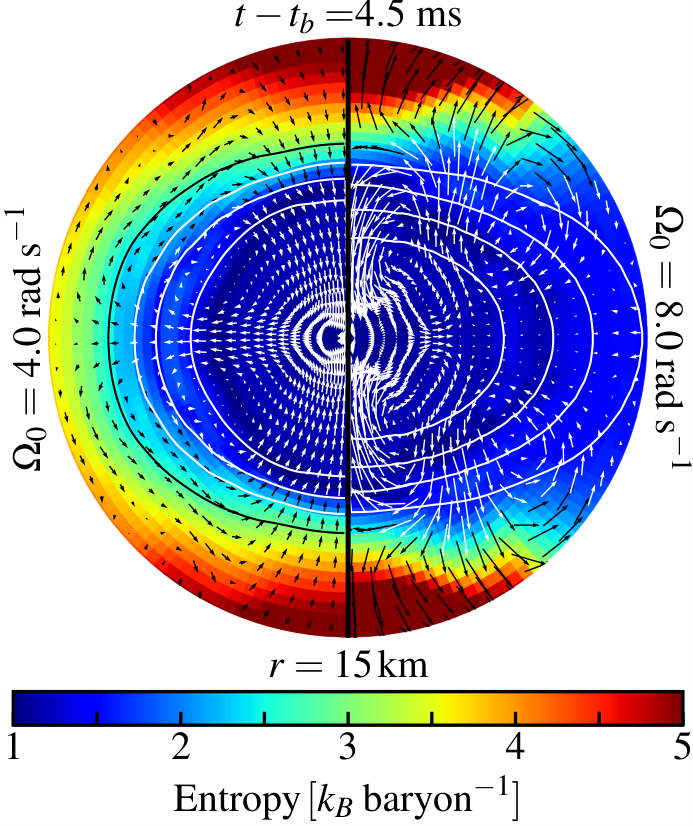
The bounce of the rotationally-deformed core excites postbounce “ring-down” oscillations of the PNS that are a complicated mixture of multiple modes. They last for a few cycles after bounce, are damped hydrodynamically [112], and cause the postbounce oscillations in the GW signal that are apparent in the left panel of Figure 4. The dominant oscillation has been identified as the (i.e., quadrupole) fundamental mode (i.e., no radial nodes) [55, 112]. The quadrupole oscillations can be seen in the postbounce velocity field that we plot in the left panel of Figure 5. With increasing rotation rate, changes in the mode structure and nonlinear coupling with other modes result in the complex flow geometries shown in the right panel of Figure 5. The density contours in Figure 5 also visualize how the PNS becomes more oblate and less dense with increasing rotation rate.
After the PNS has rung down, other fluid dynamics, notably prompt convection, begin to dominate the GW signal, generating a stochastic GW strain whose time domain evolution is sensitive to the perturbations from which prompt convection grows (e.g., [47, 46, 113, 57]). We exclude the convective part of the signal from our analysis. For our analysis, we delineate the end of the bounce signal and the start of the postbounce signal at , defined as the time of the third zero crossing of the GW strain. We also isolate the postbounce PNS oscillation signal from the convective signal by considering only the first after .
In the right panel of Figure 4, we show the Fourier transforms of each of the time-domain waveforms shown in the left panel, multiplied by for comparison with GW detector sensitivity curves. The bounce signal is visible in the broad bulge in the range of . The postbounce oscillations produce a peak in the spectrum of around , the center of which we call the peak frequency . Both the peak frequency and the amplitude of the bounce signal in general depend on both the rotation profile and the EOS.
IV.1 The Bounce Signal
The bounce spike is the loudest component of the GW signal. In Figure 6, we plot , the difference between the highest and lowest points in the bounce signal strain, as a function of the ratio of rotational kinetic energy to gravitational potential energy of the inner core at core bounce (see the beginning Section IV for details of our definition of core bounce). We assume a distance of and optimal detector orientation. Just as in Abdikamalov et al. [57], we see that at low rotation rates, the amplitude increases linearly with rotation rate, with a similar slope for all EOS. At higher rotation rates, the curves diverge from this linear relationship due to centrifugal support as the angular velocity at bounce approaches the Keplerian angular velocity. Rotation slows the collapse, softening the violent EOS-driven bounce and resulting in a smaller acceleration of the mass quadrupole moment. However, the value of at which simulations diverge from the linear relationship depends on the value of the differential rotation parameter . Stronger differential rotation affords less centrifugal support at higher rotation energies, allowing the linear behavior to survive to higher rotation rates.
The linear relationship between the bounce amplitude and of the inner core at bounce can be derived in a perturbative, order-of-magnitude sense. The GW amplitude depends on the second time derivative of the mass quadrupole moment , where is the mass of the oscillating inner core and and are the equatorial and polar equilibrium radii, respectively. If we treat the inner core as an oblate sphere, we can call the radius of the inner core in the polar direction and the larger radius of the inner core in the equatorial direction (due to centrifugal support) . To first order in , the mass quadrupole moment becomes
| (7) |
The difference between polar and equatorial radii in our simplified scenario can be determined by noting that the surface of a rotating sphere in equilibrium is an isopotential surface with a potential of , where is the distance to the rotation axis, is the distance to the origin, is the angular rotation rate, and is the gravitational constant. Setting the potential at the equator and poles equal to each other yields
| (8) |
Assuming differences between equatorial and polar radii are small, we can take only the terms to get . Solving for ,
| (9) |
The timescale of core bounce is the dynamical time . In this order-of-magnitude estimate we can replace time derivatives in Equation 6 with division by the dynamical time. We can also approximate . This results in
| (10) |
Though the mass and polar radius of the PNS depend on rotation as well, the dependence is much weaker (in the slow rotating limit) [57], and contains all of the first-order rotation effects used in the derivation. Hence, in the linear regime, the bounce signal amplitude should depend approximately linearly on , which is reflected by Figure 6.
| EOS | ||||
|---|---|---|---|---|
| BHBL | 318 | -0.03 | 321 | 0.598 |
| BHBLP | 317 | 0.02 | 322 | 0.599 |
| HSDD2 | 316 | 0.00 | 322 | 0.599 |
| SFHo | 306 | 0.03 | 304 | 0.582 |
| HSFSG | 306 | -0.00 | 325 | 0.602 |
| SFHx | 305 | 0.09 | 303 | 0.581 |
| HSIUF | 304 | 0.06 | 316 | 0.593 |
| HSNL3 | 298 | 0.07 | 324 | 0.600 |
| HSTMA | 295 | 0.15 | 315 | 0.593 |
| HSTM1 | 295 | 0.18 | 314 | 0.591 |
| HShenH | 281 | 0.28 | 311 | 0.604 |
| HShen | 280 | 0.29 | 310 | 0.604 |
| SFHo_ecap0.1 | 274 | 0.22 | 262 | 0.562 |
| GShenNL3 | 267 | 0.32 | 298 | 0.592 |
| GShenFSU1.7 | 264 | 0.24 | 294 | 0.587 |
| GShenFSU2.1 | 263 | 0.24 | 293 | 0.587 |
| LS180 | 242 | 0.16 | 245 | 0.536 |
| LS375 | 237 | 0.15 | 284 | 0.562 |
| LS220 | 237 | 0.20 | 258 | 0.543 |
| SFHo_ecap1.0 | 210 | 0.08 | 207 | 0.506 |
| SFHo_ecap10.0 | 174 | 0.03 | 198 | 0.482 |
Differences between EOS in the bounce signal enter through the mass and radius of the inner core at bounce (cf. Equation 10). Neither nor of the inner core are particularly well defined quantities since they vary rapidly around bounce – all quantitative results we state depend on our definition of the bounce time and Equation 10 is expected to be accurate only to an order of magnitude. With that in mind, in order to test how well Equation 10 matches our numerical results, we generate fits to functionals of the form . is simply the y-intercept of the line, which should be approximately 0 based on Equation 10. is the slope of the line, which we expect to be based on Equation 10, using the mass and radius of the nonrotating PNS at bounce. We include the arbitrary factor of 8 to make the order-of-magnitude predicted slopes similar to the fitted slopes. In Table 4 we show the results of the linear least-squares fits to results of slowly rotating collapse below for each EOS. Though is of the same order of magnitude as , significant differences exist. This is not unexpected, considering that our model does not account for nonuniform density distribution and the increase of the inner core mass with rotation, which can significantly affect the quadrupole moment.
At a given inner core mass, the structure (i.e. radius) of the inner core is determined by the EOS. Furthermore, the mass of the inner core is highly sensitive to the electron fraction in the final stages of collapse. In the simplest approximation, it scales with [114], which is due to the electron EOS that dominates until densities near nuclear density are reached. The inner-core in the final phase of collapse is set by the deleptonization history, which varies between EOS (Figure 3). In addition, contributions of the nonuniform nuclear matter EOS play an additional -independent role in setting . For example, we see from Figure 3 that the LS220 EOS yields a bounce of 0.278, while the GShenFSU2.1 EOS results in 0.267. Naively, relying just on the dependence of , we would expect LS220 to yield a larger inner core mass. Yet, the opposite is the case: our simulations show that the nonrotating inner core mass at bounce for the GShenFSU2.1 EOS is while that for the LS220 EOS is .
| Model | ||||
|---|---|---|---|---|
| [] | [] | [] | ||
| A32.5-LS220 | 3.976 | 0.020 | 0.589 | 4.7 |
| A32.5-SFHo | 4.262 | 0.020 | 0.624 | 6.1 |
| A32.5-SFHx | 4.252 | 0.020 | 0.610 | 6.1 |
| A32.5-GShenFSU2.1 | 3.612 | 0.020 | 0.634 | 5.2 |
| A32.5-HSDD2 | 3.582 | 0.019 | 0.629 | 5.9 |
| A32.5-BHB | 3.583 | 0.019 | 0.629 | 6.0 |
| A35.0-LS220 | 3.581 | 0.071 | 0.673 | 15.3 |
| A35.0-SFHo | 3.868 | 0.074 | 0.708 | 20.8 |
| A35.0-SFHx | 3.857 | 0.074 | 0.705 | 21.0 |
| A35.0-GShenFSU2.1 | 3.376 | 0.072 | 0.729 | 17.1 |
| A35.0-HSDD2 | 3.314 | 0.071 | 0.712 | 21.3 |
| A35.0-BHB | 3.321 | 0.071 | 0.709 | 21.3 |
| A37.5-LS220 | 2.940 | 0.141 | 0.784 | 15.5 |
| A37.5-SFHo | 3.183 | 0.146 | 0.829 | 16.1 |
| A37.5-SFHx | 3.237 | 0.147 | 0.831 | 16.0 |
| A37.5-GShenFSU2.1 | 2.878 | 0.143 | 0.838 | 17.3 |
| A37.5-HSDD2 | 2.763 | 0.142 | 0.835 | 17.1 |
| A37.5-BHB | 2.763 | 0.142 | 0.835 | 17.1 |
We further investigate the EOS-dependence of the bounce GW signal by considering a representative quantitative example of models with precollapse differential rotation parameter , computed with the six EOS identified in Section II as most compliant with constraints. In Table 5, we summarize the results for these models for three precollapse rotation rates, , probing different regions in Figure 6.
At , all models reach of , hence are in the linear regime where Equation 10 holds. The LS220 EOS model has the smallest inner core mass and results in the smallest bounce GW amplitude of all EOS (cf. also Figure 6). The SFHx and the GShenFSU2.1 EOS models have roughly the same inner core masses (), but the SFHx EOS is considerably softer, resulting in higher bounce density and correspondingly smaller radius, and thus larger , (at ) vs. for the GShenFSU2.1 EOS. We also note that the HSDD2 and the BHB EOS models give nearly identical results. They employ the same low-density EOS and the same RMF DD2 parameterization and their only difference is that includes softening hyperon contributions that appear above nuclear density. However, at the densities reached in our core collapse simulations with these EOS (), the hyperon fraction barely exceeds 1% [80] and thus has a negligible effect on dynamics and GW signal.
The models at listed in Table 5 reach and begin to deviate from the linear relationship of Equation 10. However, their bounce amplitudes still follow the same trends with EOS (and resulting inner core mass and bounce density) as their more slowly spinning counterparts.
Finally, the rapidly spinning models with listed in Table 5 result in and are far outside the linear regime. Centrifugal effects play an important role in their bounce dynamics, substantially decreasing their bounce densities and increasing their inner core masses. Increasing rotation, however, tends to decrease the EOS-dependent relative differences in . At , the standard deviation of is 12.5% of the mean value, while at , it is only 3%. This is also visualized by Figure 6 in which the rapidly rotating models cluster rather tightly around the A3 branch (third from the bottom). In general, for any value of , the EOS-dependent spread on a given differential rotation branch is smaller than the spread between branches.
Conclusions: In the Slow Rotation regime () the bounce GW amplitude varies linearly with (Equation 10), in agreement with previous works. Small differences in this linear slope are due primarily to differences in the inner core mass at bounce induced by different EOS. In the Rapid Rotation regime () the core is centrifugally supported at bounce and the bounce GW signal depends much more strongly on the amount of precollapse differential rotation than on the EOS. In the Extreme Rotation regime () the core undergoes a centrifugally-supported bounce and the GW bounce signal weakens.
IV.2 The Postbounce Signal from PNS Oscillations
The observable of greatest interest in the postbounce GW signal is the oscillation frequency of the PNS, which may encode EOS information. To isolate the PNS oscillation signal from the earlier bounce and the later convective contributions, we separately Fourier transform the GW signal calculated from GWs up to (the end of the bounce signal, defined as the third zero-crossing after core bounce as in Figure 4) and from GWs up to (empirically chosen to produce reliable PNS oscillation frequencies). We begin with a simulation with intermediate rotation and subtract the former bounce spectrum from the latter full spectrum and we take the largest spectral feature in the window of to to be the f-mode peak frequency [55, 112]. The spectral windows for simulations with the same value of and adjacent values of are centered at this frequency and have a width of . This process is repeated outward from the intermediate simulation and allows us to more accurately isolate the correct oscillation frequency in slowly and rapidly rotating regimes where picking out the correct spectral feature is difficult. This procedure is visualized in Figure 7. Note that there are only around five to ten postbounce oscillation cycles before the oscillations damp, so the peak has a finite width of about . However, our analysis in this section shows that the peak frequency is known far better than that.
In the top panel of Figure 8, we plot the GW peak frequency as a function of (of the inner core at bounce) for each of our 1704 collapsing cores. We identify three regimes of rotation and systematics in this figure:
(Slow Rotation Regime) In slowly rotating cores, , shows little variation with increasing rotation rate or degree of differential rotation. Note that our analysis is unreliable in the very slow rotation limit (). There, the PNS oscillations are only weakly excited and the corresponding GW signal is very weak. This is a consequence of the fact that our nonlinear hydrodynamics approach is noisy and not made for the perturbative regime.
(Rapid Rotation Regime) In the rapidly rotating regime, , increases with increasing rotation rate and initially more differentially rotating cores have systematically higher .
(Extreme Rotation Regime) At , bounce and the postbounce dynamics become centrifugally dominated, leading to very complex PNS oscillations involving multiple nonlinear modes with comparable amplitudes. This makes it difficult to unambiguously define in this regime and our analysis becomes unreliable. Excluding all models with leaves us with 1487 simulations with a reliable determination of .
Figure 8 shows that the different EOS lead to a variation in . The peak frequency is expected to scale with the PNS dynamical frequency (e.g., [112]). That is,
| (11) |
where is the gravitational constant and is the central density. In the bottom panel of Figure 8, we normalize the observed peak frequency by the dynamical frequency, using the central density averaged over after the end of the bounce signal (the same time interval from which we extract ). The scatter between different EOS is drastically reduced, and thus the effect of the EOS on the peak frequency is essentially parameterized by the PNS central density, which is a reflection of the compactness of the PNS core.
| EOS | |||||
|---|---|---|---|---|---|
| SFHo_ecap0.1 | 871 | 7.9 | 795 | 3.74 | 0.656 |
| SFHo_ecap1.0 | 846 | 9.4 | 778 | 3.58 | 0.573 |
| SFHo_ecap10.0 | 790 | 10.5 | 760 | 3.42 | 0.532 |
| SFHo | 772 | 5.6 | 784 | 3.64 | 0.650 |
| SFHx | 769 | 7.3 | 785 | 3.64 | 0.648 |
| LS180 | 727 | 7.4 | 767 | 3.48 | 0.611 |
| HSIUF | 725 | 8.6 | 747 | 3.30 | 0.656 |
| LS220 | 724 | 6.2 | 756 | 3.38 | 0.616 |
| GShenFSU2.1 | 723 | 10.9 | 734 | 3.19 | 0.664 |
| GShenFSU1.7 | 722 | 10.6 | 735 | 3.20 | 0.665 |
| LS375 | 709 | 8.0 | 729 | 3.15 | 0.626 |
| HSTMA | 704 | 5.6 | 702 | 2.91 | 0.661 |
| HSFSG | 702 | 7.6 | 731 | 3.16 | 0.662 |
| HSDD2 | 701 | 8.2 | 723 | 3.09 | 0.660 |
| BHB | 700 | 8.3 | 723 | 3.09 | 0.660 |
| BHB | 700 | 8.4 | 722 | 3.09 | 0.659 |
| GShenNL3 | 699 | 11.9 | 691 | 2.83 | 0.671 |
| HSTM1 | 675 | 5.1 | 688 | 2.80 | 0.659 |
| HShenH | 670 | 6.8 | 694 | 2.85 | 0.678 |
| HShen | 670 | 6.4 | 694 | 2.85 | 0.678 |
| HSNL3 | 669 | 3.8 | 681 | 2.75 | 0.660 |
In the Slow Rotation regime, the parameterization of with works particularly well, because centrifugal effects are mild and there is no dependence on the precollapse degree of differential rotation. In Table 6, we list and averaged over simulations with and broken down by EOS. We also provide the standard deviation for , average dynamical frequency, average time-averaged central density, and the average inner core mass at bounce for each EOS. These quantitative results further corroborate that and are closely linked. As expected from our analysis of the bounce signal in Section IV.1, hyperons have no effect: HShen and HShenH yield the same and and so do HSDD2, BHB, and BHB.
The results summarized by Table 6 also suggest that the subnuclear, nonuniform nuclear matter part of the EOS may play an important role in determining and PNS structure. This can be seen by comparing the results for EOS with the same high-density uniform matter EOS but different treatment of nonuniform nuclear matter. For example, GShenNL3 and HSNL3 both employ the RMF NL3 model for uniform matter, but differ in their descriptions of nonuniform matter (cf. Section II). They yield that differ by . Similarly, GShenFSU1.7 (and GShenFSU2.1) produce higher peak frequencies than HSFSG. Interestingly, the difference between HShen and HSTM1 (both using RMF TM1) in is much smaller even though they have substantially different averaged and .
Figure 8 shows that is roughly constant in the Slow Rotation regime, but increases with faster rotation in the Rapid Rotation regime. Centrifugal support, leads to a monotonic decrease of the PNS density with increasing rotation (cf. Figure 5). Thus, naively and based on Equation (11), we would expect a decrease with increasing rotation rate. We observe the opposite and this warrants further investigation.
Figure 8 also shows that in the Rapid Rotation regime the precollapse degree of differential rotation determines how quickly the peak frequency increases with , suggesting that may not be the best measure of rotation for the purposes of understanding the behavior of . Instead, in Figure 9, we plot the normalized peak frequency as a function of a different measure of rotation, (normalized by ), the highest equatorial angular rotation rate achieved at any time outside of a radius of . We impose this limit to prevent errors from dividing by small radii in . This is a convenient way to measure the rotation rate of the configuration without needing to refer to a specific location or time. This produces an interesting result (Figure 9): all our simulations for which we are able to reliably calculate the peak frequency follow the same relationship in which the normalized peak frequency is essentially independent of rotation at lower rotation rates (Slow Rotation), followed by a linear increase with rotation rate at higher rotation rates (Rapid Rotation). Note that the transition between these regimes and the two parts of Figure 9 occurs just when .
We can gain more insight into the relationship of and by considering Figure 10, in which we plot both (top panel) and (bottom panel) against the dynamical frequency . Since rotation decreases , rotation rate increases from right to left in the figure.
First, consider in the top panel of Figure 10. At high (Slow Rotation regime), all cluster with EOS below the line with small differences between rotation rates, just as we saw in Figures 8 and 9. However, as the rotation rate increases (and decreases), rapidly increases and exhibits the spreading with differential rotation already observed in Figure 8. Notably, this occurs in the region where the peak PNS oscillation frequency exceeds its dynamical frequency, .
Now turn to the – relationship plotted in the bottom panel of Figure 10. At the lowest rotation rates, this plot simply captures how varies between EOS. For slowly rotating cores, is substantially smaller than the dynamical frequency , and points cluster in a line for each EOS. As surpasses , this smoothly transitions to the Rapid Rotation regime, in which is significantly driven down with increasing rotation rate. At the highest rotation rates (Extreme Rotation regime), exceeds by a few times and centrifugal effects dominate in the final phase of core collapse, preventing further collapse and spin-up. Faster initial rotation (lower ) results in lower in this regime, consistent with previous work [57].
The bottom panel of Figure 10 also allows us to understand the effect of precollapse differential rotation. Stronger differential rotation naturally reduces centrifugal support. Thus it allows a collapsing core to reach higher before centrifugal forces prevent further spin-up. This causes the spreading branches for the different A values in our models.
Armed with the above observations on differential rotation and the – and – relationships, we now return to Figure 9. It depicts a sharp transition in the behavior of at . A sharp transition is present in the – relationship, but not in the – relationship shown in Figure 10. The variable connected to PNS structure, , instead varies smoothly and slowly with rotation through the line. This is a strong indication that the sharp upturn of at in Figure 9 is due to a change in the dominant PNS oscillation mode rather than due to an abrupt change in PNS structure. The observation that centrifugal effects do not become dominant until is several times corroborates this interpretation.
In Figure 11, we plot the GW signals along with the equatorial and polar radial velocities from the origin for all 20 simulations using the SFHo EOS with a differential rotation parameter . The postbounce GW frequency clearly follows the frequency of the fluid oscillations. Both frequencies begin to significantly increase at around (corresponding to , red-colored graphs). The polar and equatorial velocity oscillation amplitudes initially increase with rotation rate (colors going from blue to red), but when rotation becomes rapid (colors going from red to green) the equatorial velocities decrease and polar velocities continue to grow. This demonstrates that the multi-dimensional PNS mode structure is altered at rapid rotation and no longer follows a simple description. This is also apparent from comparing the left and right panels of Figure 5.
While the above results show that the increase in is most likely a consequence of changes in the mode structure with rotation, it is not obvious what detailed process is driving the changes. While future work will be needed to answer this conclusively, we can use the work of Dimmelmeier et al. [115] as the basis of educated speculation. They study oscillations of rotating equilibrium polytropes and show that the f-mode frequency has a weak dependence on both rotation rate and differential rotation. This is consistent with our findings for models in the Slow Rotation regime (). They also identify several inertial modes whose restoring force is the Coriolis force (e.g., [116]). The inertial mode frequency increases rapidly with rotation and is sensitive to differential rotation, which is what we see for our PNS oscillations in the Rapid Rotation regime (). Our PNS cores are also significantly less dense than the equilibrium models of [115], which allows the modes in our simulations to have lower oscillation frequencies that intersect with the frequencies of the inertial modes in [115]. It could thus be that in our PNS cores inertial and f-mode eigenfunctions overlap and couple nonlinearly, leading to an excitation of predominantly inertial oscillations as rotation becomes more rapid. The increase of the inertial mode frequency with rotation would explain the trends we see in in Figure 8.
Coriolis forces should become dynamically important for oscillations when the oscillation frequency is locally smaller than the Coriolis frequency, given by (e.g., [117]), where is the latitude from the equator and, for simplicity, is a uniform rotation rate. Thus, we expect Coriolis effects to become locally relevant when . The kink in Figure 9 is at , and hence the behavior of the PNS oscillations changes precisely when we expect Coriolis effects to begin to matter. This is supports the notion that the PNS oscillations may be transitioning to inertial nature at high rotation rates.
Conclusions: The effects of the EOS on the postbounce GW frequency can be parameterized almost entirely in terms of the dynamical frequency of the core after bounce. In the Slow Rotation regime (), the postbounce frequency depends little on rotation rate. In the Rapid Rotation regime (), inertial effects modify the nature of the oscillations, causing the frequency to increase with rotation rate. We find that the maximum rotation rate outside of is the most useful parameterization of rotation for the purpose of understanding the oscillation frequencies. In the Extreme Rotation regime (), the postbounce GW frequency decreases with rotation because centrifugal support keeps the core very extended.
IV.3 GW Correlations with Parameters and EOS
We are interested in how characteristics of the GWs vary with rotation, properties of the EOS, and the resulting conditions during core collapse and after bounce. Rather than plot every variable against each other variable, we employ a simple linear correlation analysis. We calculate a linear correlation coefficient between two quantities and that quantifies the strength of the linear relationship between two variables:
| (12) |
The summation is over all simulations included in the analysis. The sample standard deviation of a quantity is
| (13) |
where is the average value of over all simulations. The correlation coefficient is always bound between (strong negative correlation) and (strong positive correlation). This only accounts for linear correlations, so even if two variables are tightly coupled, nonlinear relationships will reduce the magnitude of the correlation coefficient and a more involved analysis would be necessary for characterizing nonlinear relationships (see, e.g., [56]).
We display the correlation coefficients of several relevant quantities in Figure 12. , , , , and are all innate properties of a given EOS (Section II). and are the input parameters that determine the rotation profile as defined in Equation 5. The rest of the quantities are outputs from the simulations. Quantities defined at the time of core bounce are the inner core mass , the central electron fraction , the inner core angular momentum , and the ratio of the inner core rotational energy to gravitational energy . Rotation is also parameterized by the maximum rotation rate and by (see Section IV.2 for definitions). GW characteristics are quantified in the amplitude of the bounce signal , the peak frequency of the postbounce signal , and its variant normalized by the dynamical frequency . The bottom left half of the plot shows the values of the correlation coefficients for 874 simulations in the Slow Rotation regime (, ) and the top right half shows correlations for 613 simulations in the Rapid Rotation regime (, ).
There is a region in the bottom right corner of Figure 12 that shows the correlations between EOS parameters , , , , and . Since we chose to use existing EOS rather than create a uniform parameter space, there are correlations between the input values of , , and that impose some selection bias on the other correlations. In our set of 18 EOS, there is a strong correlation between and both and . The maximum neutron star mass correlates most strongly with and . These findings are not new and just reflect current knowledge of how the nuclear EOS affects neutron star structure (e.g., [118, 22, 23]). The small amount of asymmetry in this corner is the effect of selection bias, as some EOS contribute more data points to one or the other rotation regime.
Next, we note that the central at bounce () exhibits correlations with EOS characteristics , , and . This encodes the EOS dependence in the high-density part of the trajectories shown in Figure 3. The mass of a nonrotating inner core at bounce is sensitive to (though we note that it is also sensitive to at lower densities and to EOS properties). Our linear analysis in Figure 12 picks this up as a clear correlation between and . This correlation is stronger in the slow to moderately rapidly rotating models (bottom left half of the figure) and weaker in the rapidly rotating models (top right half of the figure) since in these models rotation strongly increases . This can also be seen in the strong correlations of with all of the rotation variables.
As discussed in Section IV.1 and pointed out in previous work (e.g., [57]), the GW signal from bounce, quantified by , is very sensitive to mass and of inner core at bounce. Our correlation analysis confirms this and shows that the is also correlated equally strongly with and as with . As expected from Figure 6, correlation with the differential rotation parameter is weak in the slow to moderately rapid rotation regime, but there is a substantial anti-correlation with the value of in the rapidly rotating regime (the smaller , the more differentially spinning a core is at the onset of collapse).
Figure 12 also shows that the most interesting correlations of any observable from an EOS perspective are exhibited by the peak postbounce GW frequency . In the slow to moderately rapidly rotating regime (), has its strongest correlations with EOS characteristics , , , through their influence on the PNS central density and is essentially independent of the rotation rate (cf. Figures 8 and 9). For rapidly rotating models () there is instead a clear correlation of with all rotation quantities. Note that the correlations with EOS quantities are all but removed for the normalized peak frequency . This supports our claim in Section IV.2 that the influence of the EOS on the peak frequency is parameterized essentially by the postbounce dynamical frequency .
Conclusions: Linear correlation coefficients show the interdependence of rotation parameters, EOS parameters, and simulation results. We use these to support our claims that the EOS dependence is parameterized by the dynamical frequency and that rotation is dynamically important for oscillations in the Rapid Rotation regime.
IV.4 Prospects of Detection and Constraining the EOS
The signal to noise ratio (SNR) is a measure of the strength of a signal observed by a detector with a given level of noise. We calculate SNRs using the Advanced LIGO noise curve at design sensitivity in the high-power zero-detuning configuration [30, 108]. We assume optimistic conditions where the rotation axis is perpendicular to the line of sight and the LIGO interferometer arms are optimally oriented and from the core collapse event. Following [119, 57], we define the matched-filtering SNR of an observed GW signal as
| (14) |
where is observed data and is a template waveform. When we calculate an SNR for our simulated signals, we take to mimic the GWs from the source matching a template exactly, and this simplifies to . The inner product integrals are calculated using
| (15) |
where is the one-sided noise spectral density. We follow the LIGO convention [120] for Fourier transforms, namely
| (16) |
Furthermore, we estimate the difference between two waveforms as seen by Advanced LIGO with the mismatch described and implemented in Reisswig & Pollney [121]:
| (17) |
where the latter term is the match between the two waveforms and is maximized over the relative arrival times of the two waveforms . Note that due to the axisymmetric nature of our simulations, our waveforms only have the polarization, making a maximization over complex phase unnecessary.
The simulated waveforms span a finite time and is sampled at nonuniform intervals. To mimic real LIGO data, we resample the GW time series data at the LIGO sampling frequency of before performing the discrete Fourier transform.
In Figure 13, we show the SNR for our 1704 collapsing cores assuming a distance of to Earth. Faster rotation (higher of the inner core at bounce) leads to stronger quadrupolar deformations, in turn causing stronger signals that are more easily observed, but only up to a point. If rotation is too fast, centrifugal support keeps the core more extended with lower average densities, resulting in a less violent quadrupole oscillation and weaker GWs. This happens at lower rotation rates for the rotation profiles that are more uniformly rotating (e.g., the series), since the large amount of angular momentum and rotational kinetic energy created by even a small rotation rate can be enough to provide significant centrifugal support. The more strongly differentially rotating cases (e.g., the series) require much faster rotation before centrifugal support becomes important at bounce. This also means that they can reach greater inner core deformations and generate stronger GWs.
All of the EOS result in similar SNRs for a given rotation profile. We observe a larger spread with EOS in estimated SNR for the rapid, strongly differentially rotating cases. The bounce part is the strongest part of the GW signal and dominates the SNR. Hence, the EOS-dependent differences in the bounce signal pointed out in Section IV.1 are most relevant for understanding the EOS systematics seen in Figure 13. For example, the LS220 EOS yields the smallest inner core masses at bounce and correspondingly the smallest . This translates to the systematically lower SNRs for this EOS.
We can get a rough estimate for how different the waveforms are with the simple scalar mismatch (Equation 17), which we calculate with respect to the simulations using the SFHo EOS and the same value of and . Simulations using different EOS but the same initial rotation profile will result in slightly different values of at bounce, so this measures the difference between waveforms from the same initial conditions rather than from the same bounce conditions. In the context of a matched-filter search, the mismatch roughly represents the amount of SNR lost due to differences between the template and the signal. However, note that searches for core collapse signals in GW detector data have thus far relied on waveform-agnostic methods that search for excess power above the background noise (e.g., [122]).
Figure 14 shows the results of the mismatch calculations. The large mismatches at are simply due to the small amplitudes of the GWs causing large relative errors. The mismatch results for such slowly spinning models have no predictive power and we do not analyze them further. At higher rotation rates, the dynamics are increasingly determined by rotation and decreasingly determined by the details of the EOS, and the mismatch generally decreases with increasing rotation rate.
An exception to this rule occurs in the Extreme Rotation regime () where waveforms show increasing mismatches with SFHo simulation results (most notably, LS220 and LS180). In this regime, the bounce dynamics changes due to centrifugal support and bounce occurs below nuclear saturation density for some EOS. Moreover, when centrifugal effects become dominant, bounce is also slowed down, widening the GW signal from bounce and reducing its amplitude. The initial rotation rate around which this occurs differs between EOS and the resulting qualitative and quantitative changes in the waveforms drive the increasing mismatches.
In Figure 14, the HShen EOS (included in the gray crosses) consistently shows the highest mismatch with SFHo. These two EOS use different low-density and high-density treatments (see Table 1 and Section II). It is insightful to compare mismatches between EOS using the same (or similar) physics in either their high-density or low-density treatments of nuclear matter in order to isolate the origin of large mismatch values. In the following, we again use the example of the rotation profile and compute mismatches between pairs of EOS. HShen and HSTM1 both use the RMF TM1 parameterization for high-density uniform matter, but deal with nonuniform lower-density matter in different ways (see Section II). Their mismatch is . GShenNL3 and HSNL3 use the RMF NL3 parameterization for uniform matter and also differ in their nonuniform matter treatment. They have a mismatch of . This is comparable to the HShen-SFHo mismatch of . We find a mismatch of for the GShenFSU2.1–HSFSG pair. Both use the RMF FSUGold parameterization for uniform nuclear matter and again differ in the nonuniform parts.
The above results suggest that the treatment of low-density nonuniform nuclear matter is at least in some cases an important differentiator between EOS in the GW signal of rotating core collapse. While perhaps somewhat unexpected, this finding may, in fact, not be too surprising: Previous work (e.g., [44, 57]) already showed that the GW signal of rotating core collapse is sensitive to the inner core mass at bounce (and, of course, its , angular momentum, or its maximum angular velocity; cf. Section IV.3). The inner core mass at bounce is sensitive to the low-density EOS through the pressure and speed of sound in the inner core material in the final phase of collapse and through chemical potentials and composition, which determine electron capture rates and thus the in the final phase of collapse and at bounce.
We can also compare EOS with the same treatment of nonuniform lower-density matter, but different high-density treatments. We again pick the () model sequence as an example for quantitative differences. GShenFSU2.1 and GShenFSU1.7 () differ only at super-nuclear densities, where GShenFSU2.1 is extra stiff in order to support a neutron star. HShenH adds hyperons to HShen (), BHB adds hyperons to HSDD2 (), and BHB includes an extra hyperonic interaction over BHB (). All of the Hempel-based EOS (HS, SFH, BHB) use identical treatments of low-density nonuniform matter, but parameterize the EOS of uniform nuclear matter differently. For our example rotation profile, the mismatch with SFHo varies from 0.12% (for SFHx) to 7.6% (for GShenNL3). The results are comparable with the mismatch induced by differences in the low-density regime.
Conclusions: We expect a maximum SNR of around from a source at a distance of , though this depends both on the amount of differential rotation and the EOS. Using use a simple scalar mismatch to calculate the differences between waveforms generated using different EOS, we find that both the treatment of nonuniform and uniform nuclear matter significantly affect the waveforms, though differences at densities more than about twice nuclear are of little importance.
IV.5 Effects of Variations in Electron Capture Rates
Electron capture in the collapse phase is a crucial ingredient in CCSN simulations and influences the inner core mass at bounce () by setting the electron fraction in the final phase of collapse (e.g., [74, 123]). As pointed out in the literature (e.g., [61, 44, 55, 57]), and in this study (cf. Section IV.1), at bounce and after bounce has a decisive influence on the rotating core collapse GW signal.
In order to study how variations in electron capture rates affect our GW predictions, we carry out three additional sets of simulations using the SFHo EOS, , and all 20 corresponding values of listed in Table 2.
In one set of simulations, SFHo_ecap1.0, we employ a parameterization obtained from GR1D simulations using the approach of Sullivan et al. [73] that incorporates detailed tabulated electron capture rates for individual nuclei. This is an improvement over the prescriptions of [124, 125] that operates on an average nucleus. Sullivan et al. [73] found that randomly varying rates for individual nuclei has little effect, but systematically scaling rates by all nuclei with a global constant can have a large effect on the resulting deleptonization during collapse. In order to capture a factor in uncertainty, the other two additional sets of simulations use parameterizations, obtained by scaling the detailed electron capture rates by (SFHo_ecap0.1) and (SFHo_ecap10.0).
In Figure 15, we plot the three new profiles together with our fiducial SFHo profile. All of the new profiles predict substantially lower at high densities than our fiducial profiles for the SFHo EOS. However, the SFHo_ecap0.1 profile, and to a lesser extent the SFHo_ecap1.0 profile, have higher at intermediate densities of than the fiducial profile. This is relevant for our analysis here, since in the final phase of collapse, a large part of the inner core passes this density range less than a dynamical time from core bounce. Thus, the higher in this density range can have an influence on the inner core mass at bounce.
In the nonrotating case, the fiducial SFHo inner core mass at bounce is and we find , , and , for SFHo_0.1x_ecap, SFHo_1x_ecap, and SFHo_10x_ecap, respectively. Note that SFHo_1x_ecap and SFHo_10x_ecap give the same at , but SFHo_1x_ecap predicts higher at (cf. Figure 15) and thus has a larger inner core mass at bounce.
In Figure 16, we present the key GW observables and resulting from our rotating core collapse simulations with the new profiles. We also plot our fiducial SFHo results for comparison. The top panel shows and we note that the differences between the fiducial SFHo simulations and the runs with the SFHo_ecap1.0 base profile are substantial and larger than differences between many of the EOS discussed in Section IV.1 (cf. Figure 6). The differences with SFHo_ecap10.0 are even larger. The SFHo_ecap0.1 simulations produce that are very close to the fiducial SFHo results in the Slow Rotation regime. This is a consequence of the fact that the inner core masses of the fiducial SFHo and SFHo_ecap0.1 simulations are very similar in this regime (cf. Section IV.1). SFHo_ecap1.0 and SFHo_ecap10.0 produce smaller , because their inner cores are less massive at bounce.
The bottom panel of Figure 16 shows , the peak frequencies of the GWs from postbounce PNS oscillations. Again, there are large differences in between the fiducial SFHo simulations and those using obtained from detailed nuclear electron capture rates. These differences are as large as the differences between many of the EOS shown in Figure 8. In the Slow Rotation regime and into the Rapid Rotation regime, the SFHo_ecap1.0 base simulations have that are systematically higher than the fiducial SFHo simulations. For the SFHo_ecap0.1 the difference is and in the SFHo_ecap10.0 case, the difference is surprisingly only .
For the SFHo_ecap0.1 runs, we find a higher time-averaged postbounce central density than in the fiducial case. Hence, the higher we observe fits our expectations from Section IV.2. Explaining differences for SFHo_ecap1.0 and SFHo_ecap10.0 is more challenging: We find that SFHo_ecap1.0 runs have that are similar or slightly lower than those of the fiducial SFHo simulations, yet SFHo_ecap1.0 are systematically higher. Similarly, SFHo_ecap10.0 are systematically lower than the fiducial , yet the predicted are about the same. These findings suggest that not only , but also other factors, e.g., possibly the details for the distribution in the inner core or the immediate postbounce accretion rate play a role in setting .
As a quantitative example, we choose the previously considered case and compare our fiducial results with those of the detailed electron capture runs. For the fiducial SFHo run, we find (at ) and , with and . The corresponding detailed electron capture runs yield , , , and for SFHo_ecap{0.1, 1.0, 10.0}, respectively. The differences between these fiducial and detailed electron capture runs are comparable to the differences between the fiducial SFHo EOS and the fiducial LS220 EOS simulations discussed in Sections IV.1 and IV.2.
When considering the GW mismatch for the case between fiducial SFHo, and SFHo_ecap0.1, SFHo_ecap1.0, and SFHo_ecap10.0, we find we find 6.2%, 6.2%, and 4.9%, respectively. These values are larger than the mismatch values due to EOS differences shown in Figure 14.
Conclusions: The results of this exercise clearly show that the GW signal is very sensitive to the treatment of electron capture during collapse. Differences in this treatment and in capture rates can blur differences between EOS. Though a systematic uncertainty in electron capture rates by a factor as large as 10 in either direction is unlikely, the differences caused by variations in described in this section are major issues if one seeks to extract EOS information from an observed rotating core collapse GW signal.
V Conclusions
We carried out more than 1800 two-dimensional rapidly rotating general-relativistic hydrodynamic core collapse simulations to investigate the effects the nuclear EOS has on GW signals from rapidly rotating stellar core collapse, using 18 microphysical EOS and 98 different rotation profiles.
We distinguish three rotation regimes based on the ratio of rotational kinetic to gravitational energy of the inner core at bounce: Slow Rotation (), Rapid Rotation (), and Extreme Rotation (). We find that in the Slow Rotation regime, the behavior of the GW bounce signal is nearly independent of the EOS and is straightforwardly explained by an order of magnitude perturbative analysis. The amplitude of the bounce signal varies linearly with the rotation rate, parameterized by of the inner core at bounce, in agreement with previous work (e.g., [57, 44]). The differences between bounce signals from different EOS are due largely to corresponding differences in the mass of the inner core at bounce. The GWs from postbounce oscillations of the protoneutron star are almost independent of the rotation rate in the Slow Rotation regime. The effects of the EOS on the GW frequency can be parameterized almost entirely in terms of the dynamical frequency of the core after bounce.
In the Rapid Rotation regime, the maximum rotation rate at bounce exceeds the dynamical frequency (above ), and inertial (i.e. Coriolis and centrifugal forces) effects become significant and fundamentally change the character of the oscillations. The bounce amplitudes depart from their linear relationship with and depend on both the EOS and the degree of precollapse differential rotation. The variations due to the EOS are significantly smaller than those due to differing rotation profiles. Inertial effects confine oscillations to the poles and increase the oscillation frequency approximately linearly with the maximum rotation rate. Even in this regime, the dynamical time of the postbounce core parameterizes the effects of the EOS on top of the effects of rotation.
In the Extreme Rotation regime () the stellar cores undergo a centrifugally-supported bounce. Increasing the rotation rate in this regime leads to smaller rotational kinetic energy at bounce as centrifugal support keeps the collapsed cores more extended. The bounce GW signal correspondingly weakens, and the postbounce GW frequency appears to decrease, though weaker protoneutron star oscillations make positively identifying the peak frequency less reliable.
Our results show that EOS differences in the collapse phase are as important as the high-density parameterization in determining characteristics of the GWs. Different treatments of low-density matter produce differences in the bounce signal, postbounce oscillation frequency, and overall signal (as measured by the GW mismatch) that are comparable to those produced by differences in high-density parameterizations or differences in the treatment of the transition from nonuniform to uniform nuclear matter. Densities do not exceed around twice nuclear density in the bounce and brief postbounce phases of core collapse that we study. Hence, the GW signal from these phases does not probe exotic physics or conditions in very massive neutron stars.
We demonstrate that using detailed electron capture rates for individual nuclei as opposed to the fiducial single nucleus approach to electron capture results in differences in the bounce and postbounce GWs comparable to those caused by using a different EOS. The GW characteristics are also sensitive to systematic uncertainties in the electron capture rates, producing similarly large variations when scaling the capture rates by a factor of 10 in either direction. We also demonstrate that a density-parameterization of the electron fraction during the collapse phase lacks the precision required for detailed interpretation of observed GW signals. Variations in the way the parameterization is implemented produce changes in the GWs comparable to those produced by different EOS. This leads us to the conclusion that for quantitatively reliable GW predictions full multi-dimensional neutrino radiation-hydrodynamic simulations that include realistic weak interactions will be needed.
In Figure 17, we plot the GW bounce signal amplitude against the frequency of GWs from postbounce oscillations to show that different EOS occupy different, though partially overlapping regions in this observable space. This effectively maps uncertainties in the nuclear EOS to uncertainties in predicted GW signals from rapidly-rotating core collapse. Signals observed from the bounce and early postbounce phases of rotating core collapse outside of this region would be of great interest, since they would indicate unanticipated EOS physics and/or collapse dynamics. It may be possible to use the bounce amplitude to determine how quickly the star is rotating at bounce. The peak frequency could then constrain the EOS if there is enough core rotation to produce a reliable postbounce oscillation peak and little enough for the collapse to be in the Slow Rotation regime.
However, we must note that there are large uncertainties in the measured distances and orientations of nearby core-collapse supernovae, and also in the errors introduced by approximations made in the simulations. GW strain decreases inversely with distance, so the bounce amplitude is known only as well as the distance. Since the observed GW strain varies roughly with , where is the angle between the rotation axis and the line of sight, an accurate determination of the source orientation is required to be able to map the GW strain to a rotation rate. Inferring the peak frequency does not require distance or orientation measurements, but is subject to other observational uncertainties, e.g., the GW detector phase accuracy. Parameter estimation and model selection studies with more sophisticated data analysis tools, like those used by [57, 45, 126], are required to evaluate the feasibility of extracting EOS properties given real detector characteristics and noise.
It should also be noted that GWs from rotating core collapse will only be detectable from sources out to the Magellanic Clouds. Furthermore, even those cores that are in our Slow Rotation regime are still very rapidly spinning from a stellar evolution point of view and produce protoneutron stars with spin periods of . Massive stars with rapidly spinning cores are expected to be exceedingly rare. These caveats and the above limitations, combined with the relatively small differences in the GW characteristics and protoneutron star oscillations induced by EOS variations, mean that we are unlikely to be able to use a GW signal from rotating core collapse to discern the EOS with current GW detectors and simulation methods.
The present study has elucidated the various ways in which the nuclear EOS can impact the rotating core collapse GW signal. While we are confident that our qualitative findings are robust, our GW signal predictions are not quantitatively reliable. The most important limitation to be removed by future work is the lack of 2D neutrino radiation-hydrodynamics in the collapse phase. Our results on differences caused by differing treatments of various regimes of the same underlying EOS parameterization also suggest that more work in nuclear theory may be needed. In particular, there is an important need for consistent EOS frameworks with which only differences in EOS physics, but not differences in methods, cause differences in the GW signal. In addition, though previous studies have shown that different progenitors result in only slightly different inner core masses [127] and GW signal characteristics (assuming the same resulting inner core mass and angular momentum) [55], a quantitative understanding of progenitor-induced uncertainties will require a much more exhaustive study of progenitor dependence of GW signals from rotating CCSNe.
While axisymmetry is a good approximation for collapse, bounce, and the early postbounce phase ( after bounce), rotating core collapse is host to rich three dimensional (3D) postbounce dynamics that can drive GW emission, including rotational instabilities and the nonaxisymmetric standing accretion shock instability. 3D simulations of rotating core collapse and postbounce GW emission have been carried out (e.g., [49, 128, 129]), but the EOS dependence of the GWs generated by 3D dynamics has yet to be explored. GWs from prompt and neutrino-driven convection and from the standing accretion shock instability in both rotating and nonrotating core collapse [130, 131, 132] have some EOS dependence as well [46, kuroda:16b], but the EOS parameter space has thus far been only sparsely sampled. Future studies of GWs emitted by these dynamics may yet provide alternate means of discerning the nuclear EOS.
acknowledgements
We would like to thank Jim Fuller, Hannah Klion, Peter Goldreich, Hiroki Nagakura, Pablo Cerdá-Durán, Hajime Sotani, Luke Roberts, André da Silva Schneider, Chuck Horowitz, Jim Lattimer, Sarah Gossan, and Bill Engels for many insightful discussions. The authors wish to thank Remco Zegers for supporting the development of the (EC) weak rate library, which was instrumental in the completion of this work. SR was supported by the DOE CSGF, which is provided under grant number DE-FG02-97ER25308, and the NSF Blue Waters Graduate Fellowship. This research is part of the Blue Waters sustained-petascale computing project, which is supported by the National Science Foundation (awards OCI-0725070 and ACI-1238993) and the State of Illinois. Blue Waters is a joint effort of the University of Illinois at Urbana-Champaign and its National Center for Supercomputing Applications. These simulations were performed on the Stampede cluster of the NSF XSEDE network under allocation TG-PHY100033 and benefited from access to Blue Waters under allocation NSF PRAC ACI-1440083. This research is supported by the NSF under award numbers CAREER PHY-1151197, AST-1212170, and PHY-1404569, by the International Research Unit of Advanced Future Studies, Kyoto university, and by the Sherman Fairchild Foundation. EA acknowledges support from NU ORAU and Social Policy grants. CS acknowledges support from the National Science Foundation under grant No. PHY-1430152 (JINA Center for the Evolution of the Elements) and No. PHY-1102511 and from the Department of Energy National Nuclear Security Administration under award number DE-NA0000979. EO acknowledges support for this work by NASA through Hubble Fellowship grant #51344.001-A awarded by the Space Telescope Science Institute, which is operated by the Association of Universities for Research in Astronomy, Inc., for NASA, under contract NAS 5-26555.
References
- [1] H. A. Bethe, Rev. Mod. Phys. 62, 801 (1990).
- [2] H. A. Bethe and J. R. Wilson, Astrophys. J. 295, 14 (1985).
- [3] S. M. Couch and C. D. Ott, Astrophys. J. 799, 5 (2015).
- [4] S. W. Bruenn, E. J. Lentz, W. R. Hix, A. Mezzacappa, J. A. Harris, O. E. B. Messer, E. Endeve, J. M. Blondin, M. A. Chertkow, E. J. Lingerfelt, et al., Astrophys. J. 818, 123 (2016).
- [5] J. M. LeBlanc and J. R. Wilson, Astrophys. J. 161, 541 (1970).
- [6] G. S. Bisnovatyi-Kogan, Astron. Zh. 47, 813 (1970).
- [7] A. Burrows, L. Dessart, E. Livne, C. D. Ott, and J. Murphy, Astrophys. J. 664, 416 (2007).
- [8] T. Takiwaki, K. Kotake, and K. Sato, Astrophys. J. 691, 1360 (2009).
- [9] S. G. Moiseenko, G. S. Bisnovatyi-Kogan, and N. V. Ardeljan, Mon. Not. Roy. Astron. Soc. 370, 501 (2006).
- [10] P. Mösta, S. Richers, C. D. Ott, R. Haas, A. L. Piro, K. Boydstun, E. Abdikamalov, C. Reisswig, and E. Schnetter, Astrophys. J. Lett. 785, L29 (2014).
- [11] N. Smith, W. Li, A. V. Filippenko, and R. Chornock, Mon. Not. Roy. Astron. Soc. 412, 1522 (2011).
- [12] J. Hjorth and J. S. Bloom, in Chapter 9 in ”Gamma-Ray Bursts”, Cambridge Astrophysics Series 51, eds. C. Kouveliotou, R. A. M. J. Wijers and S. Woosley, Cambridge University Press (Cambridge) (2012), pp. 169–190.
- [13] M. Modjaz, Astron. Nachr. 332, 434 (2011).
- [14] M.-A. Dupret, K. Belkacem, R. Samadi, J. Montalban, O. Moreira, A. Miglio, M. Godart, P. Ventura, H.-G. Ludwig, A. Grigahcène, et al., Astron. Astrophys. 506, 57 (2009).
- [15] A. Heger, S. E. Woosley, and H. C. Spruit, Astrophys. J. 626, 350 (2005).
- [16] C. D. Ott, A. Burrows, T. A. Thompson, E. Livne, and R. Walder, Astrophys. J. Suppl. Ser. 164, 130 (2006).
- [17] J. Fuller, M. Cantiello, D. Lecoanet, and E. Quataert, Astrophys. J. 810, 101 (2015a).
- [18] S. E. Woosley and A. Heger, Astrophys. J. 637, 914 (2006).
- [19] S.-C. Yoon, N. Langer, and C. Norman, Astron. Astrophys. 460, 199 (2006).
- [20] S. E. de Mink, N. Langer, R. G. Izzard, H. Sana, and A. de Koter, Astrophys. J. 764, 166 (2013).
- [21] C. L. Fryer and A. Heger, Astrophys. J. 623, 302 (2005).
- [22] J. M. Lattimer, Ann. Rev. Nuc. Part. Sc. 62, 485 (2012).
- [23] M. Oertel, M. Hempel, T. Klähn, and S. Typel, arXiv:1610.03661 (2016).
- [24] K. Hebeler, J. M. Lattimer, C. J. Pethick, and A. Schwenk, Phys. Rev. Lett. 105, 161102 (2010).
- [25] K. Hebeler, J. M. Lattimer, C. J. Pethick, and A. Schwenk, Astrophys. J. 773, 11 (2013).
- [26] E. E. Kolomeitsev, J. M. Lattimer, A. Ohnishi, and I. Tews, Submitted to Phys. Rev. Lett. ; arXiv:1611.07133 (2016).
- [27] J. Nättilä, A. W. Steiner, J. J. E. Kajava, V. F. Suleimanov, and J. Poutanen, Astron. Astrophys. 591, A25 (2016).
- [28] F. Özel and P. Freire, Ann. Rev. Astron. Astrophys. 54, 401 (2016).
- [29] B. P. Abbott et al. (LIGO Scientific Collaboration, Virgo Collaboration), Phys. Rev. Lett. 116, 061102 (2016a).
- [30] J. Aasi et al. (LIGO Scientific Collaboration), Class. Quantum Grav. 32, 074001 (2015).
- [31] K. Somiya (for the KAGRA collaboration), Class. Quantum Grav. 29, 124007 (2012).
- [32] F. Acernese et al. (Virgo Collaboration), Tech. Rep. VIR-027A-09, Virgo Collaboration (2009), URL https://tds.ego-gw.it/itf/tds/file.php?callFile=VIR-0027A-09.pdf.
- [33] S. Bernuzzi, A. Nagar, M. Thierfelder, and B. Bruegmann, Phys. Rev. D 86, 044030 (2012).
- [34] S. Bernuzzi, T. Dietrich, and A. Nagar, Phys. Rev. Lett. 115, 091101 (2015).
- [35] É. É. Flanagan and T. Hinderer, Phys. Rev. D 77, 021502 (2008).
- [36] J. S. Read, C. Markakis, M. Shibata, K. Uryū, J. D. E. Creighton, and J. L. Friedman, Phys. Rev. D 79, 124033 (2009).
- [37] M. Vallisneri, Phys. Rev. Lett. 84, 3519 (2000).
- [38] M. Shibata and K. Taniguchi, Phys. Rev. D 77, 084015 (2008).
- [39] D. Radice, S. Bernuzzi, W. Del Pozzo, L. F. Roberts, and C. D. Ott, Submitted to Phys. Rev. Lett.; arXiv:1612.06429 (2016).
- [40] S. Bernuzzi, D. Radice, C. D. Ott, L. F. Roberts, P. Mösta, and F. Galeazzi, Phys. Rev. D 94, 024023 (2016).
- [41] N. Stergioulas, A. Bauswein, K. Zagkouris, and H.-T. Janka, Mon. Not. Roy. Astron. Soc. 418, 427 (2011).
- [42] A. Bauswein and H.-T. Janka, Phys. Rev. Lett. 108, 011101 (2012).
- [43] A. Bauswein, N. Stergioulas, and H.-T. Janka, Phys. Rev. D 90, 023002 (2014).
- [44] H. Dimmelmeier, C. D. Ott, A. Marek, and H.-T. Janka, Phys. Rev. D 78, 064056 (2008).
- [45] C. Röver, M. Bizouard, N. Christensen, H. Dimmelmeier, I. S. Heng, and R. Meyer, Phys. Rev. D 80, 102004 (2009).
- [46] A. Marek, H.-T. Janka, and E. Müller, Astron. Astrophys. 496, 475 (2009).
- [47] C. D. Ott, Class. Quantum Grav. 26, 063001 (2009).
- [48] K. Kotake, Comptes Rendus Physique 14, 318 (2013).
- [49] C. D. Ott, H. Dimmelmeier, A. Marek, H.-T. Janka, I. Hawke, B. Zink, and E. Schnetter, Phys. Rev. Lett. 98, 261101 (2007a).
- [50] C. D. Ott, H. Dimmelmeier, A. Marek, H.-T. Janka, B. Zink, I. Hawke, and E. Schnetter, Class. Quantum Grav. 24, 139 (2007b).
- [51] C. L. Fryer and A. Heger, Astrophys. J. 541, 1033 (2000).
- [52] T. Takiwaki and K. Kotake, Astrophys. J. 743, 30 (2011).
- [53] P. Mösta, C. D. Ott, D. Radice, L. F. Roberts, R. Haas, and E. Schnetter, Nature 528, 376 (2015).
- [54] M. Obergaulinger, M. A. Aloy, and E. Müller, Astron. Astrophys. 450, 1107 (2006).
- [55] C. D. Ott, E. Abdikamalov, E. O’Connor, C. Reisswig, R. Haas, P. Kalmus, S. Drasco, A. Burrows, and E. Schnetter, Phys. Rev. D 86, 024026 (2012).
- [56] W. J. Engels, R. Frey, and C. D. Ott, Phys. Rev. D 90, 124026 (2014).
- [57] E. Abdikamalov, S. Gossan, A. M. DeMaio, and C. D. Ott, Phys. Rev. D 90, 044001 (2014).
- [58] S. E. Gossan, P. Sutton, A. Stuver, M. Zanolin, K. Gill, and C. D. Ott, Phys. Rev. D 93, 042002 (2016).
- [59] E. Müller, Astron. Astrophys. 114, 53 (1982).
- [60] T. Zwerger and E. Müller, Astron. Astrophys. 320, 209 (1997).
- [61] R. Mönchmeyer, G. Schäfer, E. Müller, and R. Kates, Astron. Astrophys. 246, 417 (1991).
- [62] S. Yamada and K. Sato, Astrophys. J. 450, 245 (1995).
- [63] K. Kotake, S. Yamada, and K. Sato, Phys. Rev. D 68, 044023 (2003).
- [64] C. D. Ott, A. Burrows, E. Livne, and R. Walder, Astrophys. J. 600, 834 (2004).
- [65] H. Dimmelmeier, J. A. Font, and E. Müller, Astron. Astrophys. 393, 523 (2002).
- [66] H. Dimmelmeier, C. D. Ott, H.-T. Janka, A. Marek, and E. Müller, Phys. Rev. Lett. 98, 251101 (2007).
- [67] J. M. Lattimer and F. D. Swesty, Nucl. Phys. A 535, 331 (1991).
- [68] Lattimer-Swesty EOS Webpage, http://www.astro.sunysb.edu/dswesty/lseos.html.
- [69] H. Shen, H. Toki, K. Oyamatsu, and K. Sumiyoshi, Nucl. Phys. A 637, 435 (1998a).
- [70] H. Shen, H. Toki, K. Oyamatsu, and K. Sumiyoshi, Prog. Th. Phys. 100, 1013 (1998b).
- [71] H. Shen, H. Toki, K. Oyamatsu, and K. Sumiyoshi, Astrophys. J. Suppl. Ser. 197, 20 (2011a).
- [72] H. Shen et al. EOS Tables, http://user.numazu-ct.ac.jp/~sumi/eos/.
- [73] C. Sullivan, E. O’Connor, R. G. T. Zegers, T. Grubb, and S. M. Austin, Astrophys. J. 816, 44 (2016).
- [74] W. R. Hix, O. E. B. Messer, A. Mezzacappa, M. Liebendörfer, J. Sampaio, K. Langanke, D. J. Dean, and G. Martínez-Pinedo, Phys. Rev. Lett. 91, 201102 (2003).
- [75] G. Shen, C. J. Horowitz, and S. Teige, Phys. Rev. C 83, 035802 (2011b).
- [76] G. Shen, C. J. Horowitz, and E. O’Connor, Phys. Rev. C 83, 065808 (2011c).
- [77] M. Hempel and J. Schaffner-Bielich, Nuc. Phys. A 837, 210 (2010).
- [78] M. Hempel, T. Fischer, J. Schaffner-Bielich, and M. Liebendörfer, Astrophys. J. 748, 70 (2012).
- [79] A. W. Steiner, M. Hempel, and T. Fischer, Astrophys. J. 774, 17 (2013a).
- [80] S. Banik, M. Hempel, and D. Bandyopadhyay, Astrophys. J. Suppl. Ser. 214, 22 (2014).
- [81] J. M. Lattimer, C. J. Pethick, D. G. Ravenhall, and D. Q. Lamb, Nuc. Phys. A 432, 646 (1985).
- [82] C. F. v. Weizsäcker, Zeitschrift für Physik 96, 431 (1935).
- [83] H. A. Bethe and R. F. Bacher, Rev. Mod. Phys. 8, 82 (1936).
- [84] J. Piekarewicz, Journal of Physics G Nuclear Physics 37, 064038 (2010).
- [85] M. B. Tsang, Y. Zhang, P. Danielewicz, M. Famiano, Z. Li, W. G. Lynch, and A. W. Steiner, Phys. Rev. Lett. 102, 122701 (2009).
- [86] A. Carbone, G. Colò, A. Bracco, L.-G. Cao, P. F. Bortignon, F. Camera, and O. Wieland, Phys. Rev. C 81, 041301 (2010).
- [87] L. Chen, Science China Physics, Mechanics, and Astronomy 54, 124 (2011).
- [88] J. Antoniadis, P. C. C. Freire, N. Wex, T. M. Tauris, R. S. Lynch, M. H. van Kerkwijk, M. Kramer, C. Bassa, V. S. Dhillon, T. Driebe, et al., Science 340, 448 (2013).
- [89] Equation of state tables by Matthias Hempel, http://phys-merger.physik.unibas.ch/~hempel/eos.html.
- [90] Equation of state tables by Gang Shen, http://cecelia.physics.indiana.edu/gang_shen_eos/.
- [91] G. Shen, C. J. Horowitz, and S. Teige, Phys. Rev. C 82, 015806 (2010a).
- [92] G. Shen, C. J. Horowitz, and S. Teige, Phys. Rev. C 82, 045802 (2010b).
- [93] S. Gandolfi, J. Carlson, and S. Reddy, Phys. Rev. C 85, 032801 (2012).
- [94] A. W. Steiner, J. M. Lattimer, and E. F. Brown, Astrophys. J. Lett. 765, L5 (2013b).
- [95] A. W. Steiner, S. Gandolfi, F. J. Fattoyev, and W. G. Newton, Phys. Rev. C 91, 015804 (2015).
- [96] F. Özel, D. Psaltis, T. Güver, G. Baym, C. Heinke, and S. Guillot, Astrophys. J. 820, 28 (2016).
- [97] M. C. Miller and F. K. Lamb, Eur. Phys. J. A 52, 63 (2016).
- [98] S. Guillot and R. E. Rutledge, Astrophys. J. Lett. 796, L3 (2014).
- [99] M. Liebendörfer, Astrophys. J. 633, 1042 (2005).
- [100] E. B. Abdikamalov, C. D. Ott, L. Rezzolla, L. Dessart, H. Dimmelmeier, A. Marek, and H. Janka, Phys. Rev. D 81, 044012 (2010).
- [101] S. E. Woosley and A. Heger, Phys. Rep. 442, 269 (2007).
- [102] E. O’Connor, Astrophys. J. Suppl. Ser. 219, 24 (2015).
- [103] E. J. Lentz, A. Mezzacappa, O. E. B. Messer, W. R. Hix, and S. W. Bruenn, Astrophys. J. 760, 94 (2012).
- [104] H. Dimmelmeier, J. Novak, J. A. Font, J. M. Ibáñez, and E. Müller, Phys. Rev. D 71, 064023 (2005).
- [105] J. A. Font, Liv. Rev. Rel. 11, 7 (2008).
- [106] P. Colella and P. R. Woodward, J. Comp. Phys. 54, 174 (1984).
- [107] B. Einfeldt, SIAM Journal on Numerical Analysis 25, 294 (1988).
- [108] D. Shoemaker, Tech. Rep. LIGO-T0900288-v3, LIGO Scientific Collaboration (2010), URL https://dcc.ligo.org/LIGO-T0900288/public.
- [109] KAGRA Detector Sensitivity, URL http://gwcenter.icrr.u-tokyo.ac.jp/researcher/parameters.
- [110] L. S. Finn and C. R. Evans, Astrophys. J. 351, 588 (1990).
- [111] L. Blanchet, T. Damour, and G. Schaefer, Mon. Not. Roy. Astron. Soc. 242, 289 (1990).
- [112] J. Fuller, H. Klion, E. Abdikamalov, and C. D. Ott, Mon. Not. Roy. Astron. Soc. 450, 414 (2015b).
- [113] K. Kotake, W. Iwakami, N. Ohnishi, and S. Yamada, Astrophys. J. Lett. 697, L133 (2009).
- [114] A. Yahil, Astrophys. J. 265, 1047 (1983).
- [115] H. Dimmelmeier, N. Stergioulas, and J. A. Font, Mon. Not. Roy. Astron. Soc. 368, 1609 (2006).
- [116] N. Stergioulas, Liv. Rev. Rel. 6, 3 (2003).
- [117] H. Saio, Prospects for Asteroseismology of Rapidly Rotating B-Type Stars (Springer Berlin Heidelberg, Berlin, Heidelberg, 2013), pp. 159–176, ISBN 978-3-642-33380-4, URL http://dx.doi.org/10.1007/978-3-642-33380-4_8.
- [118] J. M. Lattimer and M. Prakash, Astrophys. J. 550, 426 (2001).
- [119] É. É. Flanagan and S. A. Hughes, Phys. Rev. D 57, 4535 (1998).
- [120] S. Anderson, W. Anderson, K. Blackburn, P. Brady, D. Brown, P. Charlton, J. Creighton, T. Creighton, S. Finn, J. Romano, et al., Tech. Rep. LIGO-T010095-00-Z (2004), URL {https://dcc.ligo.org/LIGO-T010095/public}.
- [121] C. Reisswig and D. Pollney, Class. Quantum Grav. 28, 195015 (2011).
- [122] B. P. Abbott, R. Abbott, T. D. Abbott, M. R. Abernathy, F. Acernese, K. Ackley, C. Adams, T. Adams, P. Addesso, R. X. Adhikari, et al., ArXiv e-prints (2016b).
- [123] A. Burrows and J. M. Lattimer, Astrophys. J. 270, 735 (1983).
- [124] S. W. Bruenn, Astrophys. J. Suppl. Ser. 58, 771 (1985).
- [125] K. Langanke, G. Martínez-Pinedo, J. M. Sampaio, D. J. Dean, W. R. Hix, O. E. Messer, A. Mezzacappa, M. Liebendörfer, H.-T. Janka, and M. Rampp, Phys. Rev. Lett. 90, 241102 (2003).
- [126] J. Logue, C. D. Ott, I. S. Heng, P. Kalmus, and J. Scargill, Phys. Rev. D 86, 044023 (2012).
- [127] H.-T. Janka, F. Hanke, L. Hüdepohl, A. Marek, B. Müller, and M. Obergaulinger, Prog. Th. Exp. Phys. 2012, 01A309 (2012).
- [128] S. Scheidegger, S. C. Whitehouse, R. Käppeli, and M. Liebendörfer, Class. Quantum Grav. 27, 114101 (2010).
- [129] T. Kuroda, T. Takiwaki, and K. Kotake, Phys. Rev. D 89, 044011 (2014).
- [130] B. Müller, H.-T. Janka, and A. Marek, Astrophys. J. 766, 43 (2013).
- [131] K. N. Yakunin, A. Mezzacappa, P. Marronetti, S. Yoshida, S. W. Bruenn, W. R. Hix, E. J. Lentz, O. E. B. Messer, J. A. Harris, E. Endeve, et al., submitted to Phys. Rev. D, arXiv:1505.05824 (2015).
- [132] H. Andresen, B. Müller, E. Müller, and H.-T. Janka, ArXiv e-prints (2016).
- [133] E. O’Connor and C. D. Ott, Class. Quantum Grav. 27, 114103 (2010).
- [134] T. A. Thompson, E. Quataert, and A. Burrows, Astrophys. J. 620, 861 (2005).
Appendix A Fits
In the simulations presented in the main body of the paper we use and interpolate profiles directly from a 1D simulation snapshot. A commonly used alternative is to fit a function to this profile and evaluate the function rather than interpolating data in a profile. For convenience and for use in the numerics study in Appendix B, we also generate functional fits for these profiles. Following [99] with a tweak at high densities, we fit our 1D profiles using the fitting function
| (18) |
The parameters and are fixed. The parameters are fit using the Mathematica MyFit function, subject to the constraints
| (19) | ||||
| EOS | |||||
|---|---|---|---|---|---|
| SFHo | 7.795 | 12.816 | 0.308 | 0.0412 | 0.257 |
| SFHx | 7.767 | 12.633 | 0.323 | 0.0380 | 0.275 |
| SFHo_ecap0.1 | 8.210 | 13.053 | 0.291 | 0.0493 | 0.237 |
| SFHo_ecap1.0 | 8.022 | 12.882 | 0.281 | 0.0528 | 0.224 |
| SFHo_ecap10.0 | 7.743 | 12.405 | 0.294 | 0.0473 | 0.226 |
| LS180 | 7.738 | 13.034 | 0.290 | 0.0307 | 0.243 |
| LS220 | 7.737 | 12.996 | 0.292 | 0.0298 | 0.245 |
| LS375 | 7.755 | 12.901 | 0.295 | 0.0279 | 0.251 |
| HShen | 7.754 | 13.124 | 0.303 | 0.0398 | 0.267 |
| HShenH | 7.751 | 13.124 | 0.303 | 0.0397 | 0.267 |
| GShenFSU1.7 | 7.939 | 12.935 | 0.305 | 0.0403 | 0.257 |
| GShenFSU2.1 | 7.939 | 12.935 | 0.305 | 0.0403 | 0.257 |
| GShenNL3 | 7.917 | 13.104 | 0.299 | 0.0412 | 0.247 |
| HSDD2 | 7.797 | 12.813 | 0.308 | 0.0411 | 0.259 |
| HSNL3 | 7.798 | 12.808 | 0.308 | 0.0409 | 0.253 |
| HSIUF | 7.792 | 12.777 | 0.311 | 0.0403 | 0.257 |
| HSTMA | 7.793 | 12.787 | 0.310 | 0.0408 | 0.252 |
| HSTM1 | 7.799 | 12.812 | 0.308 | 0.0411 | 0.253 |
| HSFSG | 7.792 | 12.784 | 0.311 | 0.0404 | 0.256 |
| BHB | 7.794 | 12.815 | 0.308 | 0.0412 | 0.259 |
| BHB | 7.794 | 12.814 | 0.308 | 0.0412 | 0.259 |
| Liebendörfer G15 | 7.477 | 13.301 | 0.278 | 0.0350 | 0.278 |
The resulting fit parameters are listed in Table 7 for each EOS. In Figure 18, we plot the profiles for the SFHo EOS that we use in the SFHo 2D simulations, along with our fit. We also plot the G15 fit from [99], and the profile obtained by tracking the density and electron fraction of the center during collapse in the GR1D simulation and appending this to the at profile for low densities. We describe the results of test simulations using each of these profiles in Appendix B.
Appendix B Numerics Study
We attempt to quantify the errors resulting from the various numerical and physical approximations in our approach by performing a sensitivity study with various parameters in all simulation phases. We employ the SFHo EOS for these tests and adopt , as the fiducial rotation setup in rotating test simulations. Key quantitative results from the fiducial 1D and 2D simulations used for comparison are listed in bold at the top of Tables 8 and 9.
B.1 1D Tests
| Test | |||||
|---|---|---|---|---|---|
| GR1D Nonrot. | 180 | 0.583 | 4.31 | 14.9 | 0.288 |
| CoCoNuT Nonrot. | 174 | 0.582 | 4.38 | 14.8 | 0.278 |
| CoCoNuT Fiducial | 200 | 0.708 | 4.16 | 12.8 | 0.278 |
| GR1D | 180 | 0.583 | 4.26 | 14.9 | 0.288 |
| GR1D Rotating | 202 | 0.674 | 3.95 | 13.9 | 0.286 |
| GR1D Direct | 210 | 0.583 | 4.37 | 14.1 | 0.278 |
| GR1D Fit | 211 | 0.592 | 4.43 | 14.2 | 0.265 |
| GR1D Center | 174 | 0.610 | 4.26 | 17.3 | 0.279 |
| GR1D G15 | 189 | 0.547 | 4.22 | 12.5 | 0.279 |
| NuLib | 180 | 0.582 | 4.25 | 15.0 | 0.288 |
| NuLib | 180 | 0.583 | 4.27 | 14.7 | 0.288 |
| NuLib | 180 | 0.582 | 4.25 | 14.9 | 0.288 |
| NuLib | 180 | 0.583 | 4.28 | 14.8 | 0.288 |
As described in Section III, we use GR1D simulations to generate profiles for the 2D simulations, and so these profiles encode the effects of the EOS during the collapse phase of the 2D simulations. Here we check the various levels of physical and numerical approximations made in calculating the profiles used in the main text. We also check whether using one of these profiles produces results consistent with full transport. In Table 8, we list the time to bounce , the mass of the inner core at bounce , and the central density, temperature, and electron fraction at bounce.
Table 8 shows that the nonrotating 1D GR1D radiation-hydrodynamic simulation and the 2D CoCoNuT hydrodynamic simulation agree well in key collapse results and in particular in . This confirms that the parameterization captures deleptonization and its effect on the collapsing core well, as previously shown by [99]. The difference in the central at bounce ( in the GR1D run vs. in the CoCoNuT simulation) is due to our use of from the GR1D simulation at the time of minimum central , which occurs just before bounce. Due to shifts in the local beta equilibrium, the central in the radiations-hydrodynamic simulation increases again after its global minimum.
An important open question is to what extent rotation affects the validity of the for deleptonization during collapse. While we cannot currently carry out detailed multi-D radiation-hydrodynamic simulations to answer this conclusively, we can include rotation approximately in GR1D 1D radiation-hydrodynamic simulations, using the “shellular rotation” approximation (cf. [133, 134]). We employ the fiducial rotation profile specified by and as in the 2D case, though the radial coordinate relevant for the rotational setup is the spherical radius in GR1D.
The “GR1D Rotating” row in Table 8 shows that the effects of rotation on the collapse dynamics are qualitatively similar between 1D “shellular rotation” and 2D rotation: and increase and decreases. However, in 1D, the quantitative changes are smaller than in 2D, which is consistent with the findings of [16], who more extensively compared 1D “shellular rotation” with 2D rotation.
Figure 18 compares the profile obtained from the rotating GR1D simulation with the fiducial profile and other possible profiles. As expected (cf. Section III), rotation in the “shellular” approximation leads to only minor differences in between the nonrotating case and the fiducial rotational setup.
In the first row of the GR1D block of Table 8, we list results from a GR1D simulation with 1.5 times the standard resolution. The differences with the standard resolution run are very small, giving us confidence that ours GR1D simulation results are numerically converged.
The profiles extracted from the 1D radiation-hydrodynamic simulations should give a good approximation to collapse-phase deleptonization and its impact on collapse and bounce dynamics [99]. We test this assertion by re-running the GR1D 1D simulations with various choices for the profiles (see Figure 18) rather than using neutrino transport. The results are listed in the third block of Table 8.
We find that our fiducial profile (cf. Section III.1, row “GR1D Direct” in Table 8) leads to inner core masses, bounce densities, and thermodynamics that approximate the radiation hydrodynamics results very well. Using a fit to the fiducial (“GR1D Fit”) or generating the profile from the central value of (“GR1D Center”) leads to larger differences in all quantities (e.g., in ). These quantitative differences are of the same order as those due to differences in EOS and electron capture treatment (cf. Section IV.5 and the “GR1D G15” row). For instance, different EOS lead to inner core masses at bounce in the range of . Hence, the parameterization can lead to a systematic error that muddles the interpretation of results from simulations using different EOS. For quantitatively reliable predictions, full 2D radiation-hydrodynamic simulations will be necessary.
The entries in the NuLib block of Table 8 give results for test simulations with different resolutions of our neutrino interaction table. These are to be compared with the fiducial neutrino interaction table that has resolution (number of energy groups), , , . All tables span the range
| (20) | |||||
The energy, density, and temperature points in the table are logarithmically spaced and the electron fraction points are evenly spaced. Increasing the table resolution has negligible impact on the GR1D results.
B.2 2D Tests
| Test | ||||
| CoCoNuT Fiducial | 0.718 | 0 | 793 | 20.9 |
| NuLib | 0.717 | 2.10(-5) | 794 | 20.9 |
| NuLib | 0.718 | 2.91(-5) | 794 | 21.0 |
| NuLib | 0.717 | 4.63(-5) | 794 | 21.0 |
| NuLib | 0.718 | 1.48(-5) | 794 | 20.9 |
| GR1D | 0.716 | 1.23(-5) | 794 | 21.0 |
| GR1D Rotating | 0.711 | 9.21(-5) | 794 | 20.6 |
| Fit | 0.729 | 9.53(-3) | 812 | 20.6 |
| Center | 0.747 | 4.87(-2) | 810 | 23.3 |
| G15 | 0.655 | 7.86(-2) | 752 | 14.1 |
| CoCoNuT | 0.718 | 1.79(-3) | 795 | 21.5 |
| CoCoNuT | 0.718 | 1.03(-4) | 794 | 21.1 |
| CoCoNuT Eq. Bounce | 0.714 | 4.40(-3) | 789 | 21.6 |
| CoCoNuT rk3 | 0.716 | 3.34(-3) | 797 | 20.9 |
In Table 9, we list the inner core mass at bounce, the GW mismatch (see Section IV.4) with the fiducial 2D simulation, the peak frequency, and the bounce signal amplitude for several 2D tests. The results of the fiducial 2D simulation are bolded at the top for comparison.
The NuLib and GR1D blocks of Table 9 use the profile generated by the corresponding 1D test simulation in a 2D simulation otherwise identical to the fiducial one. These all produce negligible differences in all quantities. Rotation is multidimensional, so the “shellular rotation” approximation in GR1D does not take into account multidimensional effects. The lack of impact of approximate 1.5D rotation on the collapse deleptonization suggests that using a profile from a nonrotating 1D simulation in moderately-rapidly rotating 2D collapse simulation is acceptable. The choice of parameterization, however, leads to significant differences, as already pointed out in the previous Appendix B.1. The GW mismatch for the “Fit” and “Center” choices with the fiducial approach is 1% and 5%, respectively. The peak frequencies differ by 2%. Using the G15 fit of [99] leads to even larger mismatch of and a peak frequency differing by as much as . These differences are as large or larger than differences between many EOS discussed in §IV. We do not expect this to affect the universal trends we establish in the main text, since differences in EOS already produce different profiles yielding simulation results that consistently follow the universal trends. However, it reaffirms that for quantitatively reliable GW signal predictions, a detailed and converged treatment of prebounce deleptonization with radiation hydrodynamics is vital.
In the final block of Table 9, we summarize results of simulations in which we increase the resolution and order of the time integrator in CoCoNuT simulations. These lead to waveform mismatches of up to 0.4%, significantly smaller than those from systematic errors induced by the prebounce deleptonization treatment. As pointed out in Section III.2, we transition from the deleptonization prescription to neutrino leakage when the entropy along the polar axis exceeds . In rotating models, this is a fraction of a millisecond before this occurs on the equatorial axis, which is our definition of the time of core bounce. The row labeled “CoCoNuT Eq. Bounce” shows that having the trigger on the equatorial axis results in negligible differences.
To summarize, our 1D and 2D simulation results are essentially independent of the neutrino interaction table resolution and of the 1D grid resolution. There is a weak dependence on the 2D grid resolution (below 1% mismatch in all resolution tests). However, the results are sensitive to the treatment of prebounce deleptonization at the level of several percent GW mismatch. Again, future GR radiation hydrodynamic simulations with detailed nuclear electron capture rates will be needed for reliable predictions of gravitational waveforms from rotating core collapse.