Visualizing Residual Networks

In 2015, deep residual networks won 1st place on the ILSVRC classification task [3]. We seek to understand the qualitative characteristics underlying the shortcut connections and identity mappings that motivated He et al. towards this network architecture. To this end, we implement two visualizations of the feature maps after each residual building block: the top-9 images that maximally activate a unit in a given channel, and a guided backpropagation [6] visualization that unit’s activation.

From these visualizations, we can visually confirm He et al.’s intuition that preconditioning layers to the identity mapping helps, and that it is easier to learn functions relative to the identity mapping. Specifically, we observe that residual layers of the same dimensionality learn features that get refined and sharpened.

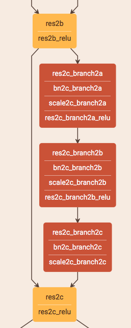
The CNN architecture that we used was a pretrained 50-layer residual network [3]. A visualization of the architecture can be found online (http://ethereon.github.io/netscope/#/gist/db945b393d40bfa26006) [1]. This residual architecture consists of a single convolution layer (conv1), then a max-pooling layer, then a series of residual shortcut building blocks. There are two flavors of residual shortcut block, both shown in figure 1. The first flavor consists of 1x1, 3x3, and 1x1 convolutional layers, with a shortcut adding the inputs to the 1x1 convolution to the outputs of the final 1x1 convolution, performed elementwise. This conditions the stack of 3 layers towards the identity mapping.

The second flavor is called a projection shortcut. It consists of the same stack of convolutional layers, except the shortcut now contains a single 1x1 convolution.

The 50-layer residual architecture consists of an initial preojection block (2a), followed by two basic blocks (2b, 2c). This is followed by a projection block (3a), and a series of basic blocks (3b, 3c). This basic pattern is repeated twice more (4a, then 4b, 4c, 4d, 4e, 4f. Also: 5a then 5b, 5c).

Two more differences are associated with the projection shortcut: reduced spatial dimension due to a stride of 2, and an increase in the number of channels. This means that building blocks named with the same number (e.g. 2a, 2b and 2c) contain the same number of output channels.

For our visualizations, we used code from Yosinski et al., modifying it to work with residual networks and modifying it to implement guided backpropagation instead of deconvolution [7].

To obtain the top-9 images maximally activating each unit, we used the ImageNet validation set. The units that are visualized are those with the highest activation values, across spatial dimensions, and across all images in the dataset. This means the visualization for a given filter is that of a specific spatial unit (e.g. position [20, 31] in the feature map for the channel).

To visualize the activation of this maximal unit, the image is fed through to the unit’s layer, all the other activations in that layer are zeroed out, and that layer is then passed backwards using guided backpropagation. When visualizing the top-9 images, we select the patch corresponding to the receptive field of the unit.

In figures 3 and  3, we have visualizations of channels across the 2a, 2b, and 2c building blocks (res2a, res2b, res2c). Filter 12 appears to recognize complex lined patterns, becoming more discriminative in res2b, and slightly more discriminative in res2c. Filter 79 does not appear to change substantially, which is consistent with the intuition that residual blocks are preconditioned to the identity mapping. Filter 150 exhibits refinement: at res2a, it recognizes slightly curved dark lines, but at res2b and res2c begins to recognize loops and tighter curves. Filter 210 does not appear to recognize anything in res2a, but shifts to recognize parallel lines in res2b and res2c.

In figure 4, we selected an interesting example of refinement of features. In res3a, it recognizes a single spot of light. In res3b, it is refined to recognize the spot of light with a surrounding context, and further in res3c.

In figures 6 and  6 we randomly chose 4 different filters to visualize. All exhibit the refinement effect. Filter 7 appears to recognize men in suits: initially 2 out of the top-9 activations are not of men in suits, but at res5c all are. Examining the deconvolution visualization confirms that this feature is not necessarily focusing on recognizing weddings: it appears the unit fixates on suit collars. Filter 149 recognizes a mosaic pattern, with little apparent refinement. Filter 1068 appears to recognize truss structures, initially containing a perfume bottle in its top activations, before later being dominated by satellite dishes and cranes. Filter 1620 initially highly activates on horned animals, with these activations being refined away by res5c.

In figure 7, we also selected another interesting example of refinement of object recognition. Channel 1660 in res5a has 1 tandem bicycle in its top-9 activations. In res5b, the same channel is maximally activated by 6 tandem bicycles, and by the final residual block of that feature size, res5c, all of the top-9 inputs are tandem bicycles. We speculate that the filters in the branches (e.g. res5b_branch2c and res5c_branch2c), focus on specific sub-features that help improve the detection of the feature. We see that res5b_branch2c (channel 1660) latches onto bikes with two seats and res5c_branch2c (channel 1660) activates on the spokes.

To see the benefits of ResNet’s architecture, we briefly examined AlexNet. AlexNet does not have these identity mappings, so to find units on different layers that correspond we compared the top-9 activation inputs from AlexNet conv4 to those of conv5. The units which matched on more than 1 input in common were few, and there were few examples of refinement as clear as in the residual network.

In figure 8 we also directly visualized the kernels in conv1 and found they were similar to AlexNet.

Several ideas came up during the course of this project that were not pursued due to time and compute constraints. These present interesting avenues for exploration:

1. 1.

   We did not examine the 1x1, 3x3, and 1x1 convolutions inside each residual block (e.g. inside res2a). These are particularly interesting because the first 1x1 convolution downsamples the channels, the 3x3 convolution maintains the channel dimensionality, and the final 1x1 convolution upsamples (e.g. 1024 channels $\rightarrow$ 256 channels $\rightarrow$ 256 channels $\rightarrow$ 1024 channels). It would be interesting to visualize these branched, additive, features.

2. 2.

   Across res* boundaries (e.g. res3c $\rightarrow$ res4a) the number of channels doubles and a projection building block is used (e.g. res4a). We did not visualize differences across these boundaries because there are no obvious correspondences between filters (unlike with the residual shortcuts). In other words, channel 60 in res4f does not map to channel 60 in res5a It would be interesting to find those correspondences and visualize the evolution of higher-level concepts. Some preliminary exploration found that a feature in the previous layer (e.g. res4f) would usually have more than one corresponding feature (sharing multiple top-9 activation patches) in the next layer (e.g. res5a), and those corresponding features would subsequently diverge.

3. 3.

   In the past several months, He et al. have made several improvements to the architecture of residual networks [4]. We could qualitatively evaluate those improvements.

4. 4.

   Having seen the refinement effect of these residual shortcuts, we could try exploiting this property to expand existing architectures. We speculate it would be possible to take a pretrained 7-layer AlexNet architecture, insert 0-initialized residual blocks of the same channel dimensionality before and after each pretrained layer, and then resume training.

References

- [1] Saumitro Dasgupta. Netscope.
- [2] Vincent Dumoulin and Francesco Visin. A guide to convolution arithmetic for deep learning. arXiv preprint arXiv:1603.07285, 2016.
- [3] Kaiming He, Xiangyu Zhang, Shaoqing Ren, and Jian Sun. Deep residual learning for image recognition. arXiv preprint arXiv:1512.03385, 2015.
- [4] Kaiming He, Xiangyu Zhang, Shaoqing Ren, and Jian Sun. Identity mappings in deep residual networks. arXiv preprint arXiv:1603.05027, 2016.
- [5] Alex Krizhevsky, Ilya Sutskever, and Geoffrey E. Hinton. Imagenet classification with deep convolutional neural networks. In Advances in Neural Information Processing Systems 25. 2012.
- [6] Jost Tobias Springenberg, Alexey Dosovitskiy, Thomas Brox, and Martin A. Riedmiller. Striving for simplicity: The all convolutional net. arXiv preprint arXiv:1412.6806, abs/1412.6806, 2014.
- [7] Jason Yosinski, Jeff Clune, Anh Nguyen, Thomas Fuchs, and Hod Lipson. Understanding neural networks through deep visualization. In Deep Learning Workshop, International Conference on Machine Learning (ICML), 2015.
- [8] Matthew D. Zeiler and Rob Fergus. Visualizing and understanding convolutional networks. In Proceedings of the European Conference on Computer Vision (ECCV), 2014.