Sliding-Window Superposition Coding:
Two-User Interference Channels

For high data rates and massive connectivity, next-generation cellular networks are expected to deploy many small base stations. While such dense deployment provides the benefit of bringing radio closer to end users, it also increases the amount of interference from neighboring cells. Consequently, efficient and effective management of interference is expected to become one of the main challenges for high-spectral-efficiency, low-power, broad-coverage wireless communications.

Over the past few decades, several techniques at different protocol layers [1, 2, 3] have been proposed to mitigate adverse effects of interference in wireless networks. One important conceptual technique at the physical layer is simultaneous decoding [4, Section 6.2], [5]. In this decoding method, each receiver attempts to recover both the intended and a subset of the interfering codewords at the same time. When the interference is strong [6, 7] and weak [8, 9, 10, 11], simultaneous decoding of random code ensembles achieves the capacity of the two-user interference channel. In fact, for any given random code ensemble, simultaneous decoding achieves the same rates achievable by the optimal maximum likelihood decoding [10, 12, 13]. The celebrated Han–Kobayashi coding scheme [14] also relies on simultaneous decoding as a crucial component. As a main drawback, however, each receiver in simultaneous decoding (or maximum likelihood decoding) has to employ some form of multiuser sequence detection, which usually has high computational complexity. This issue has been tackled recently by a few approaches based on emerging spatially coupled and polar codes [15, 16], but these solutions involve very long block lengths.

For this reason, most practical communication systems use conventional point-to-point low-complexity decoding. The simplest method is treating interference as noise, in which only statistical properties (such as the distribution and power), rather than the actual codebook information, of the interfering signals, are used. In successive cancellation decoding, similar low-complexity point-to-point decoding is performed in steps, first recovering interfering codewords and then incorporating them as part of the channel output for decoding of desired codewords. Successive cancellation decoding is particularly well suited when the messages are split into multiple parts by rate splitting, encoded into separate codewords, and transmitted via superposition coding. In particular, when there is only one receiver (i.e., for a multiple access channel), this rate-splitting coding scheme with successive cancellation decoding was proposed by Rimoldi and Urbanke [17] for the Gaussian case and Grant, Rimoldi, Urbanke, and Whiting [18] for the discrete case, and achieves the optimal rate region of the polymatroidal shape (the pentagon for two senders). When there are two or more receivers—as in the two-user interference channel or the compound multiple access channel—the rate-splitting multiple access scheme fails to achieve the optimal rate region as demonstrated earlier in [19] for Gaussian codes and in Section III-B of this paper (and [20]) for general codes.

A natural question is whether low-complexity point-to-point coding techniques, which could achieve capacity for multiple access and single-antenna Gaussian broadcast channels, are fundamentally deficient for the interference channel, and high-complexity simultaneous decoding would be critical to achieve the capacity in general. In this paper, we develop a new coding scheme, called sliding-window superposition coding, that overcomes the limitations of low-complexity decoding through a new diagonal superposition structure. The main ingredients of the scheme are block Markov coding, sliding-window decoding (both commonly used for multihop relaying and feedback communication), superposition coding, and successive cancellation decoding (crucial for low-complexity implementation using standard point-to-point codes). Each message is encoded into a single long codeword that are transmitted diagonally over multiple blocks and multiple signal layers, which helps avoid the performance bottleneck for the aforementioned rate-splitting multiple access scheme. Receivers recover the desired and interfering codewords over a decoding window spanning multiple blocks. Successive cancellation decoding is performed within each decoding window as well as across a sequence of decoding windows for streams of messages. When the number and distribution of signal layers are properly chosen, the sliding-window superposition coding scheme can achieve every rate pair in the rate region of maximum likelihood decoding for the two-user interference channel with single streams, providing a constructive answer to our earlier question. We develop a more complete theory behind the number and distribution of signal layers and the choice of decoding orders, which leads to an extension of this coding scheme that achieves the entire Han–Kobayashi inner bound.

For practical communication systems, the conceptual sliding-window superposition coding scheme can be readily adapted to a coded modulation scheme using binary codes and common signal constellations. We compare this sliding-window coded modulation scheme with two well-known coded modulation schemes, multi-level coding [21, 22] and bit-interleaved coded modulation [23, 24]. We implement the sliding-window coded modulation scheme for the two-user Gaussian channel using the 4G LTE turbo code and demonstrate its performance improvement over treating interference as noise. Following earlier conference versions [20, 25] of this paper, several practical implementations of sliding-window superposition coding have been investigated [26, 27] and proposed to the 5G standards [28, 29, 30, 31, 32, 33].

The rest of the paper is organized as follows. We first define the problem and the relevant rate regions in Section II. Then, we explain the rate-splitting scheme and demonstrate its fundamental deficiency for the interference channel in Section III. We introduce the new sliding-window superposition coding in Section IV, first by developing a simple scheme that achieves the corner points of simultaneous decoding region, and then extending it to achieve every point in the region. We devote Section V to sliding-window coded modulation and its application in a practical communication setting. In Section VI, we present a more complete theory of the sliding-window superposition coding scheme with a discussion on the number of superposition layers and alternative decoding orders. With further extensions and augmentations, we develop a scheme that achieves the Han–Kobayashi inner bound [14] for the two-user interference channel with point-to-point encoders and decoders in Section VII. We offer a couple of concluding remarks in Section VIII.

Throughout the paper, we closely follow the notation in [4]. In particular, for $X\sim p(x)$ and $\epsilon\in(0,1)$, we define the set of $\epsilon$-typical $n$-sequences $x^{n}$ (or the typical set in short) [34] as

We use $X_{k}^{n}$ to denote the vector $(X_{k1},X_{k2},\ldots,X_{kn})$. For $n=1,2,\ldots,[n]=\{1,2,\ldots,n\}$ and for $a\geq 0,[2^{a}]=\{1,2,\ldots,2^{\left\lceil a\right\rceil}\}$, where $\left\lceil a\right\rceil$ is the smallest integer greater than or equal to $a$. The probability of an event $\mathcal{A}$ is denoted by $\P(\mathcal{A})$.

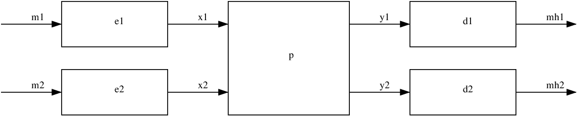
Consider the communication system model depicted in Fig. 1, whereby senders 1 and 2 wish to communicate independent messages $M_{1}$ and $M_{2}$ to their respective receivers over a shared channel $p(y_{1},y_{2}\mathchoice{\mspace{1mu}\mspace{1mu}}{}{}{}x,w)$. Here $X$ and $W$ are channel inputs from senders 1 and 2, respectively, and $Y_{1}$ and $Y_{2}$ are channel outputs at receivers 1 and 2, respectively. In network information theory, this model is commonly referred to as the two-user interference channel.

The Gaussian interference channel in Fig. 2 is an important special case with channel outputs

where $g_{jk}$ denotes the channel gain coefficient from sender $k$ to receiver $j$, and $N_{1}$ and $N_{2}$ are independent $\mathrm{N}(0,1)$ noise components. Under the average power constraint $P$ on each input $X$ and $W$, we denote the received signal-to-noise ratios (SNRs) as $S_{1}=g_{11}^{2}P$ and $S_{2}=g_{22}^{2}P$, and the received interference-to-noise ratios (INRs) as $I_{1}=g_{12}^{2}P$ and $I_{2}=g_{21}^{2}P$.

A $(2^{nR_{1}},2^{nR_{2}},n)$ code $\mathcal{C}_{n}$ for the (two-user) interference channel consists of

• $\bullet$

  two message sets $[2^{nR_{1}}]\mathchar 58\relax=\{1,\ldots,2^{\lceil nR_{1}\rceil}\}$ and $[2^{nR_{2}}]$,

• $\bullet$

  two encoders, where encoder 1 assigns a codeword $x^{n}(m_{1})$ to each message $m_{1}\in[2^{nR_{1}}]$ and encoder 2 assigns a codeword $w^{n}(m_{2})$ to each message $m_{2}\in[2^{nR_{2}}]$, and

• $\bullet$

  two decoders, where decoder 1 assigns an estimate ${\hat{m}}_{1}$ or an error message $\mathrm{e}$ to each received sequence $y_{1}^{n}$ and decoder 2 assigns an estimate ${\hat{m}}_{2}$ or an error message $\mathrm{e}$ to each received sequence $y^{n}_{2}$.

The performance of a given code $\mathcal{C}_{n}$ for the interference channel is measured by its average probability of error

where the message pair $(M_{1},M_{2})$ is uniformly distributed over $[2^{nR_{1}}]\times[2^{nR_{2}}]$. A rate pair $(R_{1},R_{2})$ is said to be achievable if there exists a sequence of $(2^{nR_{1}},2^{nR_{2}},n)$ codes $(\mathcal{C}_{n})_{n=1}^{\infty}$ such that $\lim_{n\to\infty}{P_{e}^{(n)}}(\mathcal{C}_{n})=0$. A set of rate pairs, typically referred to as a rate region, is said to be achievable if every rate pair in the interior of the set is achievable. The capacity region is the closure of the set of achievable rate pairs $(R_{1},R_{2})$, which is the largest achievable rate region and captures the optimal tradeoff between the two rates of reliable communication over the interference channel. The capacity region for the two-user interference channel is not known in general.

Let $p=p(x)p(w)$ be a given product pmf on $\mathcal{X}\times\mathcal{W}$. Suppose that the codewords $x^{n}(m_{1}),m_{1}\in[2^{nR_{1}}]$, and $w^{n}(m_{2}),m_{2}\in[2^{nR_{2}}]$, that constitute the codebook are generated randomly and independently according to $\prod_{i=1}^{n}p_{X}(x_{i})$ and $\prod_{i=1}^{n}p_{W}(w_{i})$, respectively. We refer to the codebooks generated in this manner collectively as the $(2^{nR_{1}},2^{nR_{2}},n;p)$ random code ensemble (or the $p$-distributed random code ensemble in short).

Fixing the encoders as such, we now consider a few alternative decoding schemes. Here and henceforth, we assume $p=p(x)p(w)$ is fixed and write rate regions without $p$ whenever it is clear from the context.

• $\bullet$

  Treating interference as noise (IAN). Receiver 1 recovers $M_{1}$ by treating the interfering codeword $W^{n}(M_{2})$ as noise generated according to a given (memoryless) distribution $p(w)$. In other words, receiver 1 performs point-to-point decoding (either a specific decoding technique or a conceptual scheme) for the channel

  	$\displaystyle p(y_{1}^{n}\mathchoice{\mspace{1mu}\mspace{1mu}}{}{}{}x^{n})$	$\displaystyle=\sum_{w^{n}}p(w^{n})p(y_{1}^{n}\mathchoice{\mspace{1mu}\mspace{1mu}}{}{}{}x^{n},w^{n})$
  		$\displaystyle=\prod_{i=1}^{n}\sum_{w_{i}}p_{W}(w_{i})p_{Y_{1}\mathchoice{\mspace{1mu}\mspace{1mu}}{}{}{}X,W}(y_{1i}\mathchoice{\mspace{1mu}\mspace{1mu}}{}{}{}x_{i},w_{i})=\prod_{i=1}^{n}p_{Y_{1}\mathchoice{\mspace{1mu}\mspace{1mu}}{}{}{}X}(y_{1i}\mathchoice{\mspace{1mu}\mspace{1mu}}{}{}{}x_{i}).$

  For example, if joint typicality decoding [35, Section 7.7] is used, the decoder finds ${\hat{m}}_{1}$ such that $(x^{n}({\hat{m}}_{1}),y_{1}^{n})\in{\mathcal{T}_{\epsilon}^{(n)}}(X,Y_{1})$. Similarly, receiver 2 can recover $M_{2}$ by treating $X^{n}$ as noise. For the $p$-distributed random code ensemble, treating noise as interference achieves

  $$\mathscr{R}_{\mathrm{IAN}}=\mathscr{R}_{{1},\mathrm{IAN}}\cap\mathscr{R}_{{2},\mathrm{IAN}}$$

  where $\mathscr{R}_{{1},\mathrm{IAN}}$ and $\mathscr{R}_{{2},\mathrm{IAN}}$ denote the sets of all rate pairs $(R_{1},R_{2})$ such that $R_{1}\leq I(X;Y_{1})$ and $R_{2}\leq I(W;Y_{2})$, respectively; see Fig. 3(a).

• $\bullet$

  Successive cancellation decoding (SCD). Receiver 1 recovers $M_{2}$ by treating $X^{n}$ as noise and then recovers $M_{1}$ based on $W^{n}(M_{2})$ (and $Y_{1}^{n}$). For example, in joint typicality decoding, the decoder finds a unique ${\hat{m}}_{2}$ such that $(w^{n}({\hat{m}}_{2}),y_{1}^{n})\in{\mathcal{T}_{\epsilon}^{(n)}}(W,Y_{1})$ and then a unique ${\hat{m}}_{1}$ such that $(x^{n}({\hat{m}}_{1}),w^{n}({\hat{m}}_{2}),y_{1}^{n})\in{\mathcal{T}_{\epsilon}^{(n)}}(X,W,Y_{1})$. Receiver 2 operates in a similar manner. For the $p$-distributed random code ensemble, successive cancellation decoding achieves

  $$\mathscr{R}_{\mathrm{SCD}}=\mathscr{R}_{{1},\mathrm{SCD}}\cap\mathscr{R}_{{2},\mathrm{SCD}},$$

  where $\mathscr{R}_{{1},\mathrm{SCD}}$ consists of $(R_{1},R_{2})$ such that

  $\displaystyle R_{2}\leq I(W;Y_{1}),\quad R_{1}\leq I(X;Y_{1}\mathchoice{\mspace{1mu}\mspace{1mu}}{}{}{}W),$

  and similarly $\mathscr{R}_{{2},\mathrm{SCD}}$ consists of $(R_{1},R_{2})$ such that

  $\displaystyle R_{1}\leq I(X;Y_{2}),\quad R_{2}\leq I(W;Y_{2}\mathchoice{\mspace{1mu}\mspace{1mu}}{}{}{}X).$

  See Fig. 3(b) for an illustration of $\mathscr{R}_{\mathrm{SCD}}$.

• $\bullet$

  Mix and match. Each receiver can choose between treating interference as noise and successive cancellation decoding. This mix-and-match achieves

  $$(\mathscr{R}_{{1},\mathrm{IAN}}\cup\mathscr{R}_{{1},\mathrm{SCD}})\cap(\mathscr{R}_{{2},\mathrm{IAN}}\cup\mathscr{R}_{{2},\mathrm{SCD}}).$$

  (2)

  The achievable rate region for mixing and matching is illustrated in Fig. 3(c).

• $\bullet$

  Simultaneous (nonunique) decoding (SND). Receiver 1 recovers both the desired message $M_{1}$ and the interfering message $M_{2}$ simultaneously. It then keeps $M_{1}$ as the message estimate and ignores the error in estimating $M_{2}$. Receiver 2 operates in a similar manner. For example, in joint typicality decoding, receiver 1 finds a unique ${\hat{m}}_{1}$ such that $(x^{n}({\hat{m}}_{1}),w^{n}(m_{2}),y_{1}^{n})\in{\mathcal{T}_{\epsilon}^{(n)}}(X,W,Y_{1})$ for some $m_{2}\in[2^{nR_{2}}]$, and receiver 2 finds a unique ${\hat{m}}_{2}$ such that $(x^{n}(m_{1}),w^{n}({\hat{m}}_{2}),y_{2}^{n})\in{\mathcal{T}_{\epsilon}^{(n)}}(X,W,Y_{2})$ for some $m_{1}\in[2^{nR_{1}}]$. For the $p$-distributed random code ensemble, simultaneous decoding achieves

  $$\mathscr{R}_{\mathrm{SND}}=\mathscr{R}_{1,\mathrm{SND}}\cap\mathscr{R}_{2,\mathrm{SND}},$$

  where $\mathscr{R}_{1,\mathrm{SND}}$ consists of $(R_{1},R_{2})$ such that

  $$~~R_{1}\leq I(X;Y_{1})$$

  (3)

  or

  $$\begin{split}R_{2}&\leq I(W;Y_{1}\mathchoice{\mspace{1mu}\mspace{1mu}}{}{}{}X),\\ R_{1}+R_{2}&\leq I(X,W;Y_{1}),\end{split}$$

  (4)

  and $\mathscr{R}_{2,\mathrm{SND}}$ is characterized by index substitution $1\leftrightarrow 2$ and variable substitution $X\leftrightarrow W$ in (3) and (4), i.e.,

  $$~~R_{2}\leq I(W;Y_{2})$$

  or

  	$\displaystyle R_{1}$	$\displaystyle\leq I(X;Y_{2}\mathchoice{\mspace{1mu}\mspace{1mu}}{}{}{}W),$
  	$\displaystyle R_{1}+R_{2}$	$\displaystyle\leq I(X,W;Y_{2}).$

  Note that $\mathscr{R}_{\mathrm{SND}}$ can be written as

  	$\displaystyle\mathscr{R}_{\mathrm{SND}}$	$\displaystyle=\left(\mathscr{R}_{1,\mathrm{IAN}}\cup\mathscr{R}_{1,\mathrm{SD}}\right)\cap\left(\mathscr{R}_{2,\mathrm{IAN}}\cup\mathscr{R}_{2,\mathrm{SD}}\right)$
  		$\displaystyle=\left(\mathscr{R}_{1,\mathrm{IAN}}\cap\mathscr{R}_{2,\mathrm{IAN}}\right)\cup\left(\mathscr{R}_{1,\mathrm{SD}}\cap\mathscr{R}_{2,\mathrm{IAN}}\right)\cup\left(\mathscr{R}_{1,\mathrm{IAN}}\cap\mathscr{R}_{2,\mathrm{SD}}\right)\cup\left(\mathscr{R}_{1,\mathrm{SD}}\cap\mathscr{R}_{2,\mathrm{SD}}\right),$		(5)

  where $\mathscr{R}_{1,\mathrm{SD}}$ is defined as the set of rate pairs $(R_{1},R_{2})$ such that

  $$\begin{split}R_{1}&\leq I(X;Y_{1}\mathchoice{\mspace{1mu}\mspace{1mu}}{}{}{}W),\\ R_{2}&\leq I(W;Y_{1}\mathchoice{\mspace{1mu}\mspace{1mu}}{}{}{}X),\\ R_{1}+R_{2}&\leq I(X,W;Y_{1}),\end{split}$$

  (6)

  and $\mathscr{R}_{2,\mathrm{SD}}$ is defined similarly by making the index substitution $1\leftrightarrow 2$ and variable substitution $X\leftrightarrow W$ in $\mathscr{R}_{1,\mathrm{SD}}$.

As illustrated in Fig. 3(d), $\mathscr{R}_{\mathrm{SND}}$ is in general strictly larger than the mix-and-match region in (2).

It turns out no decoding rule can improve upon $\mathscr{R}_{\mathrm{SND}}$. More precisely, given any codebook $\{(x^{n}(m_{1}),w^{n}(m_{2}))\}$, the probability of decoding error is minimized by the maximum likelihood decoding (MLD) rule

The optimal rate region (or the MLD region) $\mathscr{R}^{*}(p)$ for the $p$-distributed random code ensembles is the closure of the set of rate pairs $(R_{1},R_{2})$ such that the sequence of $(2^{nR_{1}},2^{nR_{2}},n;p)$ random code ensembles satisfies

where the expectation is with respect to the randomness in codebook generation. It is established in [13] that SND is optimal for the $p$-distributed random code ensembles, i.e.,

As shown in Fig. 3(d), $\mathscr{R}^{*}=\mathscr{R}_{\mathrm{SND}}$ is in general strictly larger than the mix-and-match region in (2), the gain of which may be attributed to high-complexity multiple sequence detection. The goal of this paper is to develop a coding scheme that achieves $\mathscr{R}^{*}$ using low-complexity encoders and decoders.

In order to improve upon the mix-and-match scheme in the previous section at comparable complexity, one can incorporate the rate-splitting technique by Rimoldi and Urbanke [17] and Grant, Rimoldi, Urbanke, and Whiting [18].

In this section, we develop a new coding scheme, termed sliding-window superposition coding (SWSC), that overcomes the limitation of rate splitting by encoding the message to multiple superposition layers across consecutive blocks.

References

• [1] G. Boudreau, J. Panicker, N. Guo, R. Chang, N. Wang, and S. Vrzic, “Interference coordination and cancellation for 4g networks,” IEEE Communications Magazine, vol. 47, no. 4, pp. 74–81, April 2009.
• [2] C. Seol and K. Cheun, “A statistical inter-cell interference model for downlink cellular ofdma networks under log-normal shadowing and multipath rayleigh fading,” IEEE Transactions on Communications, vol. 57, no. 10, pp. 3069–3077, October 2009.
• [3] V. Cadambe and S. A. Jafar, “Interference alignment and degrees of freedom of the KK-user interference channel,” IEEE Trans. Inf. Theory, vol. 54, no. 8, pp. 3425–3441, Aug. 2008.
• [4] A. El Gamal and Y.-H. Kim, Network Information Theory. Cambridge: Cambridge University Press, 2011.
• [5] S. S. Bidokhti and V. M. Prabhakaran, “Is non-unique decoding necessary?” IEEE Trans. Inf. Theory, vol. 60, no. 5, pp. 2594–2610, May 2014.
• [6] M. H. M. Costa and A. El Gamal, “The capacity region of the discrete memoryless interference channel with strong interference,” IEEE Trans. Inf. Theory, vol. 33, no. 5, pp. 710–711, 1987.
• [7] H. Sato, “On the capacity region of a discrete two-user channel for strong interference,” IEEE Trans. Inf. Theory, vol. 24, no. 3, pp. 377–379, May 1978.
• [8] X. Shang, G. Kramer, and B. Chen, “A new outer bound and the noisy-interference sum-rate capacity for Gaussian interference channels,” IEEE Trans. Inf. Theory, vol. 55, no. 2, pp. 689–699, Feb. 2009.
• [9] V. S. Annapureddy and V. V. Veeravalli, “Gaussian interference networks: Sum capacity in the low interference regime and new outer bounds on the capacity region,” IEEE Trans. Inf. Theory, vol. 55, no. 7, pp. 3032–3050, Jul. 2009.
• [10] A. S. Motahari and A. K. Khandani, “To decode the interference or to consider it as noise,” IEEE Trans. Inf. Theory, vol. 57, no. 3, pp. 1274–1283, March 2011.
• [11] S. Liu, C. Nair, and L. Xia, “Interference channels with very weak interference,” in Proc. IEEE Int. Symp. Inf. Theory, June 2014, pp. 1031–1035.
• [12] F. Baccelli, A. El Gamal, and D. N. C. Tse, “Interference networks with point-to-point codes,” IEEE Trans. Inf. Theory, vol. 57, no. 5, pp. 2582–2596, May 2011.
• [13] B. Bandemer, A. E. Gamal, and Y.-H. Kim, “Optimal achievable rates for interference networks with random codes,” IEEE Trans. Inf. Theory, vol. 61, no. 12, pp. 6536–6549, Dec 2015.
• [14] T. S. Han and K. Kobayashi, “A new achievable rate region for the interference channel,” IEEE Trans. Inf. Theory, vol. 27, no. 1, pp. 49–60, 1981.
• [15] A. Yedla, P. S. Nguyen, H. D. Pfister, and K. R. Narayanan, “Universal codes for the Gaussian MAC via spatial coupling,” in Proc. 49th Ann. Allerton Conf. Comm. Control Comput., Sept 2011, pp. 1801–1808.
• [16] L. Wang and E. Şaşoğlu, “Polar coding for interference networks,” 2014. [Online]. Available: http://arxiv.org/abs/1401.7293
• [17] B. Rimoldi and R. Urbanke, “A rate-splitting approach to the Gaussian multiple-access channel,” IEEE Trans. Inf. Theory, vol. 42, no. 2, pp. 364–375, Mar 1996.
• [18] A. J. Grant, B. Rimoldi, R. Urbanke, and P. A. Whiting, “Rate-splitting multiple access for discrete memoryless channels,” IEEE Trans. Inf. Theory, vol. 47, no. 3, pp. 873–890, 2001.
• [19] Y. Zhao, C. W. Tan, A. Avestimehr, S. Diggavi, and G. Pottie, “On the maximum achievable sum-rate with successive decoding in interference channels,” IEEE Trans. Inf. Theory, vol. 58, no. 6, pp. 3798–3820, Jun. 2012.
• [20] L. Wang, E. Şaşoğlu, and Y. H. Kim, “Sliding-window superposition coding for interference networks,” in Proc. IEEE Int. Symp. Inf. Theory, June 2014, pp. 2749–2753.
• [21] H. Imai and S. Hirakawa, “A new multilevel coding method using error-correcting codes,” IEEE Trans. Inf. Theory, vol. 23, no. 3, pp. 371–377, May 1977.
• [22] U. Wachsmann, R. F. H. Fischer, and J. B. Huber, “Multilevel codes: theoretical concepts and practical design rules,” IEEE Transactions on Information Theory, vol. 45, no. 5, pp. 1361–1391, Jul 1999.
• [23] E. Zehavi, “8-psk trellis codes for a rayleigh channel,” IEEE Transactions on Communications, vol. 40, no. 5, pp. 873–884, May 1992.
• [24] G. Caire, G. Taricco, and E. Biglieri, “Bit-interleaved coded modulation,” IEEE Trans. Inf. Theory, vol. 44, no. 3, pp. 927–946, May 1998.
• [25] H. Park, Y. H. Kim, and L. Wang, “Interference management via sliding-window superposition coding,” in 2014 IEEE Globecom Workshops (GC Wkshps), Dec 2014, pp. 972–976.
• [26] K. T. Kim, S.-K. Ahn, Y.-H. Kim, H. Park, L. Wang, C.-Y. Chen, and J. Park, “Adaptive sliding-window coded modulation in cellular networks,” in 2015 IEEE Global Communications Conference (GLOBECOM), Dec 2015, pp. 1–7.
• [27] K. T. Kim, S. K. Ahn, Y. S. Kim, J. Park, C. Y. Chen, and Y. H. Kim, “Interference management via sliding-window coded modulation for 5G cellular networks,” IEEE Communications Magazine, vol. 54, no. 11, pp. 82–89, November 2016.
• [28] “Vision and Schedule for 5G Radio Technologies (RWS-150039),” 3GPP TSG RAN Workshop on 5G, Phoenix, AZ, USA, September 2015, 19 pp. [Online]. Available: http://www.3gpp.org/ftp/workshop/2015-09-17_18_RAN_5G/Docs/RWS-150039.zip
• [29] “Interference coordination for 5G new radio interface (R1-162185),” 3GPP TSG RAN WG1 #84bis, April 2016, 4 pp. [Online]. Available: http://www.3gpp.org/ftp/TSG_RAN/WG1_RL1/TSGR1_84b/Docs/R1-162185.zip
• [30] “Discussion on interference management based on advanced transceivers for NR (R1-164023),” 3GPP TSG RAN WG1 #85, May 2016, 3 pp. [Online]. Available: http://www.3gpp.org/ftp/TSG_RAN/WG1_RL1/TSGR1_85/Docs/R1-164023.zip
• [31] “Discussion on spatial multiplexing for NR (R1-167887),” 3GPP TSG RAN WG1 #86, August 2016, 2 pp. [Online]. Available: http://www.3gpp.org/ftp/TSG_RAN/WG1_RL1/TSGR1_86/Docs/R1-167887.zip
• [32] “Discussion on modulation for NR (R1-166776),” 3GPP TSG RAN WG1 #86, August 2016, 4 pp. [Online]. Available: http://www.3gpp.org/ftp/TSG_RAN/WG1_RL1/TSGR1_86/Docs/R1-166776.zip
• [33] “Discussion on interference management based on advanced transceivers for NR (R1-166791),” 3GPP TSG RAN WG1 #86, August 2016, 4 pp. [Online]. Available: http://www.3gpp.org/ftp/TSG_RAN/WG1_RL1/TSGR1_86/Docs/R1-166791.zip
• [34] A. Orlitsky and J. R. Roche, “Coding for computing,” IEEE Trans. Inf. Theory, vol. 47, no. 3, pp. 903–917, 2001.
• [35] T. M. Cover and J. A. Thomas, Elements of Information Theory, 2nd ed. New York: Wiley, 2006.
• [36] L. Wang, E. Şaşoğlu, B. Bandemer, and Y.-H. Kim, “A comparison of superposition coding schemes,” in Proc. IEEE Int. Symp. Inf. Theory, Istanbul, Turkey, Jul. 2013.
• [37] O. Fawzi and I. Savov, “Rate-splitting in the presence of multiple receivers,” 2012. [Online]. Available: http://arxiv.org/abs/1207.0543
• [38] T. M. Cover and A. El Gamal, “Capacity theorems for the relay channel,” IEEE Trans. Inf. Theory, vol. 25, no. 5, pp. 572–584, Sep. 1979.
• [39] T. M. Cover and C. S. K. Leung, “An achievable rate region for the multiple-access channel with feedback,” IEEE Trans. Inf. Theory, vol. 27, no. 3, pp. 292–298, 1981.
• [40] A. B. Carleial, “Multiple-access channels with different generalized feedback signals,” IEEE Trans. Inf. Theory, vol. 28, no. 6, pp. 841–850, Nov. 1982.
• [41] L.-L. Xie and P. R. Kumar, “An achievable rate for the multiple-level relay channel,” IEEE Trans. Inf. Theory, vol. 51, no. 4, pp. 1348–1358, 2005.
• [42] G. Kramer, M. Gastpar, and P. Gupta, “Cooperative strategies and capacity theorems for relay networks,” IEEE Trans. Inf. Theory, vol. 51, no. 9, pp. 3037–3063, Sep. 2005.
• [43] G. J. Foschini, “Layered space-time architecture for wireless communication in a fading environment when using multi-element antennas,” Bell Labs Tech. J., vol. 1, no. 2, pp. 41–59, 1996.
• [44] X. Li, H. Huang, G. J. Foschini, and R. A. Valenzuela, “Effects of iterative detection and decoding on the performance of blast,” in Global Telecommunications Conference, 2000. GLOBECOM ’00. IEEE, vol. 2, 2000, pp. 1061–1066 vol.2.
• [45] G. J. Foschini, D. Chizhik, M. J. Gans, C. Papadias, and R. A. Valenzuela, “Analysis and performance of some basic space-time architectures,” IEEE Journal on Selected Areas in Communications, vol. 21, no. 3, pp. 303–320, Apr 2003.
• [46] P. W. Wolniansky, G. J. Foschini, G. D. Golden, and R. A. Valenzuela, “V-blast: an architecture for realizing very high data rates over the rich-scattering wireless channel,” in Signals, Systems, and Electronics, 1998. ISSSE 98. 1998 URSI International Symposium on, Sep 1998, pp. 295–300.
• [47] 3GPP TS 36.212, “Multiplexing and channel coding,” Release 12, 2013.
• [48] L. Wang, “Channel coding techniques for network communication,” Ph.D. Thesis, University of California, San Diego, La Jolla, CA, 2015.