跳到论文正文
W Papers独立论文阅读器 arXiv:1701.02146 论文正文 计算阅读时间 · 0%
引用这篇论文根据当前论文元数据生成,正式投稿前建议核对。


License: arXiv.org perpetual non-exclusive license
arXiv:1701.02146v4 [hep-ph] 01 Jun 2017

Strong dynamics in a classically scale invariant extension
of the Standard Model with flatland

Naoyuki Haba and Toshifumi Yamada

Graduate School of Science and Engineering, Shimane University, Matsue 690-8504, Japan

Abstract

We investigate the scenario where the Standard Model is extended with classical scale invariance, which is broken by chiral symmetry breaking and confinement in a new strongly-coupled gauge theory that resembles QCD. The Standard Model Higgs field emerges as a result of the mixing of a scalar meson in the new strong dynamics and a massless elementary scalar field. The mass and scalar decay constant of that scalar meson, which are generated dynamically in the new gauge theory, give rise to the Higgs field mass term, automatically possessing the correct negative sign by the bosonic seesaw mechanism. Using analogy with QCD, we evaluate the dynamical scale of the new gauge theory and further make quantitative predictions for light pseudo-Nambu-Goldstone bosons associated with the spontaneous breaking of axial symmetry along chiral symmetry breaking in the new gauge theory. A prominent consequence of the scenario is that there should be a Standard Model gauge singlet pseudo-Nambu-Goldstone boson with mass below 220 GeV, which couples to two electroweak gauge bosons through the Wess-Zumino-Witten term, whose strength is thus determined by the dynamical scale of the new gauge theory. Other pseudo-Nambu-Goldstone bosons, charged under the electroweak gauge groups, also appear. Concerning the theoretical aspects, it is shown that the scalar quartic coupling can vanish at the Planck scale with the top quark pole mass as large as 172.5 GeV, realizing the flatland scenario without being in tension with the current experimental data.

1 Introduction

Now that the Standard Model (SM) picture of electroweak symmetry breaking is soundly supported by the Higgs particle measurement, the next theoretical challenge is to derive the Higgs potential, which has been added to the SM ad hoc to trigger electroweak symmetry breaking, from an underlying theory behind the SM. An appealing scenario is that a new strongly-coupled gauge theory generates the Higgs field mass term through dimensional transmutation, as it is capable of addressing the origin of the electroweak scale. Such scenarios should come along with a symmetry or an assumption that forbids a tree-level Higgs field mass, like classical scale invariance [1], since otherwise the Higgs mass would arise as a genuine parameter of the fundamental Lagrangian, not as a consequence of dynamics. In this paper, we aim at a derivation of the SM Higgs field mass term from strong dynamics of a new gauge theory in a classically scale invariant setup. To this end, we consider the minimal model described below: Besides the SM fermions and gauge fields, our model includes an elementary scalar field with the same electroweak charge as the SM Higgs field, which however is massless due to classical scale invariance. The model further contains a new S​U​(N)TSU(N)_{T} gauge group and 3 flavors of massless Dirac fermions that are charged under both the S​U​(N)TSU(N)_{T} and electroweak gauge groups and have a Yukawa-type coupling with the elementary scalar field. At infrared scales, the new gauge theory becomes strongly-coupled and triggers chiral symmetry breaking and confinement, analogously to QCD. The strong dynamics gives rise to a massive scalar meson as a bound state of the new fermions, which mixes with the elementary scalar through the Yukawa-type coupling. One of the mass eigenstates necessarily has a negative mass squared term due to the ”bosonic seesaw” mechanism [2], at a scale given by the product of the Yukawa-type coupling and the dynamical scale of the new gauge theory. It is this state that we identify with the SM Higgs field. We thereby attribute the scale and negative sign of the SM Higgs mass term to dynamics of the new gauge theory. Since the principal motivation of this study is to link the Higgs field mass to a new dynamical scale, we do not adhere to ”naturalness” of the electroweak scale; we take into account all situations where the dynamical scale is arbitrarily high, as long as the SM Higgs field mass term is reproduced at the correct scale.

Concerning experimental signatures of the model, we intensively study pseudo-Nambu-Goldstone (pNG) bosons associated with the spontaneous breaking of S​U​(3)SU(3) axial symmetry along chiral symmetry breaking in the S​U​(N)TSU(N)_{T} gauge theory. The pNG bosons acquire mass from the electroweak interactions and the Yukawa-type interaction that explicitly violate the S​U​(3)SU(3) axial symmetry, which are the only source for their mass because the current mass is zero due to classical scale invariance. A prominent prediction of the model is that there should be a SM gauge singlet pNG boson with mass below 220 GeV, which couples to the SM WW, ZZ bosons and photon through the Wess-Zumino-Witten term [3, 4]. The mass prediction is insensitive to model parameters because this pNG boson is massive due only to the Yukawa-type interaction, and hence its mass is given by the dynamical scale times the coupling constant for the Yukawa-type interaction. Since this is also the scale at which the Higgs field mass term is generated, the pNG boson necessarily has mass at the electroweak scale. The coupling with the electroweak gauge bosons is, however, suppressed by the unknown dynamical scale of the new gauge theory, but searching for a particle with O⁡(100)O(100) GeV mass that interacts feebly with electroweak gauge bosons inspires new experimental techniques and is intriguing in its own light. There also appear pNG bosons with electroweak charges, which gain mass from the electroweak interactions at a scale of the dynamical scale times the electroweak gauge couplings. Their masses are therefore enhanced accordingly with the dynamical scale and these pNG bosons may not be kinematically accessible at colliders.

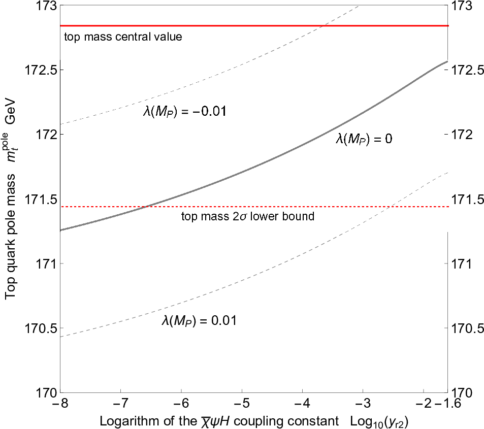
The model has an implication for physics at the Planck scale. The vanishing of the scalar quartic coupling at the Planck scale in a classically scale invariant model, or equivalently, a flat scalar potential at the Planck scale, has been pursued in Ref. [5] in the hope of finding hints for quantum gravity. In previous models, the vanishing of the Higgs quartic coupling is achieved only with the top quark pole mass well below 172 GeV, and hence those models are in tension with top quark mass measurements; note that the ATLAS Collaboration has recently reported the top quark mass to be 172.84±0.70172.84\pm 0.70 GeV [6]. Our model, in contrast, can realize the vanishing of the scalar quartic coupling with the top quark pole mass as large as 172.5 GeV. This is possible owing to contributions of the new fermions to the renormalization group (RG) running of the weak gauge coupling, which enhance this gauge coupling at ultraviolet scales and eventually lift the scalar quartic coupling at the Planck scale through the RG evolution as compared to the SM.

Models where strong dynamics supplies the SM Higgs field mass term in a classically scale invariant setup have been proposed in Ref. [7], which however cannot address the origin of its tachyonic feature. A model similar to ours has been studied in Refs. [8, 9, 10]. Our model is more attractive in that the field content is minimal and thus a more definite prediction for the pNG boson mass spectrum is feasible.

The content of the paper is as follows: In Secion 2, we describe the model and expound how the SM Higgs field mass term is generated from strong dynamics of the S​U​(N)TSU(N)_{T} gauge theory in the classically scale invariant setup. We further evaluate the dynamical scale of the gauge theory based on analogy with QCD. In Section 3, we study phenomenology of the pNG bosons by deriving their mass spectrum and interaction strengths, again relying on analogy with QCD. In Section 4, we demonstrate that the model can achieve the vanishing of the scalar quartic coupling at the Planck scale with the top quark pole mass as large as 172.5 GeV. Section 5 is for the summary and discussions.

2 Model

2.1 Model description and the origin of the Standard Model Higgs field mass

The gauge symmetry of the model is S​U​(N)T×S​U​(3)C×S​U​(2)W×U​(1)YSU(N)_{T}\times SU(3)_{C}\times SU(2)_{W}\times U(1)_{Y}, where S​U​(3)CSU(3)_{C}, S​U​(2)WSU(2)_{W} and U​(1)YU(1)_{Y} are the SM color, weak and hypercharge gauge groups, respectively, and S​U​(N)TSU(N)_{T} is a newly introduced gauge group. We require N≥3N\geq 3. The model includes the same matter fermions as the SM and further contains massless Dirac fermions, χ,ψ\chi,\psi, which are in the fundamental representation of the S​U​(N)TSU(N)_{T} gauge group and are also charged under S​U​(2)W×U​(1)YSU(2)_{W}\times U(1)_{Y} gauge group; χ\chi is an isospin doublet with hypercharge Y=b/2Y=b/2 and ψ\psi is an isospin singlet with hypercharge Y=(b−1)/2Y=(b-1)/2, with bb being an arbitrary number. There also is a massless elementary scalar field, HH, which possesses the same electroweak charge as the SM Higgs field and is a singlet under the S​U​(N)TSU(N)_{T} gauge group. The charges of the fields χ,ψ\chi,\psi and HH are summarized in Table 1.

Field Lorentz S​O​(1,3)SO(1,3) S​U​(N)TSU(N)_{T} S​U​(2)WSU(2)_{W} U​(1)YU(1)_{Y}
HH 1 1 2 1/21/2
χ\chi (2, 2) N 2 b/2b/2
ψ\psi (2, 2) N 1 (b−1)/2(b-1)/2
Table 1: The charges of the fields χ,ψ\chi,\psi and HH. Representations in the Lorentz group, the S​U​(N)TSU(N)_{T} gauge group and the SM electroweak gauge groups S​U​(2)W×U​(1)YSU(2)_{W}\times U(1)_{Y} are displayed. bb is an arbitrary number.

Classical scale invariance forbids Dirac mass terms for χ\chi and ψ\psi and a mass term for HH, while χ\chi and ψ\psi are allowed to have a Yukawa-type coupling with HH. We further assume invariance of the theory under the parity transformation on χ\chi and ψ\psi, χ→γ0​χ\chi\to\gamma_{0}\chi, and ψ→γ0​ψ\psi\to\gamma_{0}\psi. This assumption is required to fully use analogy with QCD. The Lagrangian for χ,ψ\chi,\psi and HH fields thus reads

ℒewsb\displaystyle{\cal L}_{{\rm ewsb}} =|(∂μ+igWWμaτa+i12gYBμ)H|2\displaystyle=\left|\left(\partial_{\mu}+ig_{W}W^{a}_{\mu}\tau^{a}+i\frac{1}{2}g_{Y}B_{\mu}\right)H\right|^{2}
+iχ¯γμ(∂μ+igTXμαTα+igWWμaτa+ib2gYBμ)χ+iψ¯γμ(∂μ+igTXμαTα+ib−12gYBμ)ψ\displaystyle+i\bar{\chi}\gamma^{\mu}\left(\partial_{\mu}+ig_{T}X_{\mu}^{\alpha}T^{\alpha}+ig_{W}W_{\mu}^{a}\tau^{a}+i\frac{b}{2}g_{Y}B_{\mu}\right)\chi+i\bar{\psi}\gamma^{\mu}\left(\partial_{\mu}+ig_{T}X_{\mu}^{\alpha}T^{\alpha}+i\frac{b-1}{2}g_{Y}B_{\mu}\right)\psi
−y​χ¯​ψ​H−y​H†​ψ¯​χ\displaystyle-y\,\bar{\chi}\psi H-y\,H^{\dagger}\bar{\psi}\chi (1)
−λ​(H†​H)2−Yu​q¯​u​ϵ​H∗−Yd​q¯​d​H−Ye​ℓ¯​e​H−H.c.,\displaystyle-\lambda\,(H^{\dagger}H)^{2}-Y_{u}\,\bar{q}u\,\epsilon H^{*}-Y_{d}\,\bar{q}d\,H-Y_{e}\,\bar{\ell}e\,H-{\rm H.c.}, (2)

where yy is a Yukawa coupling constant for HH, χ\chi and ψ\psi fields, which is taken to be real by phase redefinition of ψ\psi field. Here, gTg_{T}, gWg_{W} and gYg_{Y} denote the S​U​(N)TSU(N)_{T}, SM weak and hypercharge gauge coupling constants, XμαX_{\mu}^{\alpha}, WμaW_{\mu}^{a} and BμB_{\mu} denote the corresponding gauge fields, and Tα​(α=1,2,…,N2−1)T^{\alpha}\,(\alpha=1,2,...,N^{2}-1) and τa​(a=1,2,3)\tau^{a}\,(a=1,2,3) are generators of the S​U​(N)TSU(N)_{T} and weak gauge groups, respectively. qq, uu, dd, ℓ\ell and ee respectively denote SM isospin doublet quarks, singlet up-type quarks, down-type quarks, doublet leptons and singlet leptons, YuY_{u}, YdY_{d} and YeY_{e} are coupling constants proportional to the SM Yukawa couplings (flavor indices are omitted), and ϵ\epsilon denotes the antisymmetric tensor in the isospin space.

The S​U​(N)TSU(N)_{T} gauge theory is assumed to become strongly-coupled at infrared scales and induce chiral symmetry breaking and confinement of χ\chi,ψ\psi fields in the same way as QCD. We infer the pattern of chiral symmetry breaking from the most attractive channel hypothesis. When applied to weak and hypercharge gauge boson exchange forces [11], the hypothesis argues that composite operators with the smallest values of the quadratic Casimir operators of S​U​(2)WSU(2)_{W} and U​(1)YU(1)_{Y} groups form condensates, while when applied to the exchange of the elementary scalar HH [12], those with the largest values of the quadratic Casimir operators are expected to form condensates. In the current model, we assume yy to be sufficiently small that the χ¯​ψ​H\bar{\chi}\psi H Yukawa interaction is subdominant compared to the weak and hypercharge gauge interactions, which gives that operators with the smallest quadratic Casimir operators go into chiral condensation, namely, we have

⟨0|χ¯​χ|0⟩\displaystyle\langle 0|\bar{\chi}\chi|0\rangle ≠0,⟨0|χ¯​τa​χ|0⟩=0​(a=1,2,3),⟨0|ψ¯​ψ|0⟩≠0,⟨0|χ¯​ψ|0⟩=0.\displaystyle\neq 0,\ \ \ \ \ \langle 0|\bar{\chi}\tau^{a}\chi|0\rangle=0\ (a=1,2,3),\ \ \ \ \ \langle 0|\bar{\psi}\psi|0\rangle\neq 0,\ \ \ \ \ \langle 0|\bar{\chi}\psi|0\rangle=0. (3)

Note that the electroweak symmetry is maintained at this stage, unlike in the technicolor model [13]. This owes to the fact that χ,ψ\chi,\psi fields are vector-like with respect to the weak and hypercharge gauge groups.

In the mass spectrum below the confinement scale, there exists a scalar meson, Θ\Theta, that corresponds to a scalar bound state of ψ¯​χ\bar{\psi}\chi. We write the mass of Θ\Theta meson as MΘM_{\Theta}, and further define the scalar decay constant for Θ\Theta meson, FΘF_{\Theta}, in the following fashion:

y^​FΘ​MΘ\displaystyle\hat{y}F_{\Theta}M_{\Theta} ≡⟨0|y​ψ¯​χ​(0)|Θ⟩,\displaystyle\equiv\langle 0|y\,\bar{\psi}\chi(0)|\Theta\rangle, (4)

where |Θ⟩|\Theta\rangle denotes the state with one Θ\Theta meson, y​ψ¯​χy\,\bar{\psi}\chi denotes a scalar current accompanied by the coupling constant yy, and y^\hat{y} is a quantity proportional to yy that is RG-invariant in the S​U​(N)TSU(N)_{T} gauge theory. Note that inclusion of the coupling constant yy in the definition of the scalar current is advantageous in that the current becomes independent of the wavefunction renormalization in the S​U​(N)TSU(N)_{T} gauge theory. Below the confinement scale, ψ¯​χ\bar{\psi}\chi term in the Lagrangian Eq. (1) asymptotes to Θ\Theta meson term, and accordingly, y​H​χ¯​ψy\,H\bar{\chi}\psi term becomes a mixing term for HH and Θ\Theta as

y​χ¯​ψ​H\displaystyle y\,\bar{\chi}\psi\,H\ ⇒(y^​FΘ​MΘ)​Θ†​H.\displaystyle\Rightarrow\ (\hat{y}F_{\Theta}M_{\Theta})\,\Theta^{\dagger}H. (5)

The mass matrix for HH and Θ\Theta is thus found to be

−ℒewsb\displaystyle-{\cal L}_{{\rm ewsb}} ⊃(H†Θ†)​(0y^​FΘ​MΘy^​FΘ​MΘMΘ2)​(HΘ).\displaystyle\supset\left(\begin{array}[]{cc}H^{\dagger}&\Theta^{\dagger}\end{array}\right)\left(\begin{array}[]{cc}0&\hat{y}F_{\Theta}M_{\Theta}\\ \hat{y}F_{\Theta}M_{\Theta}&M_{\Theta}^{2}\end{array}\right)\left(\begin{array}[]{c}H\\ \Theta\end{array}\right).

We hereafter concentrate on the limit with small y^\hat{y} that leads to y^​FΘ≪MΘ\hat{y}F_{\Theta}\ll M_{\Theta}. Upon diagonalization, we obtain the following mass terms for mass eigenstate scalar fields H1H_{1} and H2H_{2}:

−ℒewsb\displaystyle-{\cal L}_{{\rm ewsb}} ⊃−(y^​FΘ)2​H1†​H1+MΘ2​H2†​H2,\displaystyle\supset-(\hat{y}F_{\Theta})^{2}\,H_{1}^{\dagger}H_{1}+M_{\Theta}^{2}\,H_{2}^{\dagger}H_{2},
(HΘ)=(cHsH−sHcH)​(H1H2),sH=y^​FΘMΘ,cH=1−12​(y^​FΘ)2MΘ2.\displaystyle\left(\begin{array}[]{c}H\\ \Theta\end{array}\right)=\left(\begin{array}[]{cc}c_{H}&s_{H}\\ -s_{H}&c_{H}\end{array}\right)\left(\begin{array}[]{c}H_{1}\\ H_{2}\end{array}\right),\ \ \ s_{H}=\frac{\hat{y}F_{\Theta}}{M_{\Theta}},\ c_{H}=1-\frac{1}{2}\frac{(\hat{y}F_{\Theta})^{2}}{M_{\Theta}^{2}}.

Since H1H_{1} has a negative mass squared term, it develops a non-zero vacuum expectation value (VEV) and triggers electroweak symmetry breaking. Hence, we identify H1H_{1} with the SM Higgs field. The H1H_{1} field has a quartic coupling and Yukawa couplings induced from Eq. (2) as

−ℒewsb\displaystyle-{\cal L}_{{\rm ewsb}} ⊃λ​cH4​(H1†​H1)2+Yu​cH​q¯​u​ϵ​H1∗+Yd​cH​q¯​d​H1+Ye​cH​ℓ¯​e​H1+H.c.\displaystyle\supset\lambda\,c_{H}^{4}\,(H_{1}^{\dagger}H_{1})^{2}+Y_{u}\,c_{H}\,\bar{q}u\,\epsilon H_{1}^{*}+Y_{d}\,c_{H}\,\bar{q}d\,H_{1}+Y_{e}\,c_{H}\,\bar{\ell}e\,H_{1}+{\rm H.c.}
with​cH=1−12​(y^​FΘ)2MΘ2.\displaystyle{\rm with\ }c_{H}=1-\frac{1}{2}\frac{(\hat{y}F_{\Theta})^{2}}{M_{\Theta}^{2}}. (17)

The mass term, quartic coupling and Yukawa couplings of H1H_{1} field should agree with those of the SM Higgs field at the energy scale of the H2H_{2} mass, that is, MΘM_{\Theta}. These requirements are encapsulated in the following matching conditions:

−12​mh2=(SM​Higgs​field​mass)\displaystyle-\frac{1}{2}m_{h}^{2}=({\rm SM\ Higgs\ field\ mass}) =−(y^​FΘ)2,\displaystyle=-(\hat{y}F_{\Theta})^{2}, (18)
λSM​(MΘ)\displaystyle\lambda^{{\rm SM}}(M_{\Theta}) =λ⁡(MΘ)​cH4=λ⁡(MΘ)​(1−2​(y^​FΘ)2MΘ2),\displaystyle=\lambda(M_{\Theta})\,c_{H}^{4}=\lambda(M_{\Theta})\,\left(1-2\frac{(\hat{y}F_{\Theta})^{2}}{M_{\Theta}^{2}}\right), (19)
YkSM​(MΘ)\displaystyle Y_{k}^{{\rm SM}}(M_{\Theta}) =Yk(MΘ)cH=Yk(MΘ)(1−12(y^​FΘ)2MΘ2)(k=u,d,e),\displaystyle=Y_{k}(M_{\Theta})\,c_{H}=Y_{k}(M_{\Theta})\,\left(1-\frac{1}{2}\frac{(\hat{y}F_{\Theta})^{2}}{M_{\Theta}^{2}}\right)\ \ \ (k=u,d,e),

where mhm_{h} denotes the pole mass of the SM Higgs particle, and λSM​(MΘ)\lambda^{{\rm SM}}(M_{\Theta}) and YuSM​(MΘ)Y_{u}^{{\rm SM}}(M_{\Theta}), YdSM​(MΘ)Y_{d}^{{\rm SM}}(M_{\Theta}), YeSM​(MΘ)Y_{e}^{{\rm SM}}(M_{\Theta}) respectively represent the SM Higgs quartic coupling and SM Yukawa couplings at the energy scale MΘM_{\Theta}.

In this way, the Higgs field mass is generated at the scale determined by the Θ\Theta meson decay constant FΘF_{\Theta} and the χ¯​ψ​H\bar{\chi}\psi H Yukawa coupling constant yy, with the correct negative sign owing to the negative determinant of the mass matrix Eq. (2.1). The scale and sign of the SM Higgs mass term are thus attributed to strong dynamics of the S​U​(N)TSU(N)_{T} gauge theory and its coupling with the elementary scalar field.

We comment in passing that the elementary scalar HH does not have a mixing term with any pNG boson associated with the chiral symmetry breaking, due to the assumption that the theory is invariant under the parity transformation on χ\chi and ψ\psi that makes the Yukawa coupling appear in the form Eq. (1). To prove this, we employ chiral perturbation theory: First we define the fields,

ΨL\displaystyle\Psi_{L} ≡1−γ52​(χψ),ΨR≡1+γ52​(χψ),\displaystyle\equiv\frac{1-\gamma_{5}}{2}\left(\begin{array}[]{c}\chi\\ \psi\end{array}\right),\ \ \ \Psi_{R}\equiv\frac{1+\gamma_{5}}{2}\left(\begin{array}[]{c}\chi\\ \psi\end{array}\right),

in terms of which the Yukawa interaction of Eq. (1) is expressed as 11 1 We here refrain from the phase redefinition of HH that makes yy real.

−ℒ\displaystyle-{\cal L} ⊃Ψ¯L​(0y​Hy∗​H†0)​ΨR+h.c.\displaystyle\supset\bar{\Psi}_{L}\left(\begin{array}[]{cc}0&yH\\ y^{*}H^{\dagger}&0\end{array}\right)\Psi_{R}+{\rm h.c.}

The S​U​(N)TSU(N)_{T} gauge theory possesses approximate U​(3)L×U​(3)RU(3)_{L}\times U(3)_{R} symmetry under the transformation ΨL→UL​ΨL\Psi_{L}\to U_{L}\Psi_{L}, ΨR→UR​ΨR\Psi_{R}\to U_{R}\Psi_{R}, with ULU_{L}, URU_{R} being unitary matrices. Along the chiral symmetry breaking, the axial part U​(3)AU(3)_{A} is spontaneously broken and there appear 9 pNG bosons (one of which gains mass at the dynamical scale from instantons). We parametrize them as

U⁡(x)\displaystyle U(x) =exp⁡( 2​i​Πj​(x)fΠ​λj2+2​i​Π⁡(x)fΠ),\displaystyle=\exp\left(\ 2i\frac{\Pi^{j}(x)}{f_{\Pi}}\frac{\lambda^{j}}{2}+\sqrt{2}i\frac{\Pi(x)}{f_{\Pi}}\ \right), (27)

where Πj​(x)\Pi^{j}(x) (j=1,2,…,8)(j=1,2,...,8) and Π⁡(x)\Pi(x) denote the pNG boson fields, λj\lambda^{j}’s are the Gell-Mann matrices, and fΠf_{\Pi} is the NG boson decay constant. U⁡(x)U(x) transforms under U​(3)L×U​(3)RU(3)_{L}\times U(3)_{R} as

U⁡(x)\displaystyle U(x) →UR​U​(x)​UL†.\displaystyle\to U_{R}U(x)U_{L}^{\dagger}. (28)

Since we can assign to the Yukawa coupling and HH the following spurious transformation property,

(0y​Hy∗​H†0)\displaystyle\left(\begin{array}[]{cc}0&yH\\ y^{*}H^{\dagger}&0\end{array}\right) →UL​(0y​Hy∗​H†0)​UR†,\displaystyle\to U_{L}\left(\begin{array}[]{cc}0&yH\\ y^{*}H^{\dagger}&0\end{array}\right)U_{R}^{\dagger},

the effective Lagrangian reads

ℒe​f​f\displaystyle{\cal L}_{eff} =fΠ24​tr​[(Dμ​U​(x))†​Dμ​U​(x)]−B0​tr​[U⁡(x)​(0y​Hy∗​H†0)]−h.c.,\displaystyle=\frac{f_{\Pi}^{2}}{4}{\rm tr}\left[\left(D_{\mu}U(x)\right)^{\dagger}D^{\mu}U(x)\right]-B_{0}\ {\rm tr}\left[U(x)\left(\begin{array}[]{cc}0&yH\\ y^{*}H^{\dagger}&0\end{array}\right)\right]-{\rm h.c.},

where B0B_{0} is a constant and DμD_{\mu} is a covariant derivative. Based on analogy with QCD, we expect B0B_{0} to be real. Then the second term of Eq. (2.1) is recast into the form,

−ℒe​f​f\displaystyle-{\cal L}_{eff} ⊃B0​tr​[{U⁡(x)+U​(x)†}​(0y​Hy∗​H†0)].\displaystyle\supset B_{0}\ {\rm tr}\left[\ \left\{U(x)+U(x)^{\dagger}\right\}\ \left(\begin{array}[]{cc}0&yH\\ y^{*}H^{\dagger}&0\end{array}\right)\right].

Since the above interaction term is symmetric under the transformation Πj→−Πj\Pi^{j}\to-\Pi^{j} or Π→−Π\Pi\to-\Pi, the couplings between HH and the pNG bosons contain even numbers of pNG bosons and hence no mixing term exists between them.

2.2 Evaluation of the dynamical scale of the S​U​(N)TSU(N)_{T} gauge theory

We evaluate the dynamical scale of the S​U​(N)TSU(N)_{T} gauge theory from the matching condition Eq. (18) under analogy between the S​U​(N)TSU(N)_{T} gauge theory and QCD. This is done by expressing the Θ\Theta meson mass, total width and decay constant in terms of corresponding quantities in QCD, rescaled by the ratio of the dynamical scales of the S​U​(N)TSU(N)_{T} gauge theory and QCD, rr, defined by

r\displaystyle r ≡ΛTΛQ​C​D,\displaystyle\equiv\frac{\Lambda_{T}}{\Lambda_{QCD}}, (37)

where ΛT\Lambda_{T} and ΛQ​C​D\Lambda_{QCD} denote the dynamical scales of the S​U​(N)TSU(N)_{T} gauge theory and QCD, respectively.

Along with rr, a factor depending on N/NcN/N_{c} (Nc=3N_{c}=3 is the number of colors in QCD) appears when one relates some quantities in the S​U​(N)TSU(N)_{T} gauge theory to their QCD counterparts. In this paper, we make the two approximations below:

(α\alpha) The Casimir operator CFC_{F} is approximated as CF=(N2−1)/(2​N)≃N/2C_{F}=(N^{2}-1)/(2N)\simeq N/2.

(β\beta) The contribution of χ,ψ\chi,\psi fermion loop to the gauge field propagator is subdued compared to those of gauge field loop and ghost loop, and is hence negligible. For example, the one-loop correction to the gauge field propagator is proportional to 11​N−2​nf11N-2n_{f} with nfn_{f} being the number of flavors which equals 33 in our model, and this is approximated as 11​N−2​nf=11​N−6≃11​N11N-2n_{f}=11N-6\simeq 11N.

(α\alpha) and (β\beta) give that the coefficient for O⁡(αTn)O(\alpha_{T}^{n}) correction term is proportional to NnN^{n}. It immediately follows that the S​U​(N)TSU(N)_{T} gauge coupling gTg_{T} and the QCD gauge coupling gsg_{s} satisfy gT2​(r​μ)≃(Nc/N)​gs2​(μ)g_{T}^{2}(r\mu)\simeq(N_{c}/N)g_{s}^{2}(\mu). Also, correlation functions of S​U​(N)TSU(N)_{T}-singlet operators, with all operators connected, are obtained by rescaling corresponding correlation functions in QCD by N/NcN/N_{c}, e.g., we have

⟨0|T⁡{f¯​Γ1​f​(x1)​f¯​Γ2​f​(x2)​…​f¯n​Γn​fn​(xn)}|0⟩\displaystyle\langle 0|T\{\bar{f}\Gamma_{1}f(x_{1})\,\bar{f}\Gamma_{2}f(x_{2})\,...\,\bar{f}_{n}\Gamma_{n}f_{n}(x_{n})\}|0\rangle =NNc​r3​n​⟨0|T⁡{q¯​Γ1​q​(x1)​q¯​Γ2​q​(x2)​…​q¯​Γn​q​(xn)}|0⟩,\displaystyle=\frac{N}{N_{c}}r^{3n}\,\langle 0|T\{\bar{q}\Gamma_{1}q(x_{1})\,\bar{q}\Gamma_{2}q(x_{2})\,...\,\bar{q}\Gamma_{n}q(x_{n})\}|0\rangle, (38)

where f¯​Γi​f\bar{f}\Gamma_{i}f and q¯​Γi​q\bar{q}\Gamma_{i}q (i=1,2,…,ni=1,2,...,n) represent S​U​(N)TSU(N)_{T}-singlet and QCD-singlet bilinear operators of massless Dirac fermions in the fundamental representation of the S​U​(N)TSU(N)_{T} and QCD gauge groups, respectively, with Γi\Gamma_{i} being a combination of the gamma matrices. As a corollary, the wavefunction overlap of a one-meson-state with a S​U​(N)TSU(N)_{T}-singlet current operator roughly scales by N/Nc\sqrt{N/N_{c}}, because the two-point self-correlation function of that current operator scales by N/NcN/N_{c}. In particular, the decay constant for a Nambu-Goldstone (NG) boson is proportional to N/Nc\sqrt{N/N_{c}}. Moreover, the decay amplitude for a meson decaying into two mesons through the S​U​(N)TSU(N)_{T} gauge interaction scales by (N/Nc)−1/2(N/N_{c})^{-1/2}. This is because a correlation function for three S​U​(N)TSU(N)_{T}-singlet current operators scales by N/NcN/N_{c}, and when the current operators asymptote to one-meson creation operators, a factor (N/Nc)−1/2(N/N_{c})^{-1/2} appears for each current, which leads to an overall factor of (N/Nc){(N/Nc)−1/2}3=(N/Nc)−1/2(N/N_{c})\{(N/N_{c})^{-1/2}\}^{3}=(N/N_{c})^{-1/2} for the decay amplitude.

2.2.1 Θ\Theta meson mass MΘM_{\Theta}

We evaluate the Θ\Theta meson mass MΘM_{\Theta} by regarding the K0∗​(1430)K_{0}^{*}(1430) meson as a QCD analog of the Θ\Theta meson for two reasons 22 2 For studies on scalar mesons, see Ref. [15] and references therein. :

(i)It is likely that K0∗​(1430)K_{0}^{*}(1430) belongs to a nonet of quark-anti-quark bound states whereas K0∗​(800)K_{0}^{*}(800) belongs a nonet of diquark-anti-diquark bound states, notably because the K0∗​(800)K_{0}^{*}(800) mass is considerably smaller than the a0​(980)a_{0}(980) mass, which suggests that K0∗​(800)K_{0}^{*}(800) is mainly a bound state of (s,q,q¯,q¯′)(s,q,\bar{q},\bar{q}^{\prime}) and a0​(980)a_{0}(980) is that of (s,q,s¯,q¯′)(s,q,\bar{s},\bar{q}^{\prime}) (q,q′q,q^{\prime} denote up and down quarks and ss denotes strange quark). Hence, K0∗​(1430)K_{0}^{*}(1430) meson corresponds to the lightest χ¯​ψ\bar{\chi}\psi scalar bound state, i.e., Θ\Theta meson.

(ii)K0∗​(1430)K_{0}^{*}(1430) meson and Θ\Theta meson do not mix with glueball state and its S​U​(N)TSU(N)_{T}-gauge-theory counterpart due to non-zero strangeness and electroweak charge, respectively.

Analogy between Θ\Theta meson and K0∗​(1430)K_{0}^{*}(1430) meson enables us to express the Θ\Theta meson mass MΘM_{\Theta} in terms of the K0∗​(1430)K_{0}^{*}(1430) mass, mK0∗​(1430)m_{K_{0}^{*}(1430)}, as

MΘ\displaystyle M_{\Theta} =r​mK0∗​(1430).\displaystyle=r\,m_{K_{0}^{*}(1430)}. (39)

The experimental central value [14] gives MΘ=r⋅1.425M_{\Theta}=r\cdot 1.425 GeV.

2.2.2 Θ\Theta meson total width ΓΘ\Gamma_{\Theta}

The Θ\Theta meson total width, ΓΘ\Gamma_{\Theta}, can be written with the K0∗​(1430)K_{0}^{*}(1430) meson total width, ΓK0∗​(1430)\Gamma_{K_{0}^{*}(1430)}. In doing so, we remind that about 90% of K0∗​(1430)K_{0}^{*}(1430) decays as K0∗​(1430)→K​πK_{0}^{*}(1430)\to K\pi [14], in which process the K,πK,\pi meson masses modify the phase space, while the corresponding pNG bosons in the S​U​(N)TSU(N)_{T} gauge theory are nearly massless due to zero current mass. Hence, we rescale the K0∗​(1430)K_{0}^{*}(1430) total width by the phase space ratio, together with the dynamical scale ratio rr and the factor (N/Nc)−1(N/N_{c})^{-1}, to evaluate ΓΘ\Gamma_{\Theta}. It is thus found to be

ΓΘ\displaystyle\Gamma_{\Theta} =r​NcN​11−2​mπ2+mK2mK0∗​(1430)2+(mπ2−mK2)2mK0∗​(1430)4​ΓK0∗​(1430),\displaystyle=r\,\frac{N_{c}}{N}\,\frac{1}{\sqrt{1-2\frac{m_{\pi}^{2}+m_{K}^{2}}{m_{K_{0}^{*}(1430)}^{2}}+\frac{(m_{\pi}^{2}-m_{K}^{2})^{2}}{m_{K_{0}^{*}(1430)}^{4}}}}\,\Gamma_{K_{0}^{*}(1430)}, (40)

where mπm_{\pi} and mKm_{K} denote the π\pi and KK masses, respectively. The experimental central values [14] give ΓΘ=r⁡(Nc/N)⋅0.311\Gamma_{\Theta}=r(N_{c}/N)\cdot 0.311 GeV.

2.2.3 Θ\Theta meson scalar decay constant FΘF_{\Theta}

Since a QCD analog of the Θ\Theta meson scalar decay constant FΘ=⟨0|y​ψ¯​χ|Θ⟩/(y^​MΘ)F_{\Theta}=\langle 0|y\,\bar{\psi}\chi|\Theta\rangle/(\hat{y}M_{\Theta}) has not been measured, we evaluate it by the aid of explicit calculations. To this end, we confront the spectral density of states that couple to the scalar current y​χ¯​ψy\,\bar{\chi}\psi, with the two-point self-correlation function of that scalar current for large space-like momenta; the former spectral density contains the term y^​FΘ​MΘ\hat{y}F_{\Theta}M_{\Theta}, as it quantifies the coupling of the one-Θ\Theta-meson state with the scalar current. The latter correlation function can be described with perturbative calculation in the S​U​(N)TSU(N)_{T} gauge theory and with empirical vacuum condensates. To embody the idea, we formulate the correlation function, Πy​χ¯​ψ​(q2)\Pi_{y\bar{\chi}\psi}(q^{2}), and the spectral density, ρs​(s)\rho_{s}(s), in the following fashion 33 3 We insert the factor 1/21/2 in Eq. (41) to cancel the S​U​(2)WSU(2)_{W} degree of freedom of χ\chi. :

Πy​χ¯​ψ​(q2)\displaystyle\Pi_{y\bar{\chi}\psi}(q^{2}) ≡12​i​∫d4​x​ei​q​x​⟨0|T⁡{y​χ¯​(x)​ψ​(x)​y​ψ¯​(0)​χ​(0)}|0⟩,\displaystyle\equiv\frac{1}{2}i\int{\rm d}^{4}x\,e^{iqx}\langle 0|T\left\{y\,\bar{\chi}(x)\psi(x)\ y\,\bar{\psi}(0)\chi(0)\right\}|0\rangle, (41)
ρs​(s)\displaystyle\rho_{s}(s) ≡Im​Πy​χ¯​ψ​(s)for​s≥0.\displaystyle\equiv{\rm Im}\Pi_{y\bar{\chi}\psi}(s)\ \ \ \ \ {\rm for}\ s\geq 0. (42)

We relate the spectral density to the correlation function for space-like momenta using the Cauchy’s theorem. Since no one-massless-particle state couples to the scalar current, we have

lim|q2|→0q2​Πy​χ¯​ψ​(q2)\displaystyle\lim_{|q^{2}|\to 0}\,q^{2}\Pi_{y\bar{\chi}\psi}(q^{2}) =0\displaystyle=0 (43)

for complex q2q^{2}, which allows us to use the Cauchy’s theorem to obtain

∫0s0ds{P(s)−P(s0)}1πImΠy​χ¯​ψ(s)=−12​π​i∮|q2|=s0dq2{P(q2)−P(s0)}Πy​χ¯​ψ(q2),\displaystyle\int_{0}^{s_{0}}{\rm d}s\,\{P(s)-P(s_{0})\}\,\frac{1}{\pi}{\rm Im}\Pi_{y\bar{\chi}\psi}(s)=-\frac{1}{2\pi i}\oint_{|q^{2}|=s_{0}}{\rm d}q^{2}\,\{P(q^{2})-P(s_{0})\}\,\Pi_{y\bar{\chi}\psi}(q^{2}), (44)

where s0s_{0} can take any real positive value and P⁡(s)P(s) can be any analytic function. Here, on the right-hand side, the correlation function for complex q2q^{2} off the real positive axis can be derived through analytic continuation from space-like momenta, while the discontinuity of the correlation function at q2=s0q^{2}=s_{0} is avoided as the function P⁡(q2)−P⁡(s0)P(q^{2})-P(s_{0}) vanishes there. The left-hand side includes y^​FΘ​MΘ\hat{y}F_{\Theta}M_{\Theta}, and the right-hand side is calculable by perturbation theory and operator product expansion in the S​U​(N)TSU(N)_{T} gauge theory if s0s_{0} is taken sufficiently large that these calculations are valid. Therefore, the equality Eq. (44) enables us to evaluate y^​FΘ​MΘ\hat{y}F_{\Theta}M_{\Theta} through analytic calculations. The use of Eq. (44) for such s0s_{0} constitutes the basis for the finite energy sum rules [16].

First we express the spectral density ρs​(s)\rho_{s}(s) in terms of y^​FΘ​MΘ\hat{y}F_{\Theta}M_{\Theta} based on the following two assumptions on quantum states that couple to the scalar current y​χ¯​ψy\,\bar{\chi}\psi:

(i) In the range MΘ2−r2⋅1​GeV2≲s≲MΘ2+r2⋅1​GeV2M_{\Theta}^{2}-r^{2}\cdot 1~{\rm GeV}^{2}\lesssim s\lesssim M_{\Theta}^{2}+r^{2}\cdot 1~{\rm GeV}^{2}, the spectral density ρs​(s)\rho_{s}(s) is dominated by contributions from the Θ\Theta meson resonance.

(ii) The Θ\Theta meson resonance is well approximated by the relativistic Breit-Wigner function.

These ansaetze find no support from hadron physics experiments, even given analogy between Θ\Theta meson and K0∗​(1430)K_{0}^{*}(1430) meson, because an elementary scalar current that couples to light quarks has not been measured. Nevertheless, SS-wave K​πK\pi scattering data from the LASS experiment [17] hint us that the K0∗​(1430)K_{0}^{*}(1430) meson resonance may dominantly couple to d¯​s\bar{d}s scalar current (dd and ss respectively denote down and strange quarks) for invariant mass mK0∗​(1430)2−1​GeV2≲s≲mK0∗​(1430)2+1​GeV2m_{K_{0}^{*}(1430)}^{2}-1~{\rm GeV}^{2}\lesssim s\lesssim m_{K_{0}^{*}(1430)}^{2}+1~{\rm GeV}^{2}, which is rendered into the assumption (i) through the rescaling. The same data also suggest that the K0∗​(1430)K_{0}^{*}(1430) meson resonance can be fit with the relativistic Breit-Wigner function. Once one accepts (i) and (ii), the spectral density satisfies

for\displaystyle{\rm for}\ MΘ2−r2⋅1​GeV2≲s≲MΘ2+r2⋅1​GeV2,\displaystyle M_{\Theta}^{2}-r^{2}\cdot 1~{\rm GeV}^{2}\lesssim s\lesssim M_{\Theta}^{2}+r^{2}\cdot 1~{\rm GeV}^{2},
ρs​(s)\displaystyle\rho_{s}(s) =1π​Im​Πy​χ¯​ψ​(s)\displaystyle=\frac{1}{\pi}{\rm Im}\Pi_{y\bar{\chi}\psi}(s)
=1π​Im​[⟨0|y​ψ¯​χ|Θ⟩​1s−MΘ2+i​MΘ​ΓΘ​⟨Θ|y​χ¯​ψ|0⟩]\displaystyle=\frac{1}{\pi}{\rm Im}\left[\,\langle 0|y\,\bar{\psi}\chi|\Theta\rangle\frac{1}{s-M_{\Theta}^{2}+iM_{\Theta}\Gamma_{\Theta}}\langle\Theta|y\,\bar{\chi}\psi|0\rangle\,\right]
=(y^​FΘ​MΘ)2​1π​MΘ​ΓΘ(s−MΘ2)2+MΘ2​ΓΘ2.\displaystyle=(\hat{y}F_{\Theta}M_{\Theta})^{2}\,\frac{1}{\pi}\frac{M_{\Theta}\Gamma_{\Theta}}{(s-M_{\Theta}^{2})^{2}+M_{\Theta}^{2}\Gamma_{\Theta}^{2}}. (45)

Note here that since Θ\Theta meson decays into two pNG bosons, which are nearly massless due to the absence of current mass, the Breit-Wigner function reduces to the form as appears in Eq. (45).

Next we present the scalar current correlation function for space-like momenta q2<0q^{2}<0 as a perturbative series of the S​U​(N)TSU(N)_{T} gauge coupling and an operator product expansion involving vacuum condensates, following analogous calculations for QCD in Refs. [18, 19, 20, 21]. The scalar current correlation function is given, for q2<0q^{2}<0, by

Πy​χ¯​ψ​(q2)=A​q2+y2​(μ2)​N8​π2​(−q2)​log⁡(−q2μ2)​{ 1+∑k=1∞(αT​(μ2)π)k​∑l=0kdk,l​(CF,CA)​logl⁡(−q2μ2)}\displaystyle\Pi_{y\bar{\chi}\psi}(q^{2})=A\,q^{2}+y^{2}(\mu^{2})\frac{N}{8\pi^{2}}(-q^{2})\log\left(\frac{-q^{2}}{\mu^{2}}\right)\left\{\,1+\sum_{k=1}^{\infty}\,\left(\frac{\alpha_{T}(\mu^{2})}{\pi}\right)^{k}\,\sum_{l=0}^{k}\,d_{k,l}(C_{F},C_{A})\,\log^{l}\left(\frac{-q^{2}}{\mu^{2}}\right)\,\right\}
+18​π​1(−q2)​y2​(μ2)​⟨0|αT​Xμ​να​Xα​μ​ν|0⟩\displaystyle+\frac{1}{8\pi}\frac{1}{(-q^{2})}\,y^{2}(\mu^{2})\,\langle 0|\alpha_{T}X_{\mu\nu}^{\alpha}X^{\alpha\mu\nu}|0\rangle
+2​π​1(−q2)2​y2​(μ2)​⟨0|αT​{χ¯​σμ​ν​Tα​ψ​ψ¯​σμ​ν​Tα​χ+13​(χ¯​γμ​Tα​χ+2​ψ¯​γμ​Tα​ψ)​(χ¯​γμ​Tα​χ+ψ¯​γμ​Tα​ψ)}|0⟩\displaystyle+2\pi\frac{1}{(-q^{2})^{2}}y^{2}(\mu^{2})\langle 0|\alpha_{T}\{\,\bar{\chi}\sigma_{\mu\nu}T^{\alpha}\psi\,\bar{\psi}\sigma^{\mu\nu}T^{\alpha}\chi+\frac{1}{3}(\bar{\chi}\gamma_{\mu}T^{\alpha}\chi+2\bar{\psi}\gamma_{\mu}T^{\alpha}\psi)(\bar{\chi}\gamma^{\mu}T^{\alpha}\chi+\bar{\psi}\gamma^{\mu}T^{\alpha}\psi)\,\}|0\rangle
+(other​vacuum​condensates)+(O⁡(αT​(μ2)/π)​corrections​to​vacuum​condensates).\displaystyle+({\rm other\ vacuum\ condensates})+(\ O(\alpha_{T}(\mu^{2})/\pi){\rm\ corrections\ to\ vacuum\ condensates}\ ). (46)

Here, AA is a constant of no interest, αT≡gT2/(4​π)\alpha_{T}\equiv g_{T}^{2}/(4\pi), CF=(N2−1)/(2​N)C_{F}=(N^{2}-1)/(2N), CA=NC_{A}=N, TαT^{\alpha} denotes S​U​(N)TSU(N)_{T} group generators, and Xμ​ναX_{\mu\nu}^{\alpha} denotes the S​U​(N)TSU(N)_{T} gauge field strength. μ\mu denotes the renormalization scale in the M​S¯\overline{MS} scheme for the correlation function itself, the running coupling constant y⁡(μ2)y(\mu^{2}) and the running gauge coupling constant αT​(μ2)\alpha_{T}(\mu^{2}), which is taken to be common for simplicity. dk,l​(CF,CA)d_{k,l}(C_{F},C_{A})’s are coefficients that depend on CF,CAC_{F},C_{A}, whose explicit forms are found in Ref. [18]. The first term in the last line represents vacuum condensates of other operators, which are known to be subdominant compared to the field strength condensate and four-fermion condensate for −q2≳r2⋅1-q^{2}\gtrsim r^{2}\cdot 1 GeV2. We stress that fermion bilinear condensates ⟨0|f¯​f|0⟩\langle 0|\bar{f}f|0\rangle (f=χ,ψf=\chi,\psi) do not enter into Eq. (46) due to the absence of χ,ψ\chi,\psi current mass.

Finally, we associate the spectral density Eq. (45) with the correlation function Eq. (46) through the Cauchy’s theorem Eq. (44). For an arbitrary analytic function P⁡(s)P(s), we choose

P⁡(s)\displaystyle P(s) =exp[−(s−MΘ2)2Δ​s2]withΔs=r2⋅1GeV2,\displaystyle=\exp\left[\,-\frac{(s-M_{\Theta}^{2})^{2}}{\Delta s^{2}}\,\right]\ \ {\rm with\ \ }\Delta s=r^{2}\cdot 1~{\rm GeV}^{2}, (47)

whose shape is depicted in Figure 1.

Refer to caption
Figure 1: The function P⁡(s)P(s) Eq. (47) in the range 0≤s≤r2⋅4​GeV20\leq s\leq r^{2}\cdot 4~{\rm GeV}^{2}. The solid vertical line corresponds to s=MΘ2s=M_{\Theta}^{2} and dashed lines to s=MΘ2±r2⋅1​GeV2s=M_{\Theta}^{2}\pm r^{2}\cdot 1~{\rm GeV}^{2}.

The function P⁡(s)P(s) as given in Eq. (47) is beneficial for extracting the Θ\Theta meson contribution to the spectral density, because P⁡(s)P(s) is sizable only in the range MΘ2−r2⋅1​GeV2≲s≲MΘ2+r2⋅1​GeV2M_{\Theta}^{2}-r^{2}\cdot 1~{\rm GeV}^{2}\lesssim s\lesssim M_{\Theta}^{2}+r^{2}\cdot 1~{\rm GeV}^{2}, where the Θ\Theta meson resonance is assumed to dominate the spectral density, while contributions from the spectral density outside the range are exponentially suppressed. We set the common renormalization scale for Πy​χ¯​ψ​(q2)\Pi_{y\bar{\chi}\psi}(q^{2}) as μ2=s0\mu^{2}=s_{0}. We thus obtain

∫0s0ds{P(s)−P(s0)}ρs(s)=−12​π​i∮|q2|=s0dq2{P(q2)−P(s0)}Πy​χ¯​ψ(q2)\displaystyle\int_{0}^{s_{0}}{\rm d}s\,\{P(s)-P(s_{0})\}\,\rho_{s}(s)=-\frac{1}{2\pi i}\oint_{|q^{2}|=s_{0}}{\rm d}q^{2}\,\{P(q^{2})-P(s_{0})\}\,\Pi_{y\bar{\chi}\psi}(q^{2})
⟺\displaystyle\Longleftrightarrow
(y^​FΘ​MΘ)2​∫0s0d​s​{P⁡(s)−P⁡(s0)}​1π​MΘ​ΓΘ(s−MΘ2)2+MΘ2​ΓΘ2\displaystyle(\hat{y}F_{\Theta}M_{\Theta})^{2}\,\int_{0}^{s_{0}}{\rm d}s\,\{P(s)-P(s_{0})\}\,\frac{1}{\pi}\frac{M_{\Theta}\Gamma_{\Theta}}{(s-M_{\Theta}^{2})^{2}+M_{\Theta}^{2}\Gamma_{\Theta}^{2}}
=y2​(s0)​N8​π2​s02​{B0+∑k=1∞(αT​(s0)π)k​∑l=0kdk,l​(CF,CA)​Bl+1}\displaystyle=y^{2}(s_{0})\frac{N}{8\pi^{2}}\,s_{0}^{2}\,\left\{\,B_{0}+\sum_{k=1}^{\infty}\,\left(\frac{\alpha_{T}(s_{0})}{\pi}\right)^{k}\,\sum_{l=0}^{k}\,d_{k,l}(C_{F},C_{A})\,B_{l+1}\,\right\}
+18​π​y2​(s0)​C1​⟨0|αT​Xμ​να​Xα​μ​ν|0⟩\displaystyle+\frac{1}{8\pi}\,y^{2}(s_{0})\,C_{1}\,\langle 0|\alpha_{T}X_{\mu\nu}^{\alpha}X^{\alpha\mu\nu}|0\rangle
+2​π​y2​(s0)​C2​1s0​⟨0|αT​{χ¯​σμ​ν​Tα​ψ​ψ¯​σμ​ν​Tα​χ+13​(χ¯​γμ​Tα​χ+2​ψ¯​γμ​Tα​ψ)​(χ¯​γμ​Tα​χ+ψ¯​γμ​Tα​ψ)}|0⟩\displaystyle+2\pi y^{2}(s_{0})\,C_{2}\,\frac{1}{s_{0}}\langle 0|\alpha_{T}\{\,\bar{\chi}\sigma_{\mu\nu}T^{\alpha}\psi\,\bar{\psi}\sigma^{\mu\nu}T^{\alpha}\chi+\frac{1}{3}(\bar{\chi}\gamma_{\mu}T^{\alpha}\chi+2\bar{\psi}\gamma_{\mu}T^{\alpha}\psi)(\bar{\chi}\gamma^{\mu}T^{\alpha}\chi+\bar{\psi}\gamma^{\mu}T^{\alpha}\psi)\,\}|0\rangle
+(other​vacuum​condensates)+(O⁡(αT​(s0)/π)​corrections​to​vacuum​condensates),\displaystyle+({\rm other\ vacuum\ condensates})+(\ O(\alpha_{T}(s_{0})/\pi){\rm\ corrections\ to\ vacuum\ condensates}\ ), (48)

where BlB_{l}’s and ClC_{l}’s are numbers defined as

Bl\displaystyle B_{l} ≡−1s0212​π​i∮|q2|=s0dq2{P(q2)−P(s0)}(−q2)logl+1(−q2s0)\displaystyle\equiv-\frac{1}{s_{0}^{2}}\,\frac{1}{2\pi i}\oint_{|q^{2}|=s_{0}}{\rm d}q^{2}\,\{P(q^{2})-P(s_{0})\}\,(-q^{2})\log^{l+1}\left(\frac{-q^{2}}{s_{0}}\right)
=12​π​i​∫02​πd​θ​i​e2​i​θ​{exp⁡[−(s0​ei​θ−MΘ2)22​M4]−exp⁡[−(s0−MΘ2)22​M4]}​{i⁡(θ−π)}l+1,\displaystyle=\frac{1}{2\pi i}\int_{0}^{2\pi}{\rm d}\theta\,i\,e^{2i\theta}\,\left\{\,\exp\left[\,-\frac{(s_{0}e^{i\theta}-M_{\Theta}^{2})^{2}}{2M^{4}}\,\right]-\exp\left[\,-\frac{(s_{0}-M_{\Theta}^{2})^{2}}{2M^{4}}\,\right]\,\right\}\,\{i(\theta-\pi)\}^{l+1},
Cl\displaystyle C_{l} ≡−s0l−112​π​i∮|q2|=s0dq2{P(q2)−P(s0)}1(−q2)l\displaystyle\equiv-s_{0}^{l-1}\,\frac{1}{2\pi i}\oint_{|q^{2}|=s_{0}}{\rm d}q^{2}\,\{P(q^{2})-P(s_{0})\}\,\frac{1}{(-q^{2})^{l}}
=(−1)l+12​π​i​∫02​πd​θ​i​e−i​θ​(l−1)​{exp⁡[−(s0​ei​θ−MΘ2)22​M4]−exp⁡[−(s0−MΘ2)22​M4]}.\displaystyle=\frac{(-1)^{l+1}}{2\pi i}\int_{0}^{2\pi}{\rm d}\theta\,i\,e^{-i\theta(l-1)}\,\left\{\,\exp\left[\,-\frac{(s_{0}e^{i\theta}-M_{\Theta}^{2})^{2}}{2M^{4}}\,\right]-\exp\left[\,-\frac{(s_{0}-M_{\Theta}^{2})^{2}}{2M^{4}}\,\right]\,\right\}. (49)

One can derive (y^​FΘ​MΘ)2(\hat{y}F_{\Theta}M_{\Theta})^{2} from the equality Eq. (48). The derived value would not depend on s0s_{0} if the true spectral density were used and the correlation function were calculated to all orders in perturbation theory and in operator product expansion. In reality, it does exhibit a s0s_{0} dependence due to the error of spectral density assumed and the truncation of perturbative series and operator product expansion. Nevertheless, we argue that a value of (y^​FΘ​MΘ)2(\hat{y}F_{\Theta}M_{\Theta})^{2} that is most stable against variations of s0s_{0} is a physically meaningful estimate for (y^​FΘ​MΘ)2(\hat{y}F_{\Theta}M_{\Theta})^{2}. To search for such a value, we numerically evaluate both sides of Eq. (48) to express (y^​FΘ​MΘ)2(\hat{y}F_{\Theta}M_{\Theta})^{2} as a function of s0s_{0}

For the left-hand side of Eq. (48), we numerically integrate the relativistic Breit-Wigner function Eq. (45) multiplied by the function P⁡(s)−P⁡(s0)P(s)-P(s_{0}) Eq. (47), substituting the previously evaluated values of Θ\Theta meson mass MΘM_{\Theta} and total width ΓΘ\Gamma_{\Theta}. Contributions from states other than the Θ\Theta meson resonance are ignored, as they are exponentially suppressed by the function P⁡(s)P(s).

In the right-hand side of Eq. (48), we evaluate the perturbative series to the order of αT4\alpha_{T}^{4}. We quote the analytic expressions of d1,ld_{1,l}, d2,ld_{2,l} and d3,ld_{3,l} from Ref. [18]. As for d4,0d_{4,0}, only the formula for N=3N=3 is available in the literature. Therefore, we estimate d4,0d_{4,0} for general NN by rescaling the analytic expression of d4,0d_{4,0} for N=3N=3 in Ref. [19] by the following rule, based on the approximation with CF=(N2−1)/(2​N)≃N/2C_{F}=(N^{2}-1)/(2N)\simeq N/2; the nf0n_{f}^{0} term is rescaled by (N/3)4(N/3)^{4}; the nf1n_{f}^{1} term is rescaled by (N/3)3(N/3)^{3}; the nf2n_{f}^{2} term is rescaled by (N/3)2(N/3)^{2}; the nf3n_{f}^{3} term is rescaled by N/3N/3, with nfn_{f} denoting the number of quark flavors. d4,1,d4,2,d4,3,d4,4d_{4,1},d_{4,2},d_{4,3},d_{4,4} are calculated from terms of order αT3\alpha_{T}^{3} or below through RG equations. We separately evaluate αT​(s0)\alpha_{T}(s_{0}) and y⁡(s0)y(s_{0}) by solving RG equations; to obtain αT​(s0)\alpha_{T}(s_{0}), we employ the O⁡(αs4)O(\alpha_{s}^{4}) RG equation for the QCD gauge coupling with the replacement of CF,CAC_{F},C_{A} with those for the S​U​(N)TSU(N)_{T} gauge group, and impose an initial condition at the scale μ=r⋅1.777\mu=r\cdot 1.777 GeV. The equations are given below:

d​αT​(μ2)d​log⁡μ2\displaystyle\frac{{\rm d}\alpha_{T}(\mu^{2})}{{\rm d}\log\mu^{2}} =−β1​(CF)​αT2​(μ2)−β2​(CF,CA)​αT3​(μ2)−β3​(CF,CA)​αT4​(μ2),\displaystyle=-\beta_{1}(C_{F})\,\alpha_{T}^{2}(\mu^{2})-\beta_{2}(C_{F},C_{A})\,\alpha_{T}^{3}(\mu^{2})-\beta_{3}(C_{F},C_{A})\,\alpha_{T}^{4}(\mu^{2}),
αT​(μ2)\displaystyle\alpha_{T}(\mu^{2}) =NcN⋅0.33atμ=r⋅1.777GeV,\displaystyle=\frac{N_{c}}{N}\cdot 0.33\ \ {\rm at}\ \ \mu=r\cdot 1.777~{\rm GeV}, (50)

where the forms of β1,β2,β3\beta_{1},\beta_{2},\beta_{3} are found in Ref. [24]. Here, the initial condition is based on the QCD gauge coupling constant at the τ\tau lepton mass scale mτ=1.777m_{\tau}=1.777 GeV studied in Ref. [25], which is rescaled by the factor Nc/NN_{c}/N under the approximations (α),(β)(\alpha),(\beta) in Section 2.2. To gain y⁡(s0)y(s_{0}), we exploit the O⁡(αs4)O(\alpha_{s}^{4}) RG equation for the running current quark mass in Ref. [23] by exchanging CF,CAC_{F},C_{A} with those for the S​U​(N)TSU(N)_{T} gauge group. This is justifiable because the coupling constant yy and the current quark mass obey the same RG equation in the S​U​(N)TSU(N)_{T} gauge theory and QCD. Since the overall scale of the coupling constant yy is a free parameter of the model, we express y⁡(s0)y(s_{0}) as normalized by the value at one particular scale. For later convenience, we express y⁡(s0)y(s_{0}) in terms of yy evaluated at μ=r⋅2\mu=r\cdot 2 GeV scale in the M​S¯\overline{MS} scheme, which we denote by yr​2≡y⁡(μ2=r2⋅22​GeV2)y_{r2}\equiv y(\mu^{2}=r^{2}\cdot 2^{2}~{\rm GeV}^{2}).

The vacuum condensates are assessed by analogy with QCD; using the values of QCD gluon condensate and four-quark condensate obtained from e+​e−e^{+}e^{-} collisions, heavy quarkonia and τ\tau lepton decays in Ref. [22], we evaluate them as

18​π​⟨0|αT​Xμ​να​Xα​μ​ν|0⟩≃18​π​NNc​r4​⟨0|αs​Gμ​νa​Ga​μ​ν|0⟩=18​π​NNc​r4⋅6.8×10−2​GeV4,\displaystyle\frac{1}{8\pi}\langle 0|\alpha_{T}X_{\mu\nu}^{\alpha}X^{\alpha\mu\nu}|0\rangle\simeq\frac{1}{8\pi}\,\frac{N}{N_{c}}\,r^{4}\,\langle 0|\alpha_{s}G_{\mu\nu}^{a}G^{a\mu\nu}|0\rangle=\frac{1}{8\pi}\,\frac{N}{N_{c}}\,r^{4}\cdot 6.8\times 10^{-2}\,{\rm GeV}^{4}, (51)
2​π​⟨0|αT​{χ¯​σμ​ν​Tα​ψ​ψ¯​σμ​ν​Tα​χ+13​(χ¯​γμ​Tα​χ+2​ψ¯​γμ​Tα​ψ)​(χ¯​γμ​Tα​χ+ψ¯​γμ​Tα​ψ)}|0⟩\displaystyle 2\pi\langle 0|\alpha_{T}\{\,\bar{\chi}\sigma_{\mu\nu}T^{\alpha}\psi\,\bar{\psi}\sigma^{\mu\nu}T^{\alpha}\chi+\frac{1}{3}(\bar{\chi}\gamma_{\mu}T^{\alpha}\chi+2\bar{\psi}\gamma_{\mu}T^{\alpha}\psi)(\bar{\chi}\gamma^{\mu}T^{\alpha}\chi+\bar{\psi}\gamma^{\mu}T^{\alpha}\psi)\,\}|0\rangle
≃−22​π3​N2−1N2​ρ​αT​(⟨0|f¯​f|0⟩)2≃−22​π3​N2−1N2​NNc​r6​ρ​αs​(⟨0|q¯​q|0⟩)2\displaystyle\simeq-\frac{22\pi}{3}\frac{N^{2}-1}{N^{2}}\,\rho\alpha_{T}(\langle 0|\bar{f}f|0\rangle)^{2}\simeq-\frac{22\pi}{3}\frac{N^{2}-1}{N^{2}}\frac{N}{N_{c}}\,r^{6}\,\rho\alpha_{s}(\langle 0|\bar{q}q|0\rangle)^{2}
=−22​π3N2−1N2NNcr6⋅4.5×10−4GeV6,\displaystyle=-\frac{22\pi}{3}\frac{N^{2}-1}{N^{2}}\frac{N}{N_{c}}\,r^{6}\cdot 4.5\times 10^{-4}\,{\rm GeV}^{6}, (52)

where in Eq. (52), ff represents one massless Dirac fermion in the fundamental representation of the S​U​(N)TSU(N)_{T} gauge group, and ρ\rho denotes the ratio of four-quark condensate and the square of quark bilinear condensate. The factor N/NcN/N_{c} ensues from the rescaling of the correlation functions of operators in the adjoint representation, which scale by N2/Nc2N^{2}/N_{c}^{2}, and that of the gauge coupling, which scales by Nc/NN_{c}/N.

As a reference, we numerically express the perturbative series and the two vacuum condensates for N=3,6N=3,6 and for s0=r2⋅32​GeV2,r2⋅52​GeV2s_{0}=r^{2}\cdot 3^{2}~{\rm GeV}^{2},\,r^{2}\cdot 5^{2}~{\rm GeV}^{2}. Also shown is the value of the gauge coupling a≡(N/3)​αT​(s0)/πa\equiv(N/3)\alpha_{T}(s_{0})/\pi for each s0s_{0} and NN. We comment that for s0<r2⋅32​GeV2s_{0}<r^{2}\cdot 3^{2}~{\rm GeV}^{2}, the perturbative series does not show good convergence, while for s0>r2⋅52​GeV2s_{0}>r^{2}\cdot 5^{2}~{\rm GeV}^{2}, numerical calculation of the contour integral is computationally expensive due to a rapid oscillation of the function P⁡(q2)P(q^{2}) for complex q2q^{2}.

For​N=3​and​s0=r2⋅32​GeV2,\displaystyle{\rm For\ }N=3{\rm\ and\ }s_{0}=r^{2}\cdot 3^{2}~{\rm GeV}^{2},
−12​π​i∮|q2|=s0dq2{P(q2)−P(s0)}Πy​χ¯​ψ(q2)\displaystyle-\frac{1}{2\pi i}\oint_{|q^{2}|=s_{0}}{\rm d}q^{2}\,\{P(q^{2})-P(s_{0})\}\,\Pi_{y\bar{\chi}\psi}(q^{2})
=y2​(s0)​N8​π2​s02​( 0.0444+0.378​a+3.82​a2+35.0​a3+332​a4)\displaystyle=y^{2}(s_{0})\frac{N}{8\pi^{2}}\,s_{0}^{2}\,(\,0.0444+0.378\,a+3.82\,a^{2}+35.0\,a^{3}+332a^{4}\,)
+0.0162y2​(s0)8​πN3r4⋅6.8×10−2GeV4+0.592y2​(s0)s022​π3N2−1N2N3r6⋅4.5×10−4GeV6;\displaystyle+0.0162\,\frac{y^{2}(s_{0})}{8\pi}\frac{N}{3}\,r^{4}\cdot 6.8\times 10^{-2}\,{\rm GeV}^{4}+0.592\,\frac{y^{2}(s_{0})}{s_{0}}\frac{22\pi}{3}\frac{N^{2}-1}{N^{2}}\frac{N}{3}\,r^{6}\cdot 4.5\times 10^{-4}\,{\rm GeV}^{6};
a=N3​αT​(s0)π=αT​(s0)π=0.0810.\displaystyle a=\frac{N}{3}\frac{\alpha_{T}(s_{0})}{\pi}=\frac{\alpha_{T}(s_{0})}{\pi}=0.0810. (53)
For​N=3​and​s0=r2⋅52​GeV2,\displaystyle{\rm For\ }N=3{\rm\ and\ }s_{0}=r^{2}\cdot 5^{2}~{\rm GeV}^{2},
−12​π​i∮|q2|=s0dq2{P(q2)−P(s0)}Πy​χ¯​ψ(q2)\displaystyle-\frac{1}{2\pi i}\oint_{|q^{2}|=s_{0}}{\rm d}q^{2}\,\{P(q^{2})-P(s_{0})\}\,\Pi_{y\bar{\chi}\psi}(q^{2})
=y2​(s0)​N8​π2​s02​( 0.00576+0.0608​a+0.779​a2+9.54​a3+95.7​a4)\displaystyle=y^{2}(s_{0})\frac{N}{8\pi^{2}}\,s_{0}^{2}\,(\,0.00576+0.0608\,a+0.779\,a^{2}+9.54\,a^{3}+95.7\,a^{4}\,)
+0.0162y2​(s0)8​πN3r4⋅6.8×10−2GeV4+1.64y2​(s0)s022​π3N2−1N2N3r6⋅4.5×10−4GeV6;\displaystyle+0.0162\,\frac{y^{2}(s_{0})}{8\pi}\frac{N}{3}\,r^{4}\cdot 6.8\times 10^{-2}\,{\rm GeV}^{4}+1.64\,\frac{y^{2}(s_{0})}{s_{0}}\frac{22\pi}{3}\frac{N^{2}-1}{N^{2}}\frac{N}{3}\,r^{6}\cdot 4.5\times 10^{-4}\,{\rm GeV}^{6};
a=N3​αT​(s0)π=αT​(s0)π=0.0666.\displaystyle a=\frac{N}{3}\frac{\alpha_{T}(s_{0})}{\pi}=\frac{\alpha_{T}(s_{0})}{\pi}=0.0666. (54)
For​N=6​and​s0=r2⋅32​GeV2,\displaystyle{\rm For\ }N=6{\rm\ and\ }s_{0}=r^{2}\cdot 3^{2}~{\rm GeV}^{2},
−12​π​i∮|q2|=s0dq2{P(q2)−P(s0)}Πy​χ¯​ψ(q2)\displaystyle-\frac{1}{2\pi i}\oint_{|q^{2}|=s_{0}}{\rm d}q^{2}\,\{P(q^{2})-P(s_{0})\}\,\Pi_{y\bar{\chi}\psi}(q^{2})
=y2​(s0)​N8​π2​s02​( 0.0444+0.414​a+4.56​a2+47.2​a3+467​a4)\displaystyle=y^{2}(s_{0})\frac{N}{8\pi^{2}}\,s_{0}^{2}\,(\,0.0444+0.414\,a+4.56\,a^{2}+47.2\,a^{3}+467\,a^{4}\,)
+0.0162y2​(s0)8​πN3r4⋅6.8×10−2GeV4+0.592y2​(s0)s022​π3N2−1N2N3r6⋅4.5×10−4GeV6;\displaystyle+0.0162\,\frac{y^{2}(s_{0})}{8\pi}\frac{N}{3}\,r^{4}\cdot 6.8\times 10^{-2}\,{\rm GeV}^{4}+0.592\,\frac{y^{2}(s_{0})}{s_{0}}\frac{22\pi}{3}\frac{N^{2}-1}{N^{2}}\frac{N}{3}\,r^{6}\cdot 4.5\times 10^{-4}\,{\rm GeV}^{6};
a=N3​αT​(s0)π=2​αT​(s0)π=0.0784.\displaystyle a=\frac{N}{3}\frac{\alpha_{T}(s_{0})}{\pi}=2\,\frac{\alpha_{T}(s_{0})}{\pi}=0.0784. (55)
For​N=6​and​s0=r2⋅52​GeV2,\displaystyle{\rm For\ }N=6{\rm\ and\ }s_{0}=r^{2}\cdot 5^{2}~{\rm GeV}^{2},
−12​π​i∮|q2|=s0dq2{P(q2)−P(s0)}Πy​χ¯​ψ(q2)\displaystyle-\frac{1}{2\pi i}\oint_{|q^{2}|=s_{0}}{\rm d}q^{2}\,\{P(q^{2})-P(s_{0})\}\,\Pi_{y\bar{\chi}\psi}(q^{2})
=y2​(s0)​N8​π2​s02​( 0.00576+0.0665​a+0.931​a2+12.7​a3+139​a4)\displaystyle=y^{2}(s_{0})\frac{N}{8\pi^{2}}\,s_{0}^{2}\,(\,0.00576+0.0665\,a+0.931\,a^{2}+12.7\,a^{3}+139\,a^{4}\,)
+0.0162y2​(s0)8​πN3r4⋅6.8×10−2GeV4+1.64y2​(s0)s022​π3N2−1N2N3r6⋅4.5×10−4GeV6;\displaystyle+0.0162\,\frac{y^{2}(s_{0})}{8\pi}\frac{N}{3}\,r^{4}\cdot 6.8\times 10^{-2}\,{\rm GeV}^{4}+1.64\,\frac{y^{2}(s_{0})}{s_{0}}\frac{22\pi}{3}\frac{N^{2}-1}{N^{2}}\frac{N}{3}\,r^{6}\cdot 4.5\times 10^{-4}\,{\rm GeV}^{6};
a=N3​αT​(s0)π=2​αT​(s0)π=0.0634.\displaystyle a=\frac{N}{3}\frac{\alpha_{T}(s_{0})}{\pi}=2\,\frac{\alpha_{T}(s_{0})}{\pi}=0.0634. (56)

It is observed that the perturbative series converges at a rate about 0.7k0.7^{k} for all cases above. We also find that for all NN, the field-strength condensate ⟨0|αT​Xμ​να​Xα​μ​ν|0⟩\langle 0|\alpha_{T}X_{\mu\nu}^{\alpha}X^{\alpha\mu\nu}|0\rangle contributes to the right-hand side of Eq. (48) by less than 0.03% for s0=r2⋅32​GeV2s_{0}=r^{2}\cdot 3^{2}~{\rm GeV}^{2} and by less than 0.004% for s0=r2⋅52​GeV2s_{0}=r^{2}\cdot 5^{2}~{\rm GeV}^{2}, while the four-fermion condensate contributes by less than 1% for s0=r2⋅32​GeV2s_{0}=r^{2}\cdot 3^{2}~{\rm GeV}^{2} and by less than 0.05% for s0=r2⋅52​GeV2s_{0}=r^{2}\cdot 5^{2}~{\rm GeV}^{2}. Since vacuum condensates have minor or negligible impact on the evaluation of (y^​FΘ​MΘ)2(\hat{y}F_{\Theta}M_{\Theta})^{2}, we ignore all vacuum condensates except the two displayed in Eq. (48), and further discard O⁡(αT)O(\alpha_{T}) corrections to vacuum condensates.

We plot in Figure 2 the values of (y^​FΘ​MΘ)2(\hat{y}F_{\Theta}M_{\Theta})^{2} derived from Eq. (48) in the range r2⋅32​GeV2≤s0≤r2⋅52​GeV2r^{2}\cdot 3^{2}~{\rm GeV}^{2}\leq s_{0}\leq r^{2}\cdot 5^{2}~{\rm GeV}^{2} for N=3,4,5,6N=3,4,5,6. We normalize (y^​FΘ​MΘ)2(\hat{y}F_{\Theta}M_{\Theta})^{2} by N/3N/3, as it is roughly linearly proportional to NN. It is further normalized by yr​2y_{r2}, the value of the coupling constant yy at μ=2\mu=2 GeV scale in the M​S¯\overline{MS} scheme.

Refer to caption
Figure 2: (y^​FΘ​MΘ)2(\hat{y}F_{\Theta}M_{\Theta})^{2} as derived from Eq. (48) with various values of s0s_{0}. The upper, middle-upper, middle-lower and lower lines respectively correspond to the cases with N=3,4,5,6N=3,4,5,6. The value of (y^​FΘ​MΘ)2(\hat{y}F_{\Theta}M_{\Theta})^{2} is normalized by N/3N/3 and yr​2y_{r2}, which is the value of the coupling constant yy at μ=\mu=2 GeV scale in the M​S¯\overline{MS} scheme.

The decrease of (y^​FΘ​MΘ)2(\hat{y}F_{\Theta}M_{\Theta})^{2} with s0s_{0} is totally ascribed to the truncation of perturbative series at order αT4\alpha_{T}^{4}, because the integral on the left-hand side of Eq. (48), i.e., the integral of the Breit-Wigner function times the function P⁡(s)−P⁡(s0)P(s)-P(s_{0}), is virtually constant for s0≥r2⋅32​GeV2s_{0}\geq r^{2}\cdot 3^{2}~{\rm GeV}^{2} due to exponential suppression in P⁡(s)P(s). Since the variation of (y^​FΘ​MΘ)2(\hat{y}F_{\Theta}M_{\Theta})^{2} with s0s_{0}, namely, steepness of the curves in Figure 2, falls off as s0s_{0} approaches to r2⋅52​GeV2r^{2}\cdot 5^{2}~{\rm GeV}^{2}, we consider that the value corresponding to s0=r2⋅52​GeV2s_{0}=r^{2}\cdot 5^{2}~{\rm GeV}^{2} is most close to the true physical value. Hence, we conclude with the following estimate for (y^​FΘ​MΘ)2(\hat{y}F_{\Theta}M_{\Theta})^{2} derived by setting s0=r2⋅52​GeV2s_{0}=r^{2}\cdot 5^{2}~{\rm GeV}^{2} in Eq. (48):

(y^​FΘ​MΘ)2\displaystyle(\hat{y}F_{\Theta}M_{\Theta})^{2} =N3​yr​22​r4⋅0.437​GeV4for​N=3,\displaystyle=\frac{N}{3}\,y_{r2}^{2}\,r^{4}\cdot 0.437~{\rm GeV}^{4}\ \ \ \ \ {\rm for}\ N=3,
(y^​FΘ​MΘ)2\displaystyle(\hat{y}F_{\Theta}M_{\Theta})^{2} =N3​yr​22​r4⋅0.403​GeV4for​N=4,\displaystyle=\frac{N}{3}\,y_{r2}^{2}\,r^{4}\cdot 0.403~{\rm GeV}^{4}\ \ \ \ \ {\rm for}\ N=4,
(y^​FΘ​MΘ)2\displaystyle(\hat{y}F_{\Theta}M_{\Theta})^{2} =N3​yr​22​r4⋅0.381​GeV4for​N=5,\displaystyle=\frac{N}{3}\,y_{r2}^{2}\,r^{4}\cdot 0.381~{\rm GeV}^{4}\ \ \ \ \ {\rm for}\ N=5,
(y^​FΘ​MΘ)2\displaystyle(\hat{y}F_{\Theta}M_{\Theta})^{2} =N3​yr​22​r4⋅0.367​GeV4for​N=6.\displaystyle=\frac{N}{3}\,y_{r2}^{2}\,r^{4}\cdot 0.367~{\rm GeV}^{4}\ \ \ \ \ {\rm for}\ N=6. (57)

The uncertainty of (y^​FΘ​MΘ)2(\hat{y}F_{\Theta}M_{\Theta})^{2} due to the truncation of perturbative series is estimated to be 0.74≃250.7^{4}\simeq 25%, as the perturbative series in Eqs. (53), (54), (55), (56) converge at a rate about 0.7k.

2.2.4 Ratio of the dynamical scale of the S​U​(N)TSU(N)_{T} gauge theory and that of QCD

From MΘM_{\Theta} and y^​FΘ\hat{y}F_{\Theta} evaluated in Eqs. (39), (57) and the matching condition Eq. (18), we arrive at the following values of rr:

r\displaystyle r =3N​1yr​2​ 191for​N=3,r=3N​1yr​2​ 199for​N=4,\displaystyle=\sqrt{\frac{3}{N}}\,\frac{1}{y_{r2}}\,191\ \ \ \ \ {\rm for\ }N=3,\ \ \ \ \ \ \ r=\sqrt{\frac{3}{N}}\,\frac{1}{y_{r2}}\,199\ \ \ \ \ {\rm for\ }N=4,
r\displaystyle r =3N​1yr​2​ 204for​N=5,r=3N​1yr​2​ 208for​N=6,\displaystyle=\sqrt{\frac{3}{N}}\,\frac{1}{y_{r2}}\,204\ \ \ \ \ {\rm for\ }N=5,\ \ \ \ \ \ \ r=\sqrt{\frac{3}{N}}\,\frac{1}{y_{r2}}\,208\ \ \ \ \ {\rm for\ }N=6, (58)

with yr​2y_{r2} denoting the χ¯​ψ​H\bar{\chi}\psi H coupling constant yy at the scale μ=r⋅2\mu=r\cdot 2 GeV in the M​S¯\overline{MS} scheme. Here, the experimental value [14] mh=125.09m_{h}=125.09 GeV is used. As a reference, we have ΛT≃\Lambda_{T}\simeq4.4 TeV for yr​2=10−2y_{r2}=10^{-2} and N=3N=3, with ΛQ​C​D=0.23\Lambda_{QCD}=0.23 GeV.

Given the relation Eq. (58), the only model parameters are yr​2y_{r2} and NN. Some may wonder that because yr​2y_{r2} corresponds to the value of yy at the scale r⋅2r\cdot 2 GeV, which by itself contains rr, Eq. (58) might contain self-inconsistency. As a matter of fact, the value of yy at one particular scale is involved in Eq. (58), and only after rr is determined from Eq. (58), can one calculate yy at different scales using the RG equation with the initial condition y⁡(μ=r⋅2​GeV)=yr​2y(\mu=r\cdot 2~{\rm GeV})=y_{r2}.

3 Phenomenology of pseudo-Nambu-Goldstone bosons

We are concerned with phenomenology of the pNG bosons that arise due to chiral symmetry breaking in the S​U​(N)TSU(N)_{T} gauge theory. They are associated with the spontaneous breaking of the axial S​U​(3)A×U​(1)ASU(3)_{A}\times U(1)_{A} symmetry, under which χ\chi and ψ\psi transform as

(χψ)\displaystyle\left(\begin{array}[]{c}\chi\\ \psi\end{array}\right) →exp⁡(i​θAj​λj2​γ5+i​θA​γ5)​(χψ),\displaystyle\to\exp\left(i\theta_{A}^{j}\frac{\lambda^{j}}{2}\gamma_{5}+i\theta_{A}\gamma_{5}\right)\left(\begin{array}[]{c}\chi\\ \psi\end{array}\right),

where λi\lambda^{i} (i=1,2,…,8)(i=1,2,...,8) are the Gell-Mann matrices, and θAi\theta_{A}^{i} (i=1,2,…,8)(i=1,2,...,8) and θA\theta_{A} represent parameters of S​U​(3)ASU(3)_{A} and U​(1)AU(1)_{A} transformations. Since the U​(1)AU(1)_{A} symmetry is anomalous in the S​U​(N)TSU(N)_{T} gauge theory, the corresponding pNG boson gains mass from instantons at the scale 4​π​ΛT4\pi\Lambda_{T}, i.e., the dynamical scale multiplied by 4​π4\pi. On the other hand, the S​U​(3)ASU(3)_{A} symmetry is explicitly broken by the SM weak and hypercharge gauge interactions and the χ¯​ψ​H\bar{\chi}\psi H Yukawa interaction. Thus, the corresponding 8 pNG bosons are rendered massive by radiative corrections involving electroweak gauge bosons and elementary scalar HH as well as by the VEV of HH, whose masses are at the scale gW​ΛTg_{W}\Lambda_{T} or y​ΛTy\Lambda_{T}. Note that these masses are generated by the same mechanism as the charged pion-neutral pion mass difference, which stems from the electromagnetic interaction of quarks. We eventually find that order 4​π/gW∼204\pi/g_{W}\sim 20 mass hierarchy exists between the pNG boson of the U​(1)AU(1)_{A} symmetry and those of the S​U​(3)ASU(3)_{A} symmetry. In the ensuing study of phenomenology, therefore, we ignore the former pNG boson and its mixing with the latter.

3.1 Mass spectrum of pseudo-Nambu-Goldstone bosons

The mass matrix for the 8 pNG bosons of the S​U​(3)ASU(3)_{A} symmetry is calculated with the Dashen’s formula [26] in the leading order of the electroweak gauge couplings and the χ¯​ψ​H\bar{\chi}\psi H Yukawa coupling as

Mi​j2\displaystyle M^{2}_{ij} =1fΠ2⟨0|[QAi,[QAj,ℋbreak]]|0⟩(i,j=1,2,…,8),\displaystyle=\frac{1}{f_{\Pi}^{2}}\langle 0|[Q_{A}^{i},[Q_{A}^{j},{\cal H}_{{\rm break}}]]|0\rangle\ \ \ (i,j=1,2,...,8), (63)

where i,ji,j label Gell-Mann matrices to which the pNG bosons correspond, QAiQ_{A}^{i} denotes the charge for a S​U​(3)ASU(3)_{A} symmetry current (χ¯,ψ¯)​γμ​γ5​λi2​(χψ)(\bar{\chi},\bar{\psi})\gamma^{\mu}\gamma_{5}\dfrac{\lambda^{i}}{2}\left(\begin{array}[]{c}\chi\\ \psi\end{array}\right), and fΠf_{\Pi} denotes the NG boson decay constant, which is approximated to be common for the 8 pNG bosons. ℋbreak{\cal H}_{{\rm break}} is the effective Hamiltonian density that explicitly breaks the S​U​(3)ASU(3)_{A} symmetry, which comprises two parts; one is obtained from the Lagrangian Eq.(1) by contracting WW, ZZ, photon and scalar fields with free field propagators; the other comes from the electroweak symmetry breaking VEV of HH, cH​vc_{H}v. In the calculation of ℋbreak{\cal H}_{{\rm break}}, we impose the unitary gauge for WW and ZZ fields. Also, we make the approximation that cH=1,sH=0c_{H}=1,s_{H}=0. Then only the physical Higgs field hh and W,ZW,Z and photon fields contribute to ℋbreak{\cal H}_{{\rm break}}, and it is expressed as

ℋbreak=y​v2​(χ¯2​ψ+ψ¯​χ2)\displaystyle{\cal H}_{{\rm break}}=y\,\frac{v}{\sqrt{2}}\,(\bar{\chi}_{2}\psi+\bar{\psi}\chi_{2})
−i2gW22∫d4xDμ​νW(x){χ¯1(x)γμχ2(x)χ¯2(0)γνχ1(0)+χ¯2(x)γμχ1(x)χ¯1(0)γνχ2(0)}\displaystyle-\frac{i}{2}\,\frac{g_{W}^{2}}{2}\int{\rm d}^{4}x\,D^{W}_{\mu\nu}(x)\,\{\bar{\chi}_{1}(x)\gamma^{\mu}\chi_{2}(x)\ \bar{\chi}_{2}(0)\gamma^{\nu}\chi_{1}(0)+\bar{\chi}_{2}(x)\gamma^{\mu}\chi_{1}(x)\ \bar{\chi}_{1}(0)\gamma^{\nu}\chi_{2}(0)\}
−i2gZ24∫d4xDμ​νZ(x){(cW2−bsW2)χ¯1(x)γμχ1(x)−(cW2+bsW2)χ¯2(x)γμχ2(x)+(1−b)sW2ψ¯(x)γμψ(x)}\displaystyle-\frac{i}{2}\frac{g_{Z}^{2}}{4}\int{\rm d}^{4}xD^{Z}_{\mu\nu}(x)\{(c_{W}^{2}-bs_{W}^{2})\bar{\chi}_{1}(x)\gamma^{\mu}\chi_{1}(x)-(c_{W}^{2}+bs_{W}^{2})\bar{\chi}_{2}(x)\gamma^{\mu}\chi_{2}(x)+(1-b)s_{W}^{2}\bar{\psi}(x)\gamma^{\mu}\psi(x)\}
×{(cW2−b​sW2)​χ¯1​(0)​γν​χ1​(0)−(cW2+b​sW2)​χ¯2​(0)​γν​χ2​(0)+(1−b)​sW2​ψ¯​(0)​γν​ψ​(0)}\displaystyle\ \ \ \ \ \ \ \ \ \ \ \ \ \ \ \ \times\{(c_{W}^{2}-bs_{W}^{2})\,\bar{\chi}_{1}(0)\gamma^{\nu}\chi_{1}(0)-(c_{W}^{2}+bs_{W}^{2})\,\bar{\chi}_{2}(0)\gamma^{\nu}\chi_{2}(0)+(1-b)s_{W}^{2}\,\bar{\psi}(0)\gamma^{\nu}\psi(0)\}
−i2e24∫d4xDμ​νγ(x){(1+b)χ¯1(x)γμχ1(x)−(1−b)χ¯2(x)γμχ2(x)−(1−b)ψ¯(x)γμψ(x)}\displaystyle-\frac{i}{2}\,\frac{e^{2}}{4}\int{\rm d}^{4}x\,D^{\gamma}_{\mu\nu}(x)\,\{(1+b)\,\bar{\chi}_{1}(x)\gamma^{\mu}\chi_{1}(x)-(1-b)\,\bar{\chi}_{2}(x)\gamma^{\mu}\chi_{2}(x)-(1-b)\,\bar{\psi}(x)\gamma^{\mu}\psi(x)\}
×{(1+b)​χ¯1​(0)​γν​χ1​(0)−(1−b)​χ¯2​(0)​γν​χ2​(0)−(1−b)​ψ¯​(0)​γν​ψ​(0)}\displaystyle\ \ \ \ \ \ \ \ \ \ \ \ \ \ \ \ \times\{(1+b)\,\bar{\chi}_{1}(0)\gamma^{\nu}\chi_{1}(0)-(1-b)\,\bar{\chi}_{2}(0)\gamma^{\nu}\chi_{2}(0)-(1-b)\,\bar{\psi}(0)\gamma^{\nu}\psi(0)\}
−i2y22∫d4xDh(x){χ¯2(x)ψ(x)+ψ¯(x)χ2(x)}{χ¯2(0)ψ(0)+ψ¯(0)χ2(0)}\displaystyle-\frac{i}{2}\,\frac{y^{2}}{2}\int{\rm d}^{4}x\,D^{h}(x)\,\{\bar{\chi}_{2}(x)\psi(x)+\bar{\psi}(x)\chi_{2}(x)\}\{\bar{\chi}_{2}(0)\psi(0)+\bar{\psi}(0)\chi_{2}(0)\} (64)

where Dμ​νW​(x)D^{W}_{\mu\nu}(x), Dμ​νZ​(x)D^{Z}_{\mu\nu}(x), Dμ​νγ​(x)D^{\gamma}_{\mu\nu}(x) and Dh​(x)D^{h}(x) denote the free field propagators for WW, ZZ, photon and the physical Higgs field hh, respectively, and in particular, the unitary gauge is chosen for Dμ​νW​(x)D^{W}_{\mu\nu}(x) and Dμ​νZ​(x)D^{Z}_{\mu\nu}(x). cW,sWc_{W},s_{W} respectively denote the cosine and sine of the Weinberg angle. By substituting ℋbreak{\cal H}_{{\rm break}} into the Dashen’s formula Eq. (63), the non-vanishing components of the mass matrix are computed as

M112=M222\displaystyle M^{2}_{11}=M^{2}_{22} =1fΠ2​(gW2​𝒞W+cW4​gZ2​𝒞Z+e2​𝒞γ+14​ℱ12),\displaystyle=\frac{1}{f_{\Pi}^{2}}\left(\,g_{W}^{2}\,{\cal C}^{W}+c_{W}^{4}g_{Z}^{2}\,{\cal C}^{Z}+e^{2}\,{\cal C}^{\gamma}+\frac{1}{4}\,{\cal F}_{12}\,\right),
M332\displaystyle M^{2}_{33} =1fΠ2​( 2​gW2​𝒞W+14​ℱ38),\displaystyle=\frac{1}{f_{\Pi}^{2}}\left(\,2g_{W}^{2}\,{\cal C}^{W}+\frac{1}{4}\,{\cal F}_{38}\,\right),
M442=M552\displaystyle M^{2}_{44}=M^{2}_{55} =1fΠ2​(12​gW2​𝒞W+(cW2−sW2)24​gZ2​𝒞Z+e2​𝒞γ+14​ℱ45),\displaystyle=\frac{1}{f_{\Pi}^{2}}\left(\,\frac{1}{2}g_{W}^{2}\,{\cal C}^{W}+\frac{(c_{W}^{2}-s_{W}^{2})^{2}}{4}g_{Z}^{2}\,{\cal C}^{Z}+e^{2}\,{\cal C}^{\gamma}+\frac{1}{4}\,{\cal F}_{45}\,\right),
M662=M772\displaystyle M^{2}_{66}=M^{2}_{77} =1fΠ2​(12​gW2​𝒞W+14​gZ2​𝒞Z+ℱ67),\displaystyle=\frac{1}{f_{\Pi}^{2}}\left(\,\frac{1}{2}g_{W}^{2}\,{\cal C}^{W}+\frac{1}{4}g_{Z}^{2}\,{\cal C}^{Z}+{\cal F}_{67}\,\right),
M882\displaystyle M^{2}_{88} =1fΠ2​112​ℱ38,\displaystyle=\frac{1}{f_{\Pi}^{2}}\,\frac{1}{12}\,{\cal F}_{38},
M382\displaystyle M^{2}_{38} =1fΠ2​14​3​ℱ38,\displaystyle=\frac{1}{f_{\Pi}^{2}}\,\frac{1}{4\sqrt{3}}\,{\cal F}_{38},
M142=M252=−M362=3​M682\displaystyle M^{2}_{14}=M^{2}_{25}=-M^{2}_{36}=\sqrt{3}M^{2}_{68} =−1fΠ2​v2​⟨0|y​f¯​f|0⟩.\displaystyle=-\frac{1}{f_{\Pi}^{2}}\,\frac{v}{\sqrt{2}}\,\langle 0|y\,\bar{f}f|0\rangle. (65)

Here, 𝒞W,𝒞Z,𝒞γ{\cal C}^{W},{\cal C}^{Z},{\cal C}^{\gamma} are quantities defined with one massless Dirac fermion ff in the fundamental representation of the S​U​(N)TSU(N)_{T} gauge group as

𝒞k\displaystyle{\cal C}^{k} ≡i2​∫d4​x​Dμ​νk​(x)​[⟨0|T⁡{f¯​(x)​γμ​f​(x)​f¯​(0)​γν​f​(0)}|0⟩−⟨0​|T⁡{f¯​(x)​γμ​γ5​f​(x)​f¯​(0)​γν​γ5​f​(0)}|​0⟩]\displaystyle\equiv\frac{i}{2}\int{\rm d}^{4}x\,D^{k}_{\mu\nu}(x)\,\left[\,\langle 0|T\{\bar{f}(x)\gamma^{\mu}f(x)\,\bar{f}(0)\gamma^{\nu}f(0)\}|0\rangle-\langle 0|T\{\bar{f}(x)\gamma^{\mu}\gamma_{5}f(x)\,\bar{f}(0)\gamma^{\nu}\gamma_{5}f(0)\}|0\rangle\,\right]
(k=W,Z,γ).\displaystyle(k=W,Z,\gamma). (66)

ℱ12{\cal F}_{12}, ℱ38{\cal F}_{38}, ℱ45{\cal F}_{45}, ℱ67{\cal F}_{67} are defined as

ℱ12\displaystyle{\cal F}_{12} ≡i​∫d4​x​Dh​(x)​[⟨0|T⁡{y​χ¯2​(x)​ψ​(x)​y​ψ¯​(0)​χ2​(0)}|0⟩−⟨0​|T⁡{y​χ¯1​(x)​i​γ5​ψ​(x)​y​ψ¯​(0)​i​γ5​χ1​(0)}|​0⟩],\displaystyle\equiv i\int{\rm d}^{4}x\,D^{h}(x)\,\left[\,\langle 0|T\{y\,\bar{\chi}_{2}(x)\psi(x)\ y\,\bar{\psi}(0)\chi_{2}(0)\}|0\rangle-\langle 0|T\{y\,\bar{\chi}_{1}(x)i\gamma_{5}\psi(x)\ y\,\bar{\psi}(0)i\gamma_{5}\chi_{1}(0)\}|0\rangle\,\right], (67)
ℱ38\displaystyle{\cal F}_{38} ≡i​∫d4​x​Dh​(x)​[⟨0|T⁡{y​χ¯2​(x)​ψ​(x)​y​ψ¯​(0)​χ2​(0)}|0⟩−⟨0​|T⁡{y​χ¯2​(x)​i​γ5​ψ​(x)​y​ψ¯​(0)​i​γ5​χ2​(0)}|​0⟩],\displaystyle\equiv i\int{\rm d}^{4}x\,D^{h}(x)\,\left[\,\langle 0|T\{y\,\bar{\chi}_{2}(x)\psi(x)\ y\,\bar{\psi}(0)\chi_{2}(0)\}|0\rangle-\langle 0|T\{y\,\bar{\chi}_{2}(x)i\gamma_{5}\psi(x)\ y\,\bar{\psi}(0)i\gamma_{5}\chi_{2}(0)\}|0\rangle\,\right], (68)
ℱ45\displaystyle{\cal F}_{45} ≡i​∫d4​x​Dh​(x)​[⟨0|T⁡{y​χ¯2​(x)​ψ​(x)​y​ψ¯​(0)​χ2​(0)}|0⟩−⟨0​|T⁡{y​χ¯2​(x)​i​γ5​χ1​(x)​y​χ¯1​(0)​i​γ5​χ2​(0)}|​0⟩],\displaystyle\equiv i\int{\rm d}^{4}x\,D^{h}(x)\,\left[\,\langle 0|T\{y\,\bar{\chi}_{2}(x)\psi(x)\ y\,\bar{\psi}(0)\chi_{2}(0)\}|0\rangle-\langle 0|T\{y\,\bar{\chi}_{2}(x)i\gamma_{5}\chi_{1}(x)\ y\,\bar{\chi}_{1}(0)i\gamma_{5}\chi_{2}(0)\}|0\rangle\,\right], (69)
ℱ67\displaystyle{\cal F}_{67} ≡i∫d4xDh(x)[⟨0|T{yχ¯2(x)ψ(x)yψ¯(0)χ2(0)}|0⟩\displaystyle\equiv i\int{\rm d}^{4}x\,D^{h}(x)\,\left[\,\langle 0|T\{y\,\bar{\chi}_{2}(x)\psi(x)\ y\,\bar{\psi}(0)\chi_{2}(0)\}|0\rangle\right.
−12⟨0|T{yχ¯2(x)iγ5χ2(x)yχ¯2(0)iγ5χ2(0)}|0⟩−12⟨0|T{yψ¯(x)iγ5ψ(x)yψ¯(0)iγ5ψ(0)}|0⟩].\displaystyle-\left.\frac{1}{2}\langle 0|T\{y\,\bar{\chi}_{2}(x)i\gamma_{5}\chi_{2}(x)\ y\,\bar{\chi}_{2}(0)i\gamma_{5}\chi_{2}(0)\}|0\rangle-\frac{1}{2}\langle 0|T\{y\,\bar{\psi}(x)i\gamma_{5}\psi(x)\ y\,\bar{\psi}(0)i\gamma_{5}\psi(0)\}|0\rangle\,\right]. (70)

Finally, in the last line of Eq. (65), ⟨0|y​f¯​f|0⟩\langle 0|y\,\bar{f}f|0\rangle collectively denotes the fermion bilinear condensate with the coupling constant yy, ⟨0|y​χ¯1​χ1|0⟩=⟨0|y​χ¯2​χ2|0⟩=⟨0|y​ψ¯​ψ|0⟩\langle 0|y\,\bar{\chi}_{1}\chi_{1}|0\rangle=\langle 0|y\,\bar{\chi}_{2}\chi_{2}|0\rangle=\langle 0|y\,\bar{\psi}\psi|0\rangle.

In the rest of the subsection, we evaluate the pNG boson masses Eq. (65) by analogy with QCD. This is done by equating 𝒞W,𝒞Z,𝒞γ,ℱ1,ℱ2{\cal C}^{W},{\cal C}^{Z},{\cal C}^{\gamma},{\cal F}_{1},{\cal F}_{2} and the pNG boson decay constant fΠf_{\Pi} with certain quantities in QCD, rescaled by the dynamical scale ratio rr as well as N/NcN/N_{c}. Then rr is rendered into the coupling constant yr​2y_{r2} and NN through Eq. (58), by which the pNG boson masses are expressed solely in terms of yr​2y_{r2} and NN.

3.1.1 Evaluation of fΠf_{\Pi}

fΠf_{\Pi} is evaluated from the pion decay constant in the chiral-limit QCD, fπchiralf_{\pi}^{{\rm chiral}}, obtained in Ref. [27] by fitting a lattice simulation with the next-to-leading order chiral perturbation theory [28]. It is given by

fπchiral\displaystyle f_{\pi}^{{\rm chiral}} =0.08678​GeV.\displaystyle=0.08678~{\rm GeV}. (71)

Reminding that the NG boson decay constant scales by N/Nc\sqrt{N/N_{c}} as well as rr, we obtain the following estimate:

fΠ\displaystyle f_{\Pi} =NNc​r​fπchiral=NNc​r⋅0.08676​GeV.\displaystyle=\sqrt{\frac{N}{N_{c}}}\,r\,f_{\pi}^{{\rm chiral}}=\sqrt{\frac{N}{N_{c}}}\,r\cdot 0.08676~{\rm GeV}. (72)

3.1.2 Evaluation of 𝒞W,𝒞Z,𝒞γ{\cal C}^{W},{\cal C}^{Z},{\cal C}^{\gamma}

𝒞W,𝒞Z,𝒞γ{\cal C}^{W},{\cal C}^{Z},{\cal C}^{\gamma} in Eq. (66) can be estimated from the mass difference between the charged and neutral pions in QCD. Recall that in QCD, this mass difference stems mainly from the electromagnetic interaction. Substituting the effective Hamiltonian density for the electromagnetic interaction of quarks into the Dashen’s formula, we compute the pion mass difference mπ±2−mπ02m_{\pi^{\pm}}^{2}-m_{\pi^{0}}^{2} to be

mπ±2−mπ02\displaystyle m_{\pi^{\pm}}^{2}-m_{\pi^{0}}^{2}
=e2fπ2​i2​∫d4​x​Dμ​νγ​(x)​[⟨0|T⁡{q¯​(x)​γμ​q​(x)​q¯​(0)​γν​q​(0)}|0⟩−⟨0​|T⁡{q¯​(x)​γμ​γ5​q​(x)​q¯​(0)​γν​γ5​q​(0)}|​0⟩],\displaystyle=\frac{e^{2}}{f_{\pi}^{2}}\frac{i}{2}\int{\rm d}^{4}x\,D_{\mu\nu}^{\gamma}(x)\left[\,\langle 0|T\{\bar{q}(x)\gamma^{\mu}q(x)\,\bar{q}(0)\gamma^{\nu}q(0)\}|0\rangle-\langle 0|T\{\bar{q}(x)\gamma^{\mu}\gamma_{5}q(x)\,\bar{q}(0)\gamma^{\nu}\gamma_{5}q(0)\}|0\rangle\,\right], (73)

where qq denotes up and down quarks, and fπf_{\pi} denotes the pion decay constant in real QCD. Analogy between QCD and the S​U​(N)TSU(N)_{T} gauge theory gives that the integral on the right hand side of Eq. (73) is (Nc/N)​𝒞γ/r4(N_{c}/N){\cal C}^{\gamma}/r^{4}, where the factor N/NcN/N_{c} enters because the correlation function scales by N/NcN/N_{c}. We thus find the following relation between 𝒞γ{\cal C}^{\gamma} and the pion mass difference:

𝒞γ\displaystyle{\cal C}^{\gamma} =r4​NNc​1e2​fπ2​(mπ±2−mπ02).\displaystyle=r^{4}\,\frac{N}{N_{c}}\frac{1}{e^{2}}f_{\pi}^{2}(m_{\pi^{\pm}}^{2}-m_{\pi^{0}}^{2}). (74)

Using experimental central values [14] e2=4​π/137.0e^{2}=4\pi/137.0, mπ±=0.13957018m_{\pi^{\pm}}=0.13957018 GeV, mπ0=0.1349766m_{\pi^{0}}=0.1349766 GeV and fπ=0.921f_{\pi}=0.921 GeV, we obtain

𝒞γ\displaystyle{\cal C}^{\gamma} =NNc​r4​(0.104​GeV)4.\displaystyle=\frac{N}{N_{c}}\,r^{4}\,(0.104~{\rm GeV})^{4}. (75)

Regarding 𝒞W{\cal C}^{W} and 𝒞Z{\cal C}^{Z}, notice that they are independent of the gauge choice for WW and ZZ fields, because the correlation function for the axial current f¯​γμ​γ5​f\bar{f}\gamma^{\mu}\gamma_{5}f, as with the vector current, is proportional to gμ​ν​p2−pμ​pνg_{\mu\nu}p^{2}-p_{\mu}p_{\nu} (pμp^{\mu} denotes the momentum of the correlation function) in the zeroth order of the electroweak gauge couplings and χ¯​ψ​H\bar{\chi}\psi H Yukawa coupling due to the absence of χ,ψ\chi,\psi current mass. Also, in the limit with yr​2≪1y_{r2}\ll 1, the dynamical scale of the S​U​(N)TSU(N)_{T} gauge theory is much larger than the electroweak scale and hence the WW and ZZ boson masses can be ignored in the calculation of 𝒞W{\cal C}^{W} and 𝒞Z{\cal C}^{Z}. Therefore, 𝒞W{\cal C}^{W}, 𝒞Z{\cal C}^{Z} and 𝒞γ{\cal C}^{\gamma} can be calculated with the identical free field propagator for the gauge field and we find

𝒞W\displaystyle{\cal C}^{W} =𝒞Z=𝒞γ.\displaystyle={\cal C}^{Z}={\cal C}^{\gamma}. (76)

3.1.3 Evaluation of ℱ12,ℱ38,ℱ45,ℱ67{\cal F}_{12},{\cal F}_{38},{\cal F}_{45},{\cal F}_{67}

Since ℱ12{\cal F}_{12}, ℱ38{\cal F}_{38}, ℱ45{\cal F}_{45} and ℱ67{\cal F}_{67} have no corresponding quantities in QCD, we calculate them explicitly. We commence the calculation from ℱ38{\cal F}_{38}. It can be recast in the following form:

ℱ38\displaystyle{\cal F}_{38} =i(2​π)4​∫d4​p​1p2−mh2​{Πy​χ¯2​ψ​(p2)−Πy​χ¯2​i​γ5​ψ​(p2)}\displaystyle=\frac{i}{(2\pi)^{4}}\int{\rm d}^{4}p\,\frac{1}{p^{2}-m_{h}^{2}}\left\{\,\Pi_{y\bar{\chi}_{2}\psi}(p^{2})-\Pi_{y\bar{\chi}_{2}i\gamma_{5}\psi}(p^{2})\,\right\}
=116​π2​∫0∞d⁡(pE2)​pE2pE2+mh2​{Πy​χ¯2​ψ​(−pE2)−Πy​χ¯2​i​γ5​ψ​(−pE2)},\displaystyle=\frac{1}{16\pi^{2}}\int_{0}^{\infty}{\rm d}(p_{E}^{2})\,\frac{p_{E}^{2}}{p_{E}^{2}+m_{h}^{2}}\left\{\,\Pi_{y\bar{\chi}_{2}\psi}(-p_{E}^{2})-\Pi_{y\bar{\chi}_{2}i\gamma_{5}\psi}(-p_{E}^{2})\,\right\}, (77)

where pEp_{E} is the Euclidean momentum with p0=i​pE0,p1,2,3=pE1,2,3p^{0}=ip_{E}^{0},p^{1,2,3}=p_{E}^{1,2,3}, and the scalar and pseudoscalar current correlation functions Πy​χ¯2​ψ\Pi_{y\bar{\chi}_{2}\psi} and Πy​χ¯2​i​γ5​ψ\Pi_{y\bar{\chi}_{2}i\gamma_{5}\psi} are given by

Πy​χ¯2​ψ​(p2)\displaystyle\Pi_{y\bar{\chi}_{2}\psi}(p^{2}) =i​∫d4​x​ei​p​x​⟨0|T⁡{y​χ¯2​(x)​ψ​(x)​y​ψ¯​(0)​χ2​(0)}|0⟩,\displaystyle=i\int{\rm d}^{4}x\,e^{ipx}\langle 0|T\left\{y\,\bar{\chi}_{2}(x)\psi(x)\ y\,\bar{\psi}(0)\chi_{2}(0)\right\}|0\rangle,
Πy​χ¯2​i​γ5​ψ​(p2)\displaystyle\Pi_{y\bar{\chi}_{2}i\gamma_{5}\psi}(p^{2}) =i​∫d4​x​ei​p​x​⟨0|T⁡{y​χ¯2​(x)​i​γ5​ψ​(x)​y​ψ¯​(0)​i​γ5​χ2​(0)}|0⟩.\displaystyle=i\int{\rm d}^{4}x\,e^{ipx}\langle 0|T\left\{y\,\bar{\chi}_{2}(x)i\gamma_{5}\psi(x)\ y\,\bar{\psi}(0)i\gamma_{5}\chi_{2}(0)\right\}|0\rangle. (78)

ℱ38{\cal F}_{38} is thus calculated from the difference between the scalar and pseudoscalar correlation functions for space-like momenta p2≤0p^{2}\leq 0. The correlation functions for space-like momenta are connected to their imaginary parts for time-like momenta by the dispersion relation. As the operator product expansion [20] yields Πy​χ¯2​ψ​(−pE2)−Πy​χ¯2​i​γ5​ψ​(−pE2)=O⁡(1/pE4)\Pi_{y\bar{\chi}_{2}\psi}(-p_{E}^{2})-\Pi_{y\bar{\chi}_{2}i\gamma_{5}\psi}(-p_{E}^{2})=O(1/p_{E}^{4}) for pE2→∞p_{E}^{2}\to\infty (recall that fermion bilinear condensate does not enter into the correlation function due to the absence of χ,ψ\chi,\psi current mass), no subtraction term is needed for the correlation function difference and we find

Πy​χ¯2​ψ​(−pE2)−Πy​χ¯2​i​γ5​ψ​(−pE2)\displaystyle\Pi_{y\bar{\chi}_{2}\psi}(-p_{E}^{2})-\Pi_{y\bar{\chi}_{2}i\gamma_{5}\psi}(-p_{E}^{2}) =1π​∫0∞d​s​Im​Πy​χ¯2​ψ​(s)−Im​Πy​χ¯2​i​γ5​ψ​(s)s+pE2.\displaystyle=\frac{1}{\pi}\int_{0}^{\infty}{\rm d}s\,\frac{{\rm Im}\Pi_{y\bar{\chi}_{2}\psi}(s)-{\rm Im}\Pi_{y\bar{\chi}_{2}i\gamma_{5}\psi}(s)}{s+p_{E}^{2}}. (79)

The imaginary part of the correlation function difference, Im​Πy​χ¯2​ψ​(s)−Im​Πy​χ¯2​i​γ5​ψ​(s){\rm Im}\Pi_{y\bar{\chi}_{2}\psi}(s)-{\rm Im}\Pi_{y\bar{\chi}_{2}i\gamma_{5}\psi}(s), corresponds to the difference between the spectral densities of scalar and pseudoscalar bound states. We infer the form of the spectral density difference from the fact that chiral symmetry is restored for large momenta s→∞s\to\infty. This implies that the scalar and pseudoscalar spectral densities coincide for heavy bound states and their difference is described with several light bound states. We thus assume that the spectral density difference is approximated by contributions from the scalar meson Θ\Theta, the pNG boson 12​(Π6±i​Π7)\frac{1}{\sqrt{2}}(\Pi^{6}\pm i\Pi^{7}) and one heavier pseudo-scalar meson, which we denote by Π′\Pi^{\prime}. 44 4 Π′\Pi^{\prime} may correspond to the unestablished K⁡(1460)K(1460) meson. It is further assumed that Θ\Theta and Π′\Pi^{\prime} meson resonances are described by the relativistic Breit-Wigner function, whereas the pNG boson contribution is represented by a delta function at s=0s=0 because it is massless in the zeroth order of the electroweak gauge couplings and the Yukawa coupling yy. Given these approximations, we arrive at the following spectral density difference:

1π​{Im​Πy​χ¯2​ψ​(s)−Im​Πy​χ¯2​i​γ5​ψ​(s)}\displaystyle\frac{1}{\pi}\left\{{\rm Im}\Pi_{y\bar{\chi}_{2}\psi}(s)-{\rm Im}\Pi_{y\bar{\chi}_{2}i\gamma_{5}\psi}(s)\right\}
=(y^​FΘ​MΘ)2​1π​MΘ​ΓΘ(s−MΘ2)2+MΘ2​ΓΘ2−y^2​GΠ2​δ​(s)−y^2​GΠ′2​1π​MΠ′​ΓΠ′(s−MΠ′2)2+MΠ′2​ΓΠ′2\displaystyle=(\hat{y}F_{\Theta}M_{\Theta})^{2}\,\frac{1}{\pi}\frac{M_{\Theta}\Gamma_{\Theta}}{(s-M_{\Theta}^{2})^{2}+M_{\Theta}^{2}\Gamma_{\Theta}^{2}}-\hat{y}^{2}G_{\Pi}^{2}\,\delta(s)-\hat{y}^{2}G_{\Pi^{\prime}}^{2}\,\frac{1}{\pi}\frac{M_{\Pi^{\prime}}\Gamma_{\Pi^{\prime}}}{(s-M_{\Pi^{\prime}}^{2})^{2}+M_{\Pi^{\prime}}^{2}\Gamma_{\Pi^{\prime}}^{2}} (80)

where MΠ′M_{\Pi^{\prime}} and ΓΠ′\Gamma_{\Pi^{\prime}} respectively denote the mass and width of Π′\Pi^{\prime} meson, and y^​GΠ\hat{y}G_{\Pi} and y^​GΠ′\hat{y}G_{\Pi^{\prime}} are defined as

⟨0​|y​χ¯2​(x)​i​γ5​ψ​(x)|​12​(Π6+i​Π7)​(p)⟩\displaystyle\langle 0|y\,\bar{\chi}_{2}(x)i\gamma_{5}\psi(x)|\,\frac{1}{\sqrt{2}}(\Pi^{6}+i\Pi^{7})(p)\,\rangle ≡y^​GΠ​e−i​p​x,\displaystyle\equiv\hat{y}G_{\Pi}\,e^{-ipx}, (81)
⟨0​|y​χ¯2​(x)​i​γ5​ψ​(x)|​Π′​(p)⟩\displaystyle\langle 0|y\,\bar{\chi}_{2}(x)i\gamma_{5}\psi(x)|\Pi^{\prime}(p)\rangle ≡y^​GΠ′​e−i​p​x,\displaystyle\equiv\hat{y}G_{\Pi^{\prime}}\,e^{-ipx}, (82)

with y^\hat{y} denoting the renormalization group invariant quantity made from the coupling constant yy.

Substituting the spectral density difference Eq. (80) into the dispersion relation Eq. (79), we compute the correlation function difference to be

Πy​χ¯2​ψ​(−pE2)−Πy​χ¯2​i​γ5​ψ​(−pE2)\displaystyle\Pi_{y\bar{\chi}_{2}\psi}(-p_{E}^{2})-\Pi_{y\bar{\chi}_{2}i\gamma_{5}\psi}(-p_{E}^{2})
=(y^​FΘ​MΘ)2​∫0∞d​s​1s+pE2​1π​MΘ​ΓΘ(s−MΘ2)2+MΘ2​ΓΘ2−y^2​GΠ2​1pE2\displaystyle=(\hat{y}F_{\Theta}M_{\Theta})^{2}\,\int_{0}^{\infty}{\rm d}s\,\frac{1}{s+p_{E}^{2}}\frac{1}{\pi}\frac{M_{\Theta}\Gamma_{\Theta}}{(s-M_{\Theta}^{2})^{2}+M_{\Theta}^{2}\Gamma_{\Theta}^{2}}-\hat{y}^{2}G_{\Pi}^{2}\frac{1}{p_{E}^{2}}
−y^2GΠ′2∫0∞ds1s+pE21πMΠ′​ΓΠ′(s−MΠ′2)2+MΠ′2​ΓΠ′2.\displaystyle-\hat{y}^{2}G_{\Pi^{\prime}}^{2}\int_{0}^{\infty}{\rm d}s\,\frac{1}{s+p_{E}^{2}}\frac{1}{\pi}\frac{M_{\Pi^{\prime}}\Gamma_{\Pi^{\prime}}}{(s-M_{\Pi^{\prime}}^{2})^{2}+M_{\Pi^{\prime}}^{2}\Gamma_{\Pi^{\prime}}^{2}}. (83)

ℱ38{\cal F}_{38} is calculated from the above correlation function difference through Eq. (77). Before that, we remind that in the limit with pE2→∞p_{E}^{2}\to\infty, the correlation function difference Eq. (83) asymptotes to the VEV of the operator product expansion calculated in the S​U​(N)TSU(N)_{T} gauge theory, as the expansion is reliable in this limit. The calculation in Ref. [20] tells us that O⁡(1)O(1) and O⁡(1/pE2)O(1/p_{E}^{2}) terms in Πy​χ¯1​ψ​(−pE2)−Πy​χ¯1​i​γ5​ψ​(−pE2)\Pi_{y\bar{\chi}_{1}\psi}(-p_{E}^{2})-\Pi_{y\bar{\chi}_{1}i\gamma_{5}\psi}(-p_{E}^{2}) vanish for pE2→∞p_{E}^{2}\to\infty (note that fermion bilinear condensate does not appear in our case), yielding the following constraint:

1π​∫0∞d​s​{(y^​FΘ​MΘ)2​MΘ​ΓΘ(s−MΘ2)2+MΘ2​ΓΘ2−y^2​GΠ′2​MΠ′​ΓΠ′(s−MΠ′2)2+MΠ′2​ΓΠ′2}−y^2​GΠ2=0.\displaystyle\frac{1}{\pi}\int_{0}^{\infty}{\rm d}s\,\left\{\,(\hat{y}F_{\Theta}M_{\Theta})^{2}\frac{M_{\Theta}\Gamma_{\Theta}}{(s-M_{\Theta}^{2})^{2}+M_{\Theta}^{2}\Gamma_{\Theta}^{2}}-\hat{y}^{2}G_{\Pi^{\prime}}^{2}\frac{M_{\Pi^{\prime}}\Gamma_{\Pi^{\prime}}}{(s-M_{\Pi^{\prime}}^{2})^{2}+M_{\Pi^{\prime}}^{2}\Gamma_{\Pi^{\prime}}^{2}}\,\right\}-\hat{y}^{2}G_{\Pi}^{2}=0. (84)

By virtue of the above constraint, the integral over pE2p_{E}^{2} in Eq. (77) is convergent and we obtain

ℱ38\displaystyle{\cal F}_{38} =−116​π2∫0∞dsss−mh2log(smh2)1π\displaystyle=-\frac{1}{16\pi^{2}}\int_{0}^{\infty}{\rm d}s\,\frac{s}{s-m_{h}^{2}}\log\left(\frac{s}{m_{h}^{2}}\right)\frac{1}{\pi}
×{(y^​FΘ​MΘ)2​MΘ​ΓΘ(s−MΘ2)2+MΘ2​ΓΘ2−y^2​GΠ′2​MΠ′​ΓΠ′(s−MΠ′2)2+MΠ′2​ΓΠ′2}.\displaystyle\times\left\{\,(\hat{y}F_{\Theta}M_{\Theta})^{2}\frac{M_{\Theta}\Gamma_{\Theta}}{(s-M_{\Theta}^{2})^{2}+M_{\Theta}^{2}\Gamma_{\Theta}^{2}}-\hat{y}^{2}G_{\Pi^{\prime}}^{2}\frac{M_{\Pi^{\prime}}\Gamma_{\Pi^{\prime}}}{(s-M_{\Pi^{\prime}}^{2})^{2}+M_{\Pi^{\prime}}^{2}\Gamma_{\Pi^{\prime}}^{2}}\,\right\}. (85)

We evaluate ℱ38{\cal F}_{38} by making the following two assumptions: First, we assume that MΠ′M_{\Pi^{\prime}} is located at the same scale as MΘM_{\Theta}, namely, MΠ′∼MΘM_{\Pi^{\prime}}\sim M_{\Theta} is assumed. Second, the ratio of the total width over the mass for Π′\Pi^{\prime} is similar to that for Θ\Theta, i.e., the Π′\Pi^{\prime} resonance is as narrow as the Θ\Theta resonance. Then, since ΓΠ′/MΠ′≃ΓΘ/MΘ≃0.2\Gamma_{\Pi^{\prime}}/M_{\Pi^{\prime}}\simeq\Gamma_{\Theta}/M_{\Theta}\simeq 0.2, the integrand has a significant peak in the region with s∼MΘ∼MΠ′s\sim M_{\Theta}\sim M_{\Pi^{\prime}} and the integral in Eq. (85) is dominated by contributions from this region. It follows that in the limit with yr​2≪1y_{r2}\ll 1, we have MΠ′∼MΘ≫mhM_{\Pi^{\prime}}\sim M_{\Theta}\gg m_{h} and |log⁡(MΘ2/MΠ′2)|≪log⁡(MΘ2/mh2)|\log(M_{\Theta}^{2}/M_{\Pi^{\prime}}^{2})|\ll\log(M_{\Theta}^{2}/m_{h}^{2}), and are thus allowed to make the approximations s/(s−mh2)=1s/(s-m_{h}^{2})=1 and log⁡(s/mh2)=log⁡(MΘ2/mh2)\log(s/m_{h}^{2})=\log(M_{\Theta}^{2}/m_{h}^{2}) in the integrand. Under these approximations, ℱ38{\cal F}_{38} is evaluated as

ℱ38\displaystyle{\cal F}_{38} =−116​π2log(MΘ2mh2)1π∫0∞ds{(y^FΘMΘ)2MΘ​ΓΘ(s−MΘ2)2+MΘ2​ΓΘ2−y^2GΠ′2MΠ′​ΓΠ′(s−MΠ′2)2+MΠ′2​ΓΠ′2}\displaystyle=-\frac{1}{16\pi^{2}}\log\left(\frac{M_{\Theta}^{2}}{m_{h}^{2}}\right)\frac{1}{\pi}\int_{0}^{\infty}{\rm d}s\,\left\{\,(\hat{y}F_{\Theta}M_{\Theta})^{2}\frac{M_{\Theta}\Gamma_{\Theta}}{(s-M_{\Theta}^{2})^{2}+M_{\Theta}^{2}\Gamma_{\Theta}^{2}}-\hat{y}^{2}G_{\Pi^{\prime}}^{2}\frac{M_{\Pi^{\prime}}\Gamma_{\Pi^{\prime}}}{(s-M_{\Pi^{\prime}}^{2})^{2}+M_{\Pi^{\prime}}^{2}\Gamma_{\Pi^{\prime}}^{2}}\,\right\} (86)

Again making use of the constraint Eq. (84), we arrive at

ℱ38\displaystyle{\cal F}_{38} =−116​π2​log⁡(MΘ2mh2)​y^2​GΠ2.\displaystyle=-\frac{1}{16\pi^{2}}\log\left(\frac{M_{\Theta}^{2}}{m_{h}^{2}}\right)\,\hat{y}^{2}G_{\Pi}^{2}. (87)

We will express the term y^​GΠ\hat{y}G_{\Pi} as a combination of certain quantities in QCD multiplied by the dynamical scale ratio rr and NN. As a first step, we prove that y^​GΠ\hat{y}G_{\Pi} is linked to the fermion bilinear condensate and the NG boson decay constant in the following manner:

y^​GΠ\displaystyle\hat{y}G_{\Pi} =⟨0​|y​χ¯1​(x)​i​γ5​ψ​(x)|​12​(Π6+i​Π7)​(p)⟩​ei​p​x\displaystyle=\langle 0|y\,\bar{\chi}_{1}(x)i\gamma_{5}\psi(x)|\,\frac{1}{\sqrt{2}}(\Pi^{6}+i\Pi^{7})(p)\,\rangle\,e^{ipx}
=−2​⟨0|y​f¯​f|0⟩fΠ,\displaystyle=-\sqrt{2}\,\frac{\langle 0|y\,\bar{f}f|0\rangle}{f_{\Pi}}, (88)

with ff representing one massless Dirac fermion in the fundamental representation of the S​U​(N)TSU(N)_{T} gauge group. To prove Eq. (88), consider adding an infinitesimal current mass y​δ​vy\delta v to the ψ\psi field as −δ​ℒ=y​δ​v​ψ¯​ψ-\delta{\cal L}=y\delta v\bar{\psi}\psi, with δ​v\delta v being an infinitesimal RG invariant constant. Its contribution to the Π6,Π7\Pi^{6},\Pi^{7} mass is computed as

δ​M662=δ​M772\displaystyle\delta M_{66}^{2}=\delta M_{77}^{2} =−1fΠ2​⟨0|y​δ​v​f¯​f|0⟩.\displaystyle=-\frac{1}{f_{\Pi}^{2}}\langle 0|y\delta v\,\bar{f}f|0\rangle. (89)

On the other hand, the NG boson low-energy theorem relates the axial vector current and the one-NG-boson state in the following way:

⟨0​|12​χ¯2​(x)​γμ​γ5​ψ​(x)|​12​(Π6+i​Π7)​(p)⟩\displaystyle\langle 0|\frac{1}{\sqrt{2}}\bar{\chi}_{2}(x)\gamma_{\mu}\gamma_{5}\psi(x)|\,\frac{1}{\sqrt{2}}(\Pi^{6}+i\Pi^{7})(p)\,\rangle =i​fΠ​pμ​e−i​p​x.\displaystyle=if_{\Pi}\,p_{\mu}\,e^{-ipx}. (90)

Taking total derivative on both sides of Eq. (90), and utilizing the equation of motion for ψ\psi field operator with the electroweak and χ¯​ψ​H\bar{\chi}\psi H Yukawa interactions ignored, which reads (i​∂μγμ−y​δ​v)​ψ=0(i\partial_{\mu}\gamma^{\mu}-y\,\delta v)\psi=0, we obtain

⟨0​|y​δ​v2​χ¯2​(x)​i​γ5​ψ​(x)|​12​(Π6+i​Π7)​(p)⟩\displaystyle\langle 0|\frac{y\,\delta v}{\sqrt{2}}\bar{\chi}_{2}(x)i\gamma_{5}\psi(x)|\,\frac{1}{\sqrt{2}}(\Pi^{6}+i\Pi^{7})(p)\,\rangle =fΠ​p2​e−i​p​x=fΠ​δ​M662​e−i​p​x.\displaystyle=f_{\Pi}\,p^{2}\,e^{-ipx}=f_{\Pi}\,\delta M_{66}^{2}\,e^{-ipx}. (91)

Substituting the mass formula Eq. (89) into the right-hand side of Eq. (91) and then taking a derivative with δ​v\delta v on both sides, we find

⟨0​|y2​χ¯2​(x)​i​γ5​ψ​(x)|​12​(Π6+i​Π7)​(p)⟩\displaystyle\langle 0|\frac{y}{\sqrt{2}}\bar{\chi}_{2}(x)i\gamma_{5}\psi(x)|\,\frac{1}{\sqrt{2}}(\Pi^{6}+i\Pi^{7})(p)\,\rangle =−1fΠ​⟨0|y​f¯​f|0⟩​e−i​p​x,\displaystyle=-\frac{1}{f_{\Pi}}\langle 0|y\,\bar{f}f|0\rangle\,e^{-ipx}, (92)

reproducing Eq. (88) as desired. As a second step, we compare the fermion bilinear condensate ⟨0|y​f¯​f|0⟩\langle 0|y\,\bar{f}f|0\rangle and the NG boson decay constant fΠf_{\Pi} to corresponding quantities in QCD, for which we employ the pion decay constant and the quark bilinear condensate in the chiral-limit QCD obtained in Ref. [27] by fitting a lattice simulation with the next-to-leading order chiral perturbation theory [28], which read

fπchiral\displaystyle f_{\pi}^{{\rm chiral}} =0.08678​GeV,\displaystyle=0.08678~{\rm GeV}, (93)
−⟨0|(mu+md)​q¯​q|0⟩chiral(fπchiral)2\displaystyle-\frac{\langle 0|(m_{u}+m_{d})\bar{q}q|0\rangle^{{\rm chiral}}}{(f_{\pi}^{{\rm chiral}})^{2}} =0.01861​GeV2.\displaystyle=0.01861~{\rm GeV}^{2}. (94)

Here, the quark bilinear condensate in Eq. (94) is defined in terms of the product of a quark bilinear operator and the current quark mass, which is the sum of up and down quark current mass (mu+md)(m_{u}+m_{d}). This product is independent of the wavefunction renormalization in QCD. Eq. (94) is computed by first tuning (mu+md)(m_{u}+m_{d}) to reproduce the real pion mass-pion decay constant ratio mπ0/fπm_{\pi^{0}}/f_{\pi}. For this value of (mu+md)(m_{u}+m_{d}), the lattice spacing is determined from the experimental value of pion mass. Then the quark bilinear condensate is extrapolated for (mu+md)=0(m_{u}+m_{d})=0. To translate ⟨0|(mu+md)​q¯​q|0⟩chiral\langle 0|(m_{u}+m_{d})\bar{q}q|0\rangle^{{\rm chiral}} into ⟨0|y​f¯​f|0⟩\langle 0|y\,\bar{f}f|0\rangle, we exploit the fact that the current quark mass (mu+md)(m_{u}+m_{d}) in QCD and the coupling constant yy in the S​U​(N)TSU(N)_{T} gauge theory are renormalized in the same way with respect to the QCD and S​U​(N)TSU(N)_{T} gauge coupling constants. For N=3N=3, the correspondence is exact and we have (mu+md)​(μ′)/(mu+md)​(μ)=y⁡(r​μ′)/y⁡(r​μ)(m_{u}+m_{d})(\mu^{\prime})/(m_{u}+m_{d})(\mu)=y(r\mu^{\prime})/y(r\mu) for any two scales μ,μ′\mu,\mu^{\prime}. For N≥4N\geq 4, we still have an approximate relation (mu+md)​(μ′)/(mu+md)​(μ)≃y⁡(r​μ′)/y⁡(r​μ)(m_{u}+m_{d})(\mu^{\prime})/(m_{u}+m_{d})(\mu)\simeq y(r\mu^{\prime})/y(r\mu). This is because the gauge coupling roughly scales as αT​(r​μ)≃(Nc/N)​αs​(μ)\alpha_{T}(r\mu)\simeq(N_{c}/N)\alpha_{s}(\mu) whereas the Casimir operator CFC_{F} scales as CF​(N)≃(N/Nc)​CF​(Nc)C_{F}(N)\simeq(N/N_{c})C_{F}(N_{c}) and CAC_{A} scales as CA​(N)=(N/Nc)​CA​(Nc)C_{A}(N)=(N/N_{c})C_{A}(N_{c}). The χ,ψ\chi,\psi loop contribution to the gauge field propagator does not scale in this way, but its impact is subdominant compared to contributions from the gauge field and ghost field loops. Therefore, the factor N/NcN/N_{c} mostly cancels and the radiative corrections to (mu+md)(m_{u}+m_{d}) and yy are similar in numerical values. Accordingly, ⟨0|y​f¯​f|0⟩\langle 0|y\,\bar{f}f|0\rangle is estimated from ⟨0|(mu+md)​q¯​q|0⟩chiral\langle 0|(m_{u}+m_{d})\bar{q}q|0\rangle^{{\rm chiral}} as

⟨0|y​f¯​f|0⟩\displaystyle\langle 0|y\,\bar{f}f|0\rangle ≃r3​NNc​y​(r​μ)​⟨0|(mu+md)​q¯​q|0⟩chiral(mu+md)​(μ),\displaystyle\simeq r^{3}\,\frac{N}{N_{c}}\,y(r\mu)\frac{\langle 0|(m_{u}+m_{d})\bar{q}q|0\rangle^{{\rm chiral}}}{(m_{u}+m_{d})(\mu)}, (95)

where the factor N/NcN/N_{c} is because the fermion bilinear condensate scales in the same manner as a correlation function for S​U​(N)TSU(N)_{T}-singlet operators. We quote the numerical value of (mu+md)​(μ)(m_{u}+m_{d})(\mu) for μ=2\mu=2 GeV in the M​S¯\overline{MS} scheme obtained by a lattice simulation in Ref. [29], which reads

12​(mu+md)​(μ=2​GeV)\displaystyle\frac{1}{2}(m_{u}+m_{d})(\mu=2~{\rm GeV}) =0.003469​GeV.\displaystyle=0.003469~{\rm GeV}. (96)

Assembling the lattice results Eqs. (93), (94), (96), the relation Eq. (95) and the value of fΠf_{\Pi} evaluated in Section 3.1.1, we numerically evaluate ℱ38{\cal F}_{38} Eq. (87) as

ℱ38\displaystyle{\cal F}_{38} =−116​π2​log⁡(MΘ2mh2)​(−2​⟨0|y​f¯​f|0⟩fΠ)2\displaystyle=-\frac{1}{16\pi^{2}}\log\left(\frac{M_{\Theta}^{2}}{m_{h}^{2}}\right)\,\left(-\sqrt{2}\frac{\langle 0|y\,\bar{f}f|0\rangle}{f_{\Pi}}\right)^{2}
=−116​π2​log⁡(r2​mK0∗​(1430)2mh2)​(−2​y​(r​μ)​⟨0|(mu+md)​q¯​q|0⟩chiral(mu+md)​(μ)​1fπchiral)2​NNc​r4\displaystyle=-\frac{1}{16\pi^{2}}\log\left(\frac{r^{2}\,m_{K_{0}^{*}(1430)}^{2}}{m_{h}^{2}}\right)\,\left(-\sqrt{2}y(r\mu)\frac{\langle 0|(m_{u}+m_{d})\bar{q}q|0\rangle^{{\rm chiral}}}{(m_{u}+m_{d})(\mu)}\,\frac{1}{f_{\pi}^{{\rm chiral}}}\right)^{2}\,\frac{N}{N_{c}}r^{4}
=−NNc​yr​22​r4​log⁡(0.000130​r2)​(0.162​GeV)4,\displaystyle=-\frac{N}{N_{c}}\,y_{r2}^{2}\,r^{4}\,\log(0.000130r^{2})\,(0.162~{\rm GeV})^{4}, (97)

where yr​2y_{r2} is the coupling constant yy evaluated at μ=r⋅2\mu=r\cdot 2 GeV scale in the M​S¯\overline{MS} scheme, which coincides with what has appeared in Section 2.2.

ℱ12{\cal F}_{12} and ℱ45{\cal F}_{45} can be derived by the same reasoning as ℱ38{\cal F}_{38}, expect that the pNG boson (Π6±i​Π7)(\Pi^{6}\pm i\Pi^{7}) should be exchanged with (Π1±i​Π2)(\Pi^{1}\pm i\Pi^{2}) or (Π4±i​Π5)(\Pi^{4}\pm i\Pi^{5}). Since these pNG bosons can all be represented by a delta function at s=0s=0, the calculations are identical and we obtain

ℱ12\displaystyle{\cal F}_{12} =ℱ45=ℱ38.\displaystyle={\cal F}_{45}={\cal F}_{38}. (98)

On the other hand, the evaluation of ℱ67{\cal F}_{67} does not proceed in the same way as ℱ38{\cal F}_{38}, because ℱ67{\cal F}_{67} involves the pNG boson associated with an anomalous axial current ψ¯​i​γμ​γ5​ψ+χ¯2​i​γμ​γ5​χ2\bar{\psi}i\gamma_{\mu}\gamma_{5}\psi+\bar{\chi}_{2}i\gamma_{\mu}\gamma_{5}\chi_{2}. We speculate ℱ67∼NNc​y2​r2​ΛT4{\cal F}_{67}\sim\frac{N}{N_{c}}\,y_{2r}^{2}\,\Lambda_{T}^{4} and postpone its evaluation for future works.

3.1.4 Evaluation of the pseudo-Nambu-Goldstone boson mass

Now that fΠ,𝒞γ,𝒞W,𝒞Z,ℱ38,ℱ12,ℱ45f_{\Pi},{\cal C}^{\gamma},{\cal C}^{W},{\cal C}^{Z},{\cal F}_{38},{\cal F}_{12},{\cal F}_{45} are written with the dynamical scale ratio rr as well as NN, we are in position to express the pNG boson mass matrix Eq. (65) solely in terms of yr​2y_{r2} and NN, using Eq. (58). We restrict ourselves to the limit with yr​2≪gWy_{r2}\ll g_{W}. Also, we ignore the tiny numerical difference in the evaluation of rr for N=3,4,5,6N=3,4,5,6 and approximate it as

r\displaystyle r =3N1yr​2 2.0×10²forallN.\displaystyle=\sqrt{\frac{3}{N}}\,\frac{1}{y_{r2}}\,2.0\times 10^{2}\ \ \ \ \ {\rm for\ all\ }N. (99)

When yr​2≪gWy_{r2}\ll g_{W}, we have gW2​𝒞W≫ℱ38=ℱ12=ℱ45g_{W}^{2}{\cal C}^{W}\gg{\cal F}_{38}={\cal F}_{12}={\cal F}_{45}, gW2​𝒞W≫ℱ67g_{W}^{2}{\cal C}^{W}\gg{\cal F}_{67} and gW2​𝒞W≫v​y^​⟨0|f¯​f|0⟩g_{W}^{2}{\cal C}^{W}\gg v\hat{y}\langle 0|\bar{f}f|0\rangle, which gives that off-diagonal mass terms Mi​j2​(1≤i≠j≤8)M^{2}_{ij}\,(1\leq i\neq j\leq 8) can be ignored in comparion to the diagonal ones 55 5 M382M^{2}_{38} can be ignored despite M882M^{2}_{88} being smaller than M382M^{2}_{38}, because M332≫M382M^{2}_{33}\gg M^{2}_{38}. and the terms ℱ12,ℱ38,ℱ45{\cal F}_{12},\,{\cal F}_{38},\,{\cal F}_{45} and ℱ67{\cal F}_{67} in M112,M222,…,M772M^{2}_{11},M^{2}_{22},...,M^{2}_{77} can further be discarded. The pNG boson masses are thus found to be

M112=M222=M332=1fΠ2​2​gW2​𝒞γ\displaystyle M^{2}_{11}=M^{2}_{22}=M^{2}_{33}=\frac{1}{f_{\Pi}^{2}}2g_{W}^{2}\,{\cal C}^{\gamma} =3N​2​gW2yr​22​(25​GeV)2,\displaystyle=\frac{3}{N}\frac{2g_{W}^{2}}{y^{2}_{r2}}\,(25~{\rm GeV})^{2},
M442=M552=M662=M772=1fΠ2​(gW22+gZ24)​𝒞γ\displaystyle M^{2}_{44}=M^{2}_{55}=M^{2}_{66}=M^{2}_{77}=\frac{1}{f_{\Pi}^{2}}\left(\frac{g_{W}^{2}}{2}+\frac{g_{Z}^{2}}{4}\right){\cal C}^{\gamma} =3N​1yr​22​(gW22+gZ24)​(25​GeV)2,\displaystyle=\frac{3}{N}\frac{1}{y^{2}_{r2}}\left(\frac{g_{W}^{2}}{2}+\frac{g_{Z}^{2}}{4}\right)\,(25~{\rm GeV})^{2},
M882=1fΠ2​112​ℱ38\displaystyle M^{2}_{88}=\frac{1}{f_{\Pi}^{2}}\,\frac{1}{12}\,{\cal F}_{38} =−3N​log⁡(5.2​3N​1yr​22)​(17​GeV)2.\displaystyle=-\frac{3}{N}\log\left(5.2\,\frac{3}{N}\frac{1}{y^{2}_{r2}}\right)\,(17~{\rm GeV})^{2}. (100)

Note that ℱ38{\cal F}_{38} and hence M882M^{2}_{88} are negative, in contrast with 𝒞γ{\cal C}^{\gamma} being positive. A physical interpretation for this is that because scalar exchange force is always attractive, the energy of a system containing a scalar interaction (Π8\Pi^{8} meson in this case) diminishes, which manifests itself as a negative radiative correction to the mass. On the other hand, vector exchange force between the same charge is repulsive and thus contributes positively to the energy, and hence to the mass, of a system containing this type of interaction.

Since M882M^{2}_{88} is negative, the Π8\Pi^{8} field acquires a VEV. The vacuum can be stabilized by a quartic coupling for the Π8\Pi^{8} field, which is generated radiatively from the χ¯​ψ​H\bar{\chi}\psi H Yukawa interaction that explicitly violates the λ8\lambda^{8} component of the S​U​(3)ASU(3)_{A} symmetry. The quartic coupling is proportional to

∫d4​x​Dh​(x)​⟨0|y​χ¯2​ψ​(x)​y​ψ¯​χ2​(0)|Π8​Π8​Π8​Π8⟩\displaystyle\int{\rm d}^{4}x\,D^{h}(x)\,\langle 0|\,y\bar{\chi}_{2}\psi(x)\,y\bar{\psi}\chi_{2}(0)\,|\Pi^{8}\Pi^{8}\Pi^{8}\Pi^{8}\rangle (101)

in the leading order of the coupling constant yy. The quartic coupling is naïvely estimated as (Nc/N)​yr​22(N_{c}/N)y_{r2}^{2}, giving rise to the term

−ℒ\displaystyle-{\cal L} ⊃c​NcN​yr​22​(Π8)4,\displaystyle\supset c\,\frac{N_{c}}{N}y_{r2}^{2}\,(\Pi^{8})^{4}, (102)

where cc is a O⁡(1)O(1) constant, and the factor Nc/NN_{c}/N originates from the fact that when the Π8\Pi^{8}-meson creation operator asymptotes to a current operator, a factor Nc/N\sqrt{N_{c}/N} appears, and the correlation function for S​U​(N)TSU(N)_{T}-singlet current operators scales by N/NcN/N_{c}. If positive, the quartic coupling is responsible for vacuum stabilization and the VEV of Π8\Pi^{8} satisfies

⟨Π8⟩\displaystyle\langle\Pi^{8}\rangle ∼−M882NcN​yr​22=1yr​2​log⁡(5.2​3N​1yr​22)​ 17​GeV.\displaystyle\sim\sqrt{\frac{-M^{2}_{88}}{\frac{N_{c}}{N}y_{r2}^{2}}}=\frac{1}{y_{r2}}\sqrt{\log\left(5.2\,\frac{3}{N}\frac{1}{y^{2}_{r2}}\right)}\,17~{\rm GeV}. (103)

Phenomenologically, the VEV breaks parity (PP) and charge-conjugation-parity (C​PCP) symmetries, and brings about a C​PCP-violating mixing of the physical Higgs field hh and the pNG boson Π6\Pi^{6},

−ℒ\displaystyle-{\cal L} ⊃h​Π6​⟨Π6|(y​χ¯2​ψ​(0)+y​ψ¯​χ2​(0))|Π8⟩​⟨Π8⟩.\displaystyle\supset h\,\Pi^{6}\,\langle\,\Pi^{6}\,|(\,y\bar{\chi}_{2}\psi(0)+y\bar{\psi}\chi_{2}(0)\,)|\,\Pi^{8}\,\rangle\,\langle\Pi^{8}\rangle. (104)

Since Π6\Pi^{6} does not couple to SM fermions, the above mixing should be detected as a suppression on the coupling of the observed Higgs particle to SM fermions as compared to the SM. To gain information on the mixing angle for hh and Π6\Pi^{6}, we estimate the mixing term based on its mass dimension and yy dependence as

−ℒ\displaystyle-{\cal L} ⊃∼hΠ6yr​2ΛT⟨Π8⟩,\displaystyle\supset\sim\ h\,\Pi^{6}\,y_{r2}\Lambda_{T}\,\langle\Pi^{8}\rangle, (105)

which yields the following mass matrix for hh and Π6\Pi^{6}:

−ℒ⊃∼12​(Π6h)​(M662yr​2​ΛT​⟨Π8⟩yr​2​ΛT​⟨Π8⟩mh2)​(Π6h)\displaystyle-{\cal L}\supset\sim\ \frac{1}{2}\left(\begin{array}[]{cc}\Pi^{6}&h\end{array}\right)\left(\begin{array}[]{cc}M_{66}^{2}&y_{r2}\Lambda_{T}\,\langle\Pi^{8}\rangle\\ y_{r2}\Lambda_{T}\,\langle\Pi^{8}\rangle&m_{h}^{2}\end{array}\right)\left(\begin{array}[]{c}\Pi^{6}\\ h\end{array}\right)
=12​(Π6h)​(3N​1yr​22​(gW22+gZ24)​(25​GeV)21yr​2​3N​log⁡(5.2​3N​1yr​22)​ 46⋅17​GeV21yr​2​3N​log⁡(5.2​3N​1yr​22)​ 46⋅17​GeV2mh2)​(Π6h),\displaystyle=\frac{1}{2}\left(\begin{array}[]{cc}\Pi^{6}&h\end{array}\right)\left(\begin{array}[]{cc}\frac{3}{N}\frac{1}{y^{2}_{r2}}\left(\frac{g_{W}^{2}}{2}+\frac{g_{Z}^{2}}{4}\right)\,(25~{\rm GeV})^{2}&\frac{1}{y_{r2}}\sqrt{\frac{3}{N}\log\left(5.2\,\frac{3}{N}\frac{1}{y^{2}_{r2}}\right)}\,46\cdot 17~{\rm GeV}^{2}\\ \frac{1}{y_{r2}}\sqrt{\frac{3}{N}\log\left(5.2\,\frac{3}{N}\frac{1}{y^{2}_{r2}}\right)}\,46\cdot 17~{\rm GeV}^{2}&m_{h}^{2}\end{array}\right)\left(\begin{array}[]{c}\Pi^{6}\\ h\end{array}\right),

where we have used the estimate for ⟨Π8⟩\langle\Pi^{8}\rangle in Eq. (103) and the relation yr​2​ΛT=3/N​(2.0×102)​ΛQ​C​Dy_{r2}\Lambda_{T}=\sqrt{3/N}(2.0\times 10^{2})\Lambda_{QCD} as well as ΛQ​C​D=0.23\Lambda_{QCD}=0.23 GeV. We find that in the limit with yr​2≪gWy_{r2}\ll g_{W}, the mixing angle for hh and Π6\Pi^{6} decreases with yr​2y_{r2} and hence does not lead to a tension with the current Higgs particle measurement.

When the Π8\Pi^{8} quartic coupling is positive and stabilizes the vacuum, the physical mode of the Π8\Pi^{8} field, Πphys8=Π8−⟨Π8⟩\Pi^{8}_{{\rm phys}}=\Pi^{8}-\langle\Pi^{8}\rangle, gains the following mass term:

−ℒ\displaystyle-{\cal L} ⊃12​(−2​M882)​(Πphys8)2≡12​MΠphys82​(Πphys8)2.\displaystyle\supset\frac{1}{2}\,(-2M^{2}_{88})\,(\Pi^{8}_{{\rm phys}})^{2}\equiv\frac{1}{2}\,M_{\Pi^{8}_{{\rm phys}}}^{2}\,(\Pi^{8}_{{\rm phys}})^{2}. (115)

Fortunately, the mass of the physical mode MΠphys8M_{\Pi^{8}_{{\rm phys}}} is determined solely by M882M^{2}_{88}, with no dependence on the value of the quartic coupling. We further stress that the mass of Πphys8\Pi^{8}_{{\rm phys}} is rather insensitive to yr​2y_{r2}; when yr​2y_{r2} varies from 10−110^{-1} to 10−1710^{-17}, with yr​2=10−17y_{r2}=10^{-17} corresponding to the case when ΛT\Lambda_{T} is above the Planck scale ΛT≳2.44×10¹⁸\Lambda_{T}\gtrsim 2.44\times 10^{18} GeV, the mass changes in the following range:

62​GeV\displaystyle 62~{\rm GeV} <MΠphys8<220​GeVfor​N=3​and​ 10−1<yr​2<10−17,\displaystyle<M_{\Pi^{8}_{{\rm phys}}}<220~{\rm GeV}\ \ \ \ \ \ {\rm for\ }N=3{\rm\ and\ }10^{-1}<y_{r2}<10^{-17},
41​GeV\displaystyle 41~{\rm GeV} <MΠphys8<155​GeVfor​N=6​and​ 10−1<yr​2<10−17.\displaystyle<M_{\Pi^{8}_{{\rm phys}}}<155~{\rm GeV}\ \ \ \ \ \ {\rm for\ }N=6{\rm\ and\ }10^{-1}<y_{r2}<10^{-17}. (116)

The insensitivity to yr​2y_{r2} is because the mass term for Π8\Pi^{8} stems only from the χ¯​ψ​H\bar{\chi}\psi H Yukawa interaction and is thus of the order of yr​2​ΛTy_{r2}\Lambda_{T}. However, the scale of ΛT\Lambda_{T} is about the SM Higgs field mass divided by yr​2y_{r2}, i.e., ΛT∼mh/yr​2\Lambda_{T}\sim m_{h}/y_{r2}, and therefore the Π8\Pi^{8} mass is of the same order as the SM Higgs field mass. The mild logarithmic dependence on yr​2y_{r2} is due to the fact that the SM Higgs particle mass functions as an infrared cutoff for the momentum integral in the ℱ38{\cal F}_{38} formula Eq. (77).

It is convenient to organize pNG bosons in electroweak charge eigenstates as Π=(Π+,Π0,Π−)≡(12​(Π1+i​Π2),Π3,12​(Π1−i​Π2))\Pi=(\Pi^{+},~\Pi^{0},~\Pi^{-})\equiv(\frac{1}{\sqrt{2}}(\Pi^{1}+i\Pi^{2}),~\Pi^{3},~\frac{1}{\sqrt{2}}(\Pi^{1}-i\Pi^{2})), Σ=(Σ+,Σ0)≡(12​(Π4+i​Π5),12​(Π6+i​Π7))\Sigma=(\Sigma^{+},~\Sigma^{0})\equiv(\frac{1}{\sqrt{2}}(\Pi^{4}+i\Pi^{5}),~\frac{1}{\sqrt{2}}(\Pi^{6}+i\Pi^{7})), Σ¯=(Σ¯0,−Σ−)=(12​(Π6−i​Π7),−12​(Π4−i​Π5))\bar{\Sigma}=(\bar{\Sigma}^{0},~-\Sigma^{-})=(\frac{1}{\sqrt{2}}(\Pi^{6}-i\Pi^{7}),~-\frac{1}{\sqrt{2}}(\Pi^{4}-i\Pi^{5})). Π\Pi is an isospin triplet with hypercharge Y=0Y=0, Σ\Sigma is an isospin doublet with hypercharge Y=−1/2Y=-1/2, and Πphys8\Pi^{8}_{{\rm phys}} has no gauge charge. Note that unlike neutral kaons, Σ0\Sigma^{0} and Σ¯0\bar{\Sigma}^{0} do not mix because of the absence of χ,ψ\chi,\psi current mass. The mass and electroweak charges of Π\Pi, Σ\Sigma and Πphys8\Pi^{8}_{{\rm phys}} are summarized in Table 2.

Π\Pi Σ\Sigma Πphys8\Pi^{8}_{{\rm phys}}
Mass 3N​2​gWyr​2\sqrt{\dfrac{3}{N}}\dfrac{\sqrt{2}g_{W}}{y_{r2}} 25 GeV 3N​2​gW2+gZ22​yr​2\sqrt{\dfrac{3}{N}}\dfrac{\sqrt{2g_{W}^{2}+g_{Z}^{2}}}{2y_{r2}} 25 GeV 3N​log⁡(5.2​3N​1yr​22)\sqrt{\dfrac{3}{N}}\sqrt{\log\left(5.2\,\dfrac{3}{N}\dfrac{1}{y^{2}_{r2}}\right)} 25 GeV
S​U​(2)W×U​(1)YSU(2)_{W}\times U(1)_{Y} 30 21/2 10
Table 2: Mass and electroweak charges of the pNG bosons Π\Pi, Σ\Sigma and Πphys8\Pi^{8}_{{\rm phys}} in the limit with yr​2≪gWy_{r2}\ll g_{W}, where electroweak symmetry breaking is negligible. That 25 GeV appears both in the Π\Pi, Σ\Sigma masses and in the Πphys8\Pi^{8}_{{\rm phys}} mass is merely accidental.

We find that Π\Pi is always heavier than Σ\Sigma, but the Π\Pi mass does not exceed twice the Σ\Sigma mass. Πphys8\Pi^{8}_{{\rm phys}} is the lightest pNG boson in any case.

3.2 Interactions, decay pattern and production channels of the pseudo-Nambu-Goldstone bosons

The Π\Pi, Σ\Sigma and Π8\Pi^{8} fields couple to the physical Higgs field hh, whose strength is determined by the following correlation functions:

⟨Σ|(y​χ¯2​ψ​(0)+y​ψ¯​χ2​(0))|Π⟩,⟨Π8|(y​χ¯2​ψ​(0)+y​ψ¯​χ2​(0))|Σ⟩.\displaystyle\langle\,\Sigma\,|(\,y\bar{\chi}_{2}\psi(0)+y\bar{\psi}\chi_{2}(0)\,)|\,\Pi\,\rangle,\ \ \ \ \ \langle\,\Pi^{8}\,|(\,y\bar{\chi}_{2}\psi(0)+y\bar{\psi}\chi_{2}(0)\,)|\,\Sigma\,\rangle. (117)

Evaluation of the above correlation functions is left for future works. There is another type of interaction described by the Wess-Zumino-Witten (WZW) term [3, 4] in chiral perturbation theory for the pNG bosons Π\Pi, Σ\Sigma and Π8\Pi^{8}. This is particularly important for phenomenology of the Πphys8\Pi^{8}_{{\rm phys}} particle, as it is the principal source for the production and decay channels of the Πphys8\Pi^{8}_{{\rm phys}} particle. We below extract phenomenologically relevant part of the WZW term [30] which involves only Π8\Pi^{8} and electroweak gauge fields with the number of fields limited to 3 or 4:

−ℒW​Z​W\displaystyle-{\cal L}_{WZW} ⊃N48​π2ϵμ​ν​ρ​σ1fΠ{ 23gW2Π8∂μWν+∂ρWσ−+3(1−2sW2+2bsW4)gZ2Π8∂μZν∂ρZσ\displaystyle\supset\frac{N}{48\pi^{2}}\epsilon^{\mu\nu\rho\sigma}\frac{1}{f_{\Pi}}\,\left\{\,2\sqrt{3}g_{W}^{2}\,\Pi^{8}\partial_{\mu}W^{+}_{\nu}\partial_{\rho}W^{-}_{\sigma}+\sqrt{3}(1-2s_{W}^{2}+2bs_{W}^{4})g_{Z}^{2}\,\Pi^{8}\partial_{\mu}Z_{\nu}\partial_{\rho}Z_{\sigma}\right.
+23(1−2bsW2)gZeΠ8∂μZν∂ρAσ+23be2Π8∂μAν∂ρAσ\displaystyle+2\sqrt{3}(1-2bs_{W}^{2})g_{Z}\,e\,\Pi^{8}\partial_{\mu}Z_{\nu}\partial_{\rho}A_{\sigma}+2\sqrt{3}b\,e^{2}\,\Pi^{8}\partial_{\mu}A_{\nu}\partial_{\rho}A_{\sigma}
−i13gW3Wμ+Wν−(cWZρ+sWAρ)∂σΠ8},\displaystyle\left.-i\frac{1}{\sqrt{3}}g_{W}^{3}\,W^{+}_{\mu}W^{-}_{\nu}(c_{W}Z_{\rho}+s_{W}A_{\rho})\partial_{\sigma}\Pi^{8}\,\right\}, (118)

where AμA_{\mu} denotes photon and b/2b/2 is the hypercharge for the χ\chi field. We have the non-vanishing WZW term above because the axial current corresponding to Π8\Pi^{8} is anomalous with respect to the S​U​(2)WSU(2)_{W} weak gauge group, and when b≠1/2b\neq 1/2, also to the U​(1)YU(1)_{Y} hypercharge gauge group.

The decay pattern of the pNG bosons is as follows. For the Π\Pi particle, since the Π\Pi mass is below twice the Σ\Sigma mass, Π→Σ​Σ¯\Pi\to\Sigma\bar{\Sigma} decay through the S​U​(N)TSU(N)_{T} gauge interaction is kinematically forbidden. The S​U​(2)WSU(2)_{W} and U​(1)YU(1)_{Y} current conservation prohibits Π→(W​or​Z)+Σ\Pi\to(W\,{\rm or}\,Z)+\Sigma and Π→(W​or​Z)+Πphys8\Pi\to(W\,{\rm or}\,Z)+\Pi^{8}_{{\rm phys}} decays. Therefore, the main decay channels of the Π\Pi particle are Π±→h+Σ±\Pi^{\pm}\to h+\Sigma^{\pm}, Π0→h+Σ0\Pi^{0}\to h+\Sigma^{0} and Π0→h+Σ¯0\Pi^{0}\to h+\bar{\Sigma}^{0} through the χ¯​ψ​H\bar{\chi}\psi H Yukawa interaction, whose decay amplitudes are

𝒜⁡(Π+​(p+q)→h⁡(q)​Σ+​(p))\displaystyle{\cal A}(\Pi^{+}(p+q)\to h(q)\,\Sigma^{+}(p)) =12​⟨Σ+​(p)|y​χ¯2​(0)​ψ​(0)|Π+​(p+q)⟩,\displaystyle=\frac{1}{\sqrt{2}}\,\langle\,\Sigma^{+}(p)\,|y\,\bar{\chi}_{2}(0)\psi(0)|\,\Pi^{+}(p+q)\,\rangle, (119)
𝒜⁡(Π0​(p+q)→h⁡(q)​Σ¯0​(p))\displaystyle{\cal A}(\Pi^{0}(p+q)\to h(q)\,\bar{\Sigma}^{0}(p)) =12​⟨Σ¯0​(p)|y​χ¯2​(0)​ψ​(0)|Π0​(p+q)⟩,\displaystyle=\frac{1}{\sqrt{2}}\,\langle\,\bar{\Sigma}^{0}(p)\,|y\,\bar{\chi}_{2}(0)\psi(0)|\,\Pi^{0}(p+q)\,\rangle, (120)
|𝒜⁡(Π−​(p+q)→h⁡(q)​Σ−​(p))|\displaystyle\left|{\cal A}(\Pi^{-}(p+q)\to h(q)\,\Sigma^{-}(p))\right| =|𝒜⁡(Π+​(p+q)→h⁡(q)​Σ+​(p))|,\displaystyle=\left|{\cal A}(\Pi^{+}(p+q)\to h(q)\,\Sigma^{+}(p))\right|,
|𝒜⁡(Π0​(p+q)→h⁡(q)​Σ¯0​(p))|\displaystyle\left|{\cal A}(\Pi^{0}(p+q)\to h(q)\,\bar{\Sigma}^{0}(p))\right| =|𝒜⁡(Π0​(p+q)→h⁡(q)​Σ0​(p))|,\displaystyle=\left|{\cal A}(\Pi^{0}(p+q)\to h(q)\,\Sigma^{0}(p))\right|, (121)

where p+qp+q denotes the Π\Pi meson momentum, p2p_{2} denotes the final-state Σ\Sigma meson momentum, and qq satisfies q2=mh2q^{2}=m_{h}^{2}. In addition to the above decay channel, Π±→W±​Π0\Pi^{\pm}\to W^{\pm}\Pi^{0} or Π0→W∓​Π±\Pi^{0}\to W^{\mp}\Pi^{\pm} decay through the S​U​(2)WSU(2)_{W} interaction is possible depending on the mass splitting in the Π\Pi triplet, which we have omitted in the derivation of the mass spectrum.

For the Σ\Sigma particle, the S​U​(2)WSU(2)_{W} and U​(1)YU(1)_{Y} current conservation again forbids Σ→(W​or​Z)+Πphys8\Sigma\to(W\,{\rm or}\,Z)+\Pi^{8}_{{\rm phys}} decays. Hence, the Σ0\Sigma^{0} and Σ¯0\bar{\Sigma}^{0} particles dominantly decay as Σ0→h+Πphys8\Sigma^{0}\to h+\Pi^{8}_{{\rm phys}} and Σ¯0→h+Πphys8\bar{\Sigma}^{0}\to h+\Pi^{8}_{{\rm phys}} through the χ¯​ψ​H\bar{\chi}\psi H Yukawa interaction, with the decay amplitudes below:

𝒜⁡(Σ0​(p+q)→h⁡(q)​Πphys8​(p))\displaystyle{\cal A}(\Sigma^{0}(p+q)\to h(q)\,\Pi^{8}_{{\rm phys}}(p)) =12​⟨Π8​(p)|y​ψ¯​(0)​χ2​(0)|Σ0​(p+q)⟩,\displaystyle=\frac{1}{\sqrt{2}}\,\langle\,\Pi^{8}(p)\,|y\,\bar{\psi}(0)\chi_{2}(0)|\,\Sigma^{0}(p+q)\,\rangle, (122)
|𝒜⁡(Σ¯0​(p+q)→h⁡(q)​Πphys8​(p))|\displaystyle\left|{\cal A}(\bar{\Sigma}^{0}(p+q)\to h(q)\,\Pi^{8}_{{\rm phys}}(p))\right| =|𝒜⁡(Σ0​(p+q)→h⁡(q)​Πphys8​(p))|.\displaystyle=\left|{\cal A}(\Sigma^{0}(p+q)\to h(q)\,\Pi^{8}_{{\rm phys}}(p))\right|. (123)

On the other hand, the only tree-level decay channel of the Σ±\Sigma^{\pm} particle is Σ+→W+​Σ¯0\Sigma^{+}\to W^{+}\bar{\Sigma}^{0} and Σ−→W−​Σ0\Sigma^{-}\to W^{-}\Sigma^{0} through the S​U​(2)WSU(2)_{W} interaction provided the mass splitting in the Σ\Sigma doublet allows it kinematically. Otherwise, the main tree-level decay channel is Σ+→W+​h​Πphys8\Sigma^{+}\to W^{+}h\Pi^{8}_{{\rm phys}} Σ−→W−​h​Πphys8\Sigma^{-}\to W^{-}h\Pi^{8}_{{\rm phys}} via off-shell Σ0\Sigma^{0} and Σ¯0\bar{\Sigma}^{0} fields.

For the Πphys8\Pi^{8}_{{\rm phys}} particle, the decay proceeds through the WZW term Eq. (118). The partial widths are calculated from Eq. (118) and are found to be (the latter three modes are valid only when kinematically allowed)

Γ⁡(Πphys8→γ​γ)\displaystyle\Gamma(\Pi^{8}_{{\rm phys}}\to\gamma\gamma) =b2​e43072​π5​N2​MΠphys83fΠ2\displaystyle=\frac{b^{2}\,e^{4}}{3072\pi^{5}}\,N^{2}\,\frac{M_{\Pi^{8}_{{\rm phys}}}^{3}}{f_{\Pi}^{2}}
Γ⁡(Πphys8→γ​Z)\displaystyle\Gamma(\Pi^{8}_{{\rm phys}}\to\gamma Z) =e2​gZ2​(1−2​b​sW2)26144​π5​N2​MΠphys83fΠ2​(1−MZ2MΠphys82)3\displaystyle=\frac{e^{2}g_{Z}^{2}(1-2b\,s_{W}^{2})^{2}}{6144\pi^{5}}\,N^{2}\,\frac{M_{\Pi^{8}_{{\rm phys}}}^{3}}{f_{\Pi}^{2}}\left(1-\frac{M_{Z}^{2}}{M_{\Pi^{8}_{{\rm phys}}}^{2}}\right)^{3}
=Γ⁡(Πphys8→γ​γ)​(1−2​b​sW2)22​b2​sW2​cW2​(1−MZ2MΠphys82)3,\displaystyle=\Gamma(\Pi^{8}_{{\rm phys}}\to\gamma\gamma)\,\frac{(1-2b\,s_{W}^{2})^{2}}{2b^{2}\,s_{W}^{2}c_{W}^{2}}\left(1-\frac{M_{Z}^{2}}{M_{\Pi^{8}_{{\rm phys}}}^{2}}\right)^{3},
Γ⁡(Πphys8→Z​Z)\displaystyle\Gamma(\Pi^{8}_{{\rm phys}}\to ZZ) =gZ4​(1−2​sW2+2​b​sW4)212288​π5​N2​MΠphys83fΠ2​(1−4​MZ2MΠphys82)3/2\displaystyle=\frac{g_{Z}^{4}(1-2s_{W}^{2}+2b\,s_{W}^{4})^{2}}{12288\pi^{5}}\,N^{2}\,\frac{M_{\Pi^{8}_{{\rm phys}}}^{3}}{f_{\Pi}^{2}}\left(1-\frac{4M_{Z}^{2}}{M_{\Pi^{8}_{{\rm phys}}}^{2}}\right)^{3/2}
=Γ⁡(Πphys8→γ​γ)​(1−2​sW2+2​b​sW4)24​b2​sW4​cW4​(1−4​MZ2MΠphys82)3/2,\displaystyle=\Gamma(\Pi^{8}_{{\rm phys}}\to\gamma\gamma)\,\frac{(1-2s_{W}^{2}+2b\,s_{W}^{4})^{2}}{4b^{2}\,s_{W}^{4}c_{W}^{4}}\left(1-\frac{4M_{Z}^{2}}{M_{\Pi^{8}_{{\rm phys}}}^{2}}\right)^{3/2},
Γ⁡(Πphys8→W+​W−)\displaystyle\Gamma(\Pi^{8}_{{\rm phys}}\to W^{+}W^{-}) =gW46144​π5​N2​MΠphys83fΠ2​(1−4​MW2MΠphys82)3/2\displaystyle=\frac{g_{W}^{4}}{6144\pi^{5}}\,N^{2}\,\frac{M_{\Pi^{8}_{{\rm phys}}}^{3}}{f_{\Pi}^{2}}\left(1-\frac{4M_{W}^{2}}{M_{\Pi^{8}_{{\rm phys}}}^{2}}\right)^{3/2}
=Γ⁡(Πphys8→γ​γ)​12​b2​sW4​(1−4​MW2MΠphys82)3/2.\displaystyle=\Gamma(\Pi^{8}_{{\rm phys}}\to\gamma\gamma)\,\frac{1}{2b^{2}\,s_{W}^{4}}\left(1-\frac{4M_{W}^{2}}{M_{\Pi^{8}_{{\rm phys}}}^{2}}\right)^{3/2}. (124)

Numerically, we have

1Γ⁡(Πphys8→γ​γ)\displaystyle\frac{1}{\Gamma(\Pi^{8}_{{\rm phys}}\to\gamma\gamma)} =1b2​N2​(NNc)3/2​1yr​22​1log3/2⁡(5.2​3N​1yr​22)​ 1.48×10⁻¹⁸​s,\displaystyle=\frac{1}{b^{2}N^{2}}\left(\frac{N}{N_{c}}\right)^{3/2}\frac{1}{y_{r2}^{2}}\frac{1}{\log^{3/2}\left(5.2\,\dfrac{3}{N}\dfrac{1}{y^{2}_{r2}}\right)}\,1.48\times 10^{-18}\ {\rm s},

Additionally, the Πphys8→W+​W−​γ\Pi^{8}_{{\rm phys}}\to W^{+}W^{-}\gamma decay is possible depending on the Πphys8\Pi^{8}_{{\rm phys}} mass, but the partial width is suppressed by the factor e2/(2​π)2e^{2}/(2\pi)^{2} compared to the Πphys8→W+​W−\Pi^{8}_{{\rm phys}}\to W^{+}W^{-} decay.

Note that the pNG bosons cannot decay into two SM fermions via a ss-channel gauge boson, because χ\chi and ψ\psi fields couple to the electroweak gauge fields through vector currents 66 6 In the current model, χ\chi and ψ\psi must be vector-like with respect to the electroweak gauge groups in order to avoid electroweak symmetry breaking along chiral symmetry breaking. , while the pNG bosons couple to axial-vector currents.

We briefly discuss the model’s signatures at the LHC. Since the Πphys8\Pi^{8}_{{\rm phys}} particle is predicted to have mass below 220 GeV, kinematically it is accessible at the LHC. The main production channels are gauge-boson-associated productions through the WZW term Eq. (118) described as

q​q¯′\displaystyle q\bar{q}^{\prime} →W∗→Πphys8+W,q​q¯→Z∗/γ∗→Πphys8+Z,q​q¯→Z(∗)/γ∗→Πphys8+γ,\displaystyle\to W^{*}\to\Pi^{8}_{{\rm phys}}+W,\ \ \ \ \ q\bar{q}\to Z^{*}/\gamma^{*}\to\Pi^{8}_{{\rm phys}}+Z,\ \ \ \ q\bar{q}\to Z^{(*)}/\gamma^{*}\to\Pi^{8}_{{\rm phys}}+\gamma,
(\displaystyle( OPENq,q′=u,d),\displaystyle q,\,q^{\prime}=u,\,d), (126)

where the intermediate gauge fields are off-shell except for the Πphys8+γ\Pi^{8}_{{\rm phys}}+\gamma production, in which ZZ boson can be on-shell. Note that the vector boson fusion process does not enjoy collinear enhancement proportional to log⁡(s^/MΠphys82)\log(\hat{s}/M_{\Pi^{8}_{{\rm phys}}}^{2}) (s^\hat{s} denotes the parton center-of-mass energy), because the Π8\Pi^{8} field couples to the transverse polarization modes, not the longitudinal mode, of WW and ZZ bosons. Therefore, the vector-boson-fusion cross sections are simply suppressed by the electroweak gauge couplings and a phase space factor compared to those for the associated productions. At hadron colliders, decay channels practically usable for detecting Πphys8\Pi^{8}_{{\rm phys}} particle signals are those in which the WW or ZZ boson associated with Πphys8\Pi^{8}_{{\rm phys}} decays into electron or muon, or the associated photon is not soft, namely,

q​q¯′\displaystyle q\bar{q}^{\prime} →W∗→Πphys8+W(→ℓν),qq¯→Z∗/γ∗→Πphys8+Z(→ℓℓ¯),qq¯→Z(∗)/γ∗→Πphys8+γhard\displaystyle\to W^{*}\to\Pi^{8}_{{\rm phys}}+W(\to\ell\nu),\ \ \ q\bar{q}\to Z^{*}/\gamma^{*}\to\Pi^{8}_{{\rm phys}}+Z(\to\ell\bar{\ell}),\ \ \ q\bar{q}\to Z^{(*)}/\gamma^{*}\to\Pi^{8}_{{\rm phys}}+\gamma_{{\rm hard}}
(\displaystyle( ℓ=e,μ;γharddenotesaphotonsufficientlyhardtobedetected).\displaystyle\ell=e,\,\mu;\ \ \ \gamma_{{\rm hard}}{\rm\ denotes\ a\ photon\ sufficiently\ hard\ to\ be\ detected}). (127)

This is because the presence of a muon, electron or photon associated with Πphys8\Pi^{8}_{{\rm phys}} decay products is indispensable for reducing SM backgrounds. To make a crude estimate for the upper bound on yr​2y_{r2} at the 13 TeV LHC, we present in Figures 3, 4, 5 the cross section times branching ratio for each production and decay process in Eq. (127) in 13 TeV p​ppp collisions. In the calculation, the leading order MSTW 2008 parton distribution function [31] is employed, with the factorization scale set at μF=MΠphys8+MW\mu_{F}=M_{\Pi^{8}_{{\rm phys}}}+M_{W} for the Πphys8+W\Pi^{8}_{{\rm phys}}+W channel, μF=MΠphys8+MZ\mu_{F}=M_{\Pi^{8}_{{\rm phys}}}+M_{Z} for the Πphys8+Z\Pi^{8}_{{\rm phys}}+Z channel, and μF=MΠphys8\mu_{F}=M_{\Pi^{8}_{{\rm phys}}} for the Πphys8+γ\Pi^{8}_{{\rm phys}}+\gamma channel. Remind that since the Πphys8\Pi^{8}_{{\rm phys}} particle mass and the WZW term are entirely determined by the coupling constant yr​2y_{r2} and the gauge group size NN, the cross sections depend only on these variables. In Figure 5, the energy of the associated photon in the parton center-of-mass frame is required to be above 20 GeV.

Refer to caption
Figure 3: Cross section for the production of a Πphys8\Pi^{8}_{{\rm phys}} particle associated with a WW boson in 13 TeV p​ppp collisions, multiplied by the WW boson branching ratio into electron or muon. The horizontal axis is in the logarithm of yr​2y_{r2}, log10⁡yr​2\log_{10}y_{r2}, and the solid and dashed lines respectively correspond to the cases with N=3N=3 and N=6N=6.
Refer to caption
Refer to caption
Figure 4: Cross section for the production of a Πphys8\Pi^{8}_{{\rm phys}} particle associated with a ZZ boson in 13 TeV p​ppp collisions, multiplied by the ZZ boson branching ratio into electrons or muons. The left plot is for b=0b=0, with the hypercharge of χ\chi being 0, and the right plot is for b=1b=1, with the hypercharge of χ\chi being 1/21/2. The horizontal axis is in the logarithm of yr​2y_{r2}, log10⁡yr​2\log_{10}y_{r2}, and the solid and dashed lines respectively correspond to the cases with N=3N=3 and N=6N=6.
Refer to caption
Refer to caption
Figure 5: Cross section for the production of a Πphys8\Pi^{8}_{{\rm phys}} particle associated with a photon in 13 TeV p​ppp collisions, where the photon energy in the parton center-of-mass frame is above 20 GeV. The left plot is for b=0b=0, with the hypercharge of χ\chi being 0, and the right plot is for b=1b=1, with the hypercharge of χ\chi being 1/21/2. The horizontal axis is in the logarithm of yr​2y_{r2}, log10⁡yr​2\log_{10}y_{r2}, and the solid and dashed lines respectively correspond to the cases with N=3N=3 and N=6N=6.

In the range 10−2.4<yr​2<10−110^{-2.4}<y_{r2}<10^{-1} displayed above, the Πphys8\Pi^{8}_{{\rm phys}} particle mass varies as 88 GeV>MΠphys8>>M_{\Pi^{8}_{{\rm phys}}}>62 GeV for N=3N=3 case, and 60 GeV>MΠphys8>>M_{\Pi^{8}_{{\rm phys}}}>41 GeV for N=6N=6 case. It follows that for b≠0b\neq 0, Πphys8\Pi^{8}_{{\rm phys}} almost exclusively decays into two photons and hence can be reconstructed as a diphoton resonance. For b=0b=0, the term Π8​∂μAν​∂ρAσ\Pi^{8}\partial^{\mu}A^{\nu}\partial^{\rho}A^{\sigma} in the WZW term is zero and the decay into diphoton is absent, in which case Πphys8\Pi^{8}_{{\rm phys}} mainly decays into a photon and a pair of SM fermions via an off-shell ZZ boson. When the off-shell ZZ boson decays into quarks, neutrinos or tau leptons, the reconstruction of a Πphys8\Pi^{8}_{{\rm phys}} particle is challenging. Although derivation of the precise bound on yr​2y_{r2} calls for a collider simulation with rapidity and transverse momentum selection cuts, efficiency factor for the Πphys8\Pi^{8}_{{\rm phys}} particle reconstruction and examination of SM backgrounds, it is evident that the region with yr​2≲10−1.6y_{r2}\lesssim 10^{-1.6} for N=3N=3 case and that with yr​2≲10−2.4y_{r2}\lesssim 10^{-2.4} for N=6N=6 case would not be excluded even with about 10 fb-1 of data at the 13 TeV LHC.

We finally comment on accessibility of the other pNG bosons, Π\Pi and Σ\Sigma, at the LHC. Since the Π\Pi and Σ\Sigma particles are charged under the electroweak gauge groups, they can be pair-produced through the Drell-Yan process. When the upper bound on yr​2y_{r2} is saturated with N=3N=3 and yr​2=10−1.6y_{r2}=10^{-1.6}, the Π\Pi and Σ\Sigma masses are found to be MΠ=920M_{\Pi}=920 GeV and MΣ=590M_{\Sigma}=590 GeV, in which case Π\Pi and Σ\Sigma particles may be detected at the 14 TeV LHC with 300 fb-1 of data. For N=6N=6 and yr​2=10−2.4y_{r2}=10^{-2.4}, the masses are found to be MΠ=4.1M_{\Pi}=4.1 TeV and MΣ=2.6M_{\Sigma}=2.6 TeV, and Π\Pi and Σ\Sigma particles are out of reach of the 14 TeV LHC.

4 Vanishing of the scalar quartic coupling at the Planck scale

We demonstrate that the model can realize, with the top quark pole mass as large as 172 GeV, the vanishing of the scalar quartic coupling at the Planck scale MP=2.44×10¹⁸M_{P}=2.44\times 10^{18} GeV, namely, a flat scalar potential at the Planck scale. For this purpose, we evaluate the scalar quartic coupling at the Planck scale by numerically solving the RG equations for the quartic coupling of the elementary scalar field HH, the SM gauge couplings and top quark Yukawa coupling. We vary the coupling constant yr​2y_{r2} and the top quark pole mass, considering that the top quark pole mass is subject to sizable experimental and theoretical uncertainties. We concentrate on the case with N=3N=3 and the range 10−1.6≥yr​2≥10−810^{-1.6}\geq y_{r2}\geq 10^{-8}, where the upper limit is based on a rough experimental bound at the 13 TeV LHC estimated in Section 3.2. Since yr​2y_{r2} is that small, the χ¯​ψ​H\bar{\chi}\psi H Yukawa interaction plays no role in the RG evolution of the scalar quartic coupling. Still, it is an important parameter that determines at which scale the confinement occurs and the particle content changes from (SM particles+light pNG bosons) to (SM particles+fermionic particles made of χ,ψ\chi,\psi fields).

To obtain the RG equations for our model, we alter the SM two-loop RG equations in Ref. [32] by adding contributions of new particles. We make the approximation that the particle content changes from (SM particles+light pNG bosons) to (SM particles+fermionic particles made of χ,ψ\chi,\psi fields) precisely at the energy scale MΘM_{\Theta} and ignore loop-level threshold corrections. With this simplification, the new particle contributions are included in the following way: Below the scale μ=MΘ\mu=M_{\Theta}, the pNG bosons with electroweak charges, Π\Pi and Σ\Sigma, contribute to the RG runnings of the weak and hypercharge gauge couplings. At the scale μ=MΘ\mu=M_{\Theta}, the SM Higgs quartic coupling λS​M\lambda^{SM} and top quark Yukawa coupling ytS​My_{t}^{SM} are matched to the HH quartic coupling λ\lambda and the Yukawa coupling (Yu)33(Y_{u})_{33} in Eq. (2) by the conditions Eqs. (19), (). Above the scale μ=MΘ\mu=M_{\Theta}, fermionic particles comprising χ,ψ\chi,\psi fields contribute to the RG runnings of the weak and hypercharge gauge couplings. Remember that MΘM_{\Theta} is linked to the coupling constant yr​2y_{r2} as MΘ=r​mK0∗​(1430)≃(191/yr​2)​mK0∗​(1430)M_{\Theta}=r\,m_{K_{0}^{*}(1430)}\simeq(191/y_{r2})\,m_{K_{0}^{*}(1430)} through Eqs. (39), (58). We fix SM parameters as MW=80.384M_{W}=80.384 GeV, αs​(MZ)=0.1184\alpha_{s}(M_{Z})=0.1184 and mh=125.09m_{h}=125.09 GeV. Also, the hypercharge of the χ\chi field is set as b/2=1/2b/2=1/2. However, we have separately confirmed that O⁡(1)O(1) variation of bb does not affect the main result.

We present in Figure 6 a contour plot of the value of the HH quartic coupling at the Planck scale, λ⁡(MP)\lambda(M_{P}), on the plane spanned by the coupling constant yr​2y_{r2} and top quark pole mass mtpolem_{t}^{{\rm pole}}. Additionally shown are the central value and the 2σ\sigma lower bound for the top quark mass reported by the ATLAS Collaboration [6], which gives the top quark mass to be mt=172.84±0.70m_{t}=172.84\pm 0.70 GeV.

Refer to caption
Figure 6: Contour plot of the quartic coupling for the elementary scalar field HH at the Planck scale, λ⁡(MP)\lambda(M_{P}). The χ¯​ψ​H\bar{\chi}\psi H Yukawa coupling constant varies in the range 10−1.6≥yr​2≥10−810^{-1.6}\geq y_{r2}\geq 10^{-8}, and the top quark pole mass in the range 173​GeV≥mtpole≥170​GeV173~{\rm GeV}\geq m_{t}^{{\rm pole}}\geq 170~{\rm GeV}. The thick curve corresponds to λ⁡(MP)=0\lambda(M_{P})=0, while the upper and lower dashed curves respectively correspond to λ⁡(MP)=−0.01\lambda(M_{P})=-0.01 and λ⁡(MP)=0.01\lambda(M_{P})=0.01. Also shown are the central value (horizontal solid line) and the 2σ\sigma lower bound (horizontal dashed line) for the top quark mass reported by the ATLAS Collaboration [6].

We find that λ⁡(MP)=0\lambda(M_{P})=0 can be achieved for the top quark pole mass as large as 172.5 GeV, which is quite consistent with the top quark mass reported by the ATLAS Collaboration. This is a remarkable progress from previous models of classical scale invariance with λ⁡(MP)=0\lambda(M_{P})=0, where the top quark pole mass needs to be well below 172 GeV and hence outside the 2σ\sigma bound. The realization of λ⁡(MP)=0\lambda(M_{P})=0 with mtpole≃172.5m_{t}^{{\rm pole}}\simeq 172.5 GeV owes to the fact that fermionic particles made of χ\chi field contribute positively to the RG running of the weak gauge coupling gWg_{W} and thereby enhance it at high scales. The weak gauge coupling then raises the HH quartic coupling through RG evolutions as compared to the SM, so that λ⁡(MP)\lambda(M_{P}) can reach 0 even when the top quark Yukawa coupling is large. The above situation is illustrated in Figure 7, where we contrast the RG runnings of the scalar quartic coupling and the weak gauge coupling in our model with yr​2=10−1.6y_{r2}=10^{-1.6} and mtpole=172.55m_{t}^{{\rm pole}}=172.55 GeV, with those of the Higgs quartic coupling and weak gauge coupling in the SM with the same top quark pole mass. Here, the RG running of the H1H_{1} quartic coupling is shown below the scale MΘM_{\Theta}, and that of HH is shown above the scale MΘM_{\Theta}.

Refer to caption
Figure 7: The RG evolutions of the H1H_{1} and HH quartic coupling and weak gauge coupling gWg_{W} in our model with yr​2=10−1.6y_{r2}=10^{-1.6} and mtpole=172.55m_{t}^{{\rm pole}}=172.55 GeV, contrasted with those of the Higgs quartic coupling and weak gauge coupling in the SM with the same top quark pole mass. The scale μ\mu moves from μ=102.3\mu=10^{2.3} GeV≃mtpole\simeq m_{t}^{{\rm pole}} to μ=1018.4\mu=10^{18.4} GeV≃MP\simeq M_{P}. The vertical line indicates the confinement scale MΘM_{\Theta}. The quartic coupling of H1H_{1} is shown below the scale MΘM_{\Theta}, and that of HH is shown above that scale. The solid black line starting from about 1.2 corresponds to the H1H_{1} and HH quartic coupling, rescaled by ×10\times 10 for visibility, and the solid red line corresponds to the weak gauge coupling. The nearby dashed lines describe the RG evolutions of the Higgs quartic coupling and weak gauge coupling in the SM.

As yr​2y_{r2} decreases, realization of λ⁡(MP)=0\lambda(M_{P})=0 requires smaller top quark pole mass. This is because the pNG bosons, as being bosonic, contribute negatively to the RG evolution of the weak gauge coupling, in contrast to fermionic particles made of χ\chi field. Hence, the higher the confinement scale MΘM_{\Theta} is, the less the new particles enhance the weak gauge coupling and the scalar quartic coupling at ultraviolet scales. Therefore, the top quark Yukawa coupling needs to be smaller to have λ⁡(MP)=0\lambda(M_{P})=0.

5 Summary and discussions

We have studied a classically scale invariant extension of the Standard Model, in which chiral symmetry breaking and confinement in a new S​U​(N)TSU(N)_{T} gauge theory break the scale invariance. The SM Higgs field emerges through the mixing of a scalar meson resulting from the confinement and an elementary scalar field. The SM Higgs field mass is dynamically generated at the scale given by ΛT\Lambda_{T}, the dynamical scale of the S​U​(N)TSU(N)_{T} gauge theory, times yy, the Yukawa coupling constant for S​U​(N)TSU(N)_{T}-charged fermions and the elementary scalar field, automatically with the correct negative sign. Concerning phenomenological signatures of the model, we have investigated the mass and interactions of pseudo-Nambu-Goldstone bosons associated with the spontaneous breaking of the S​U​(3)ASU(3)_{A} axial symmetry along chiral symmetry breaking in the S​U​(N)TSU(N)_{T} gauge theory. We have found that the model predicts the existence of a Standard Model gauge singlet pseudoscalar particle with mass below 220 GeV, which couples to two electroweak gauge bosons through the Wess-Zumino-Witten term, with the strength thus proportional to 1/ΛT1/\Lambda_{T}. Regarding the theoretical aspects, we have shown that the model can realize the vanishing of the scalar quartic coupling at the Planck scale with the top quark pole mass as large as 172.5 GeV, which is consistent with the current top quark mass measurement.

If yr​2y_{r2} were as large as 0.30.3, the gap between the Standard Model Higgs quartic coupling and the quartic coupling of HH as appears in Eq. (19) would be sizable and could lead to the simultaneous vanishing of the scalar quartic coupling and its beta function at the Planck scale, realizing so-called ”multiple-point principle” conjectured in Ref. [33]. In the current model, however, yr​2≃0.3y_{r2}\simeq 0.3 would incur too large cross section for the Πphys8\Pi^{8}_{{\rm phys}} particle production associated with a hard photon, which contradicts with the null result for new physics searches at the LHC.

We comment in passing that the S​U​(N)TSU(N)_{T} gauge theory gives rise to baryonic states composed of χ,ψ\chi,\psi fields. The lightest baryon is stable due to the conservation of the U⁡(1)U(1) vector charge for χ,ψ\chi,\psi fields. We expect the lightest baryon to be a Standard Model gauge singlet, or at least neutral with respect to the electromagnetic interaction, because the electroweak interactions lift the baryon mass. It can therefore be a dark matter candidate.

Acknowledgement

The authors thank Nobuchika Okada (University of Alabama), Noriaki Kitazawa (Tokyo Metropolitan University) and Masayasu Harada (Nagoya University) for useful comments. This work is partially supported by Scientific Grants by the Ministry of Education, Culture, Sports, Science and Technology of Japan (Nos. 24540272, 26247038, 15H01037, 16H00871, and 16H02189).

References

  • [1] W. A. Bardeen, FERMILAB-CONF-95-391-T, C95-08-27.3.
  • [2] X. Calmet, Eur. Phys. J. C 28, 451 (2003) [hep-ph/0206091]; H. D. Kim, Phys. Rev. D 72, 055015 (2005) [hep-ph/0501059]; N. Haba, N. Kitazawa and N. Okada, Acta Phys. Polon. B 40, 67 (2009) [hep-ph/0504279].
  • [3] J. Wess and B. Zumino, Phys. Lett. 37B, 95 (1971).
  • [4] E. Witten, Nucl. Phys. B 223, 422 (1983).
  • [5] M. Hashimoto, S. Iso and Y. Orikasa, Phys. Rev. D 89, no. 1, 016019 (2014) [arXiv:1310.4304 [hep-ph]]; M. Hashimoto, S. Iso and Y. Orikasa, Phys. Rev. D 89, no. 5, 056010 (2014) [arXiv:1401.5944 [hep-ph]].
  • [6] M. Aaboud et al. [ATLAS Collaboration], Phys. Lett. B 761, 350 (2016) [arXiv:1606.02179 [hep-ex]].
  • [7] T. Hur, D. W. Jung, P. Ko and J. Y. Lee, Phys. Lett. B 696, 262 (2011) [arXiv:0709.1218 [hep-ph]]; T. Hur and P. Ko, Phys. Rev. Lett. 106, 141802 (2011) doi:10.1103/PhysRevLett.106.141802 [arXiv:1103.2571 [hep-ph]]; M. Heikinheimo, A. Racioppi, C. Spethmann, M. Raidal, and K. Tuominen, Mod. Phys. Lett. A 29, 1450077 (2014) [arXiv:1304.7006 [hep-ph]]; M. Holthausen, J. Kubo, K. S. Lim and M. Lindner, JHEP 1312, 076 (2013) doi:10.1007/JHEP12(2013)076 [arXiv:1310.4423 [hep-ph]];
  • [8] O. Antipin, M. Redi and A. Strumia, JHEP 1501, 157 (2015) [arXiv:1410.1817 [hep-ph]]; K. Kannike, G. M. Pelaggi, A. Salvio and A. Strumia, JHEP 1607, 101 (2016) [arXiv:1605.08681 [hep-ph]].
  • [9] N. Haba, H. Ishida, N. Kitazawa and Y. Yamaguchi, Phys. Lett. B 755, 439 (2016) [arXiv:1512.05061 [hep-ph]].
  • [10] H. Ishida, S. Matsuzaki and Y. Yamaguchi, arXiv:1604.07712 [hep-ph]; H. Ishida, S. Matsuzaki and Y. Yamaguchi, arXiv:1610.07137 [hep-ph]; H. Ishida, S. Matsuzaki, S. Okawa and Y. Omura, arXiv:1701.00598 [hep-ph].
  • [11] S. Raby, S. Dimopoulos and L. Susskind, Nucl. Phys. B 169, 373 (1980).
  • [12] S. L. Adler, Phys. Rev. D 63, 017702 (2000) [hep-ph/0003048].
  • [13] S. Weinberg, Phys. Rev. D 13, 974 (1976); L. Susskind, Phys. Rev. D 20, 2619 (1979).
  • [14] C. Patrignani et al. (Particle Data Group), Chin. Phys. C 40, 100001 (2016).
  • [15] G. ’t Hooft, G. Isidori, L. Maiani, A. D. Polosa and V. Riquer, Phys. Lett. B 662, 424 (2008) [arXiv:0801.2288 [hep-ph]].
  • [16] R. A. Bertlmann, G. Launer and E. de Rafael, Nucl. Phys. B 250, 61 (1985); R. A. Bertlmann, C. A. Dominguez, M. Loewe, M. Perrottet and E. de Rafael, Z. Phys. C 39, 231 (1988).
  • [17] D. Aston et al., Nucl. Phys. B 296, 493 (1988).
  • [18] K. G. Chetyrkin, Phys. Lett. B 390, 309 (1997) [hep-ph/9608318].
  • [19] P. A. Baikov, K. G. Chetyrkin and J. H. Kuhn, Phys. Rev. Lett. 96, 012003 (2006) [hep-ph/0511063].
  • [20] M. A. Shifman, A. I. Vainshtein and V. I. Zakharov, Nucl. Phys. B 147, 385 (1979); M. A. Shifman, A. I. Vainshtein and V. I. Zakharov, Nucl. Phys. B 147, 448 (1979).
  • [21] E. Bagan, J. I. Latorre and P. Pascual, Z. Phys. C 32, 43 (1986).
  • [22] S. Narison, Phys. Lett. B 673, 30 (2009) [arXiv:0901.3823 [hep-ph]].
  • [23] J. A. M. Vermaseren, S. A. Larin and T. van Ritbergen, Phys. Lett. B 405, 327 (1997) [hep-ph/9703284].
  • [24] O. V. Tarasov, A. A. Vladimirov and A. Y. Zharkov, Phys. Lett. 93B, 429 (1980); S. A. Larin and J. A. M. Vermaseren, Phys. Lett. B 303, 334 (1993) [hep-ph/9302208].
  • [25] A. Pich, Prog. Part. Nucl. Phys. 75, 41 (2014) doi:10.1016/j.ppnp.2013.11.002
  • [26] R. F. Dashen, Phys. Rev. 183, 1245 (1969).
  • [27] S. Borsanyi, S. Durr, Z. Fodor, S. Krieg, A. Schafer, E. E. Scholz and K. K. Szabo, Phys. Rev. D 88, 014513 (2013) [arXiv:1205.0788 [hep-lat]].
  • [28] J. Gasser and H. Leutwyler, Annals Phys. 158, 142 (1984).
  • [29] S. Durr et al., JHEP 1108, 148 (2011) [arXiv:1011.2711 [hep-lat]].
  • [30] O. Kaymakcalan, S. Rajeev and J. Schechter, Phys. Rev. D 30, 594 (1984).
  • [31] A. D. Martin, W. J. Stirling, R. S. Thorne and G. Watt, Eur. Phys. J. C 63, 189 (2009) [arXiv:0901.0002 [hep-ph]].
  • [32] D. Buttazzo, G. Degrassi, P. P. Giardino, G. F. Giudice, F. Sala, A. Salvio and A. Strumia, JHEP 1312, 089 (2013) [arXiv:1307.3536 [hep-ph]].
  • [33] C. D. Froggatt and H. B. Nielsen, Phys. Lett. B 368, 96 (1996) [hep-ph/9511371].