Transformation Forests

Supervised machine learning plays an important role in many prediction problems. Based on a learning sample consisting of $N$ pairs of target value $y$ and predictors $x$, one learns a rule $r$ that predicts the status of some unseen $Y$ via $r(\text{\boldmath$x$})$ when only information about $x$ is available. Both the machine learning and statistics communities differentiate between “classification problems”, where the target $Y$ is a class label, and “regression problems” with conceptually continuous target observations $y$. In binary classification problems with $Y\in\{0,1\}$ the focus is on rules $r$ for the conditional probability of $Y$ being $1$ given $x$, more formally $\mathbb{P}(Y=1\mid\text{\boldmath$X$}=\text{\boldmath$x$})=r(\text{\boldmath$x$})$. Such a classification rule $r$ is probabilistic in the sense that one cannot only predict the most probable class label but also assess the corresponding probability. This additional information is extremely valuable because it allows an assessment of the rules’ $r$ uncertainty about its prediction. It is much harder to obtain such an assessment of uncertainty from most contemporary regression models, because the rule (or “regression function”) $r$ typically describes the conditional expectation $\mathbb{E}(Y\mid\text{\boldmath$X$}=\text{\boldmath$x$})=r(\text{\boldmath$x$})$ but not the full predictive distribution of $Y$ given $x$. Thus, the prediction $r(\text{\boldmath$x$})$ only contributes information about the mean of some unseen target $Y$ but tells us nothing about other characteristics of its distribution. Without making additional restrictive assumptions, for example constant variances in normal distributions, the derivation of probabilistic statements from the regression function $r$ alone is impossible.

Contemporary random forest-type algorithms also strongly rely on the notion of regression functions $r$ describing the conditional mean $\mathbb{E}(Y\mid\text{\boldmath$X$}=\text{\boldmath$x$})$ only (Biau et al., 2008; Biau, 2012; Scornet et al., 2015, for example), although the first random forest-type algorithm for the estimation of conditional distribution functions was published more than a decade ago (Hothorn et al., 2004, “bagging survival trees”,). A similar approach was later developed independently by Meinshausen (2006) in his “quantile regression forests”. In contrast to a mean aggregation of cumulative hazard functions (Ishwaran et al., 2008) or densities (Criminisi et al., 2012), bagging survival trees and quantile regression forests are based on “nearest neighbour weights”. We borrow this term from Lin and Jeon (2006), where these weights were theoretically studied for the estimation of conditional means. The core idea is to obtain a “distance” measure based on the number of times a pair of observations is assigned to the same terminal node in the different trees of the forest. Similar observations have a high probability of ending up in the same terminal node whereas this probability is low for quite different observations. Then, the prediction for predictor values $x$ (either new or observed) is simply obtained as a weighted empirical distribution function (or Kaplan-Meier estimator in the context of right-censored target values) where those observations from the learning sample similar (or dissimilar) to $x$ in the forest receive high (or low/zero) weights, respectively. Although this aggregation procedure in the aforementioned algorithms is suitable for estimating predictive distributions, the underlying trees are not. The reason is that the ANOVA- or log-rank-type split procedures commonly applied are not able to deal with distributions in a general sense. Consequently, the splits favour the detection of changes in the mean – or have power against proportional hazards alternatives in survival trees. However, in general, they have very low power for detecting other patterns of heterogeneity (e.g., changes in variance) even if these can be explained by the predictor variables. A simple toy example illustrating this problem is given in Figure 1. Here, the target’s conditional normal distribution has a variance split at value $.5$ of a uniform $[0,1]$ predictor. We fitted a quantile regression forest (Meinshausen, 2006; Meinshausen, 2017) to the $10{,}000$ observations depicted in the figure along with ten additional independent uniformly distributed non-informative predictors (using $100$ trees without random variable selection; see Appendix “Computational Details”). The true conditional $10\%$ and $90\%$ quantiles are not approximated very well by the quantile regression forest. In particular, the split at $.5$ does not play an important role in this model. Thus, although such an abrupt change in the distribution can be represented by a binary tree, the traditional ANOVA split criterion employed here was not able to detect this split.

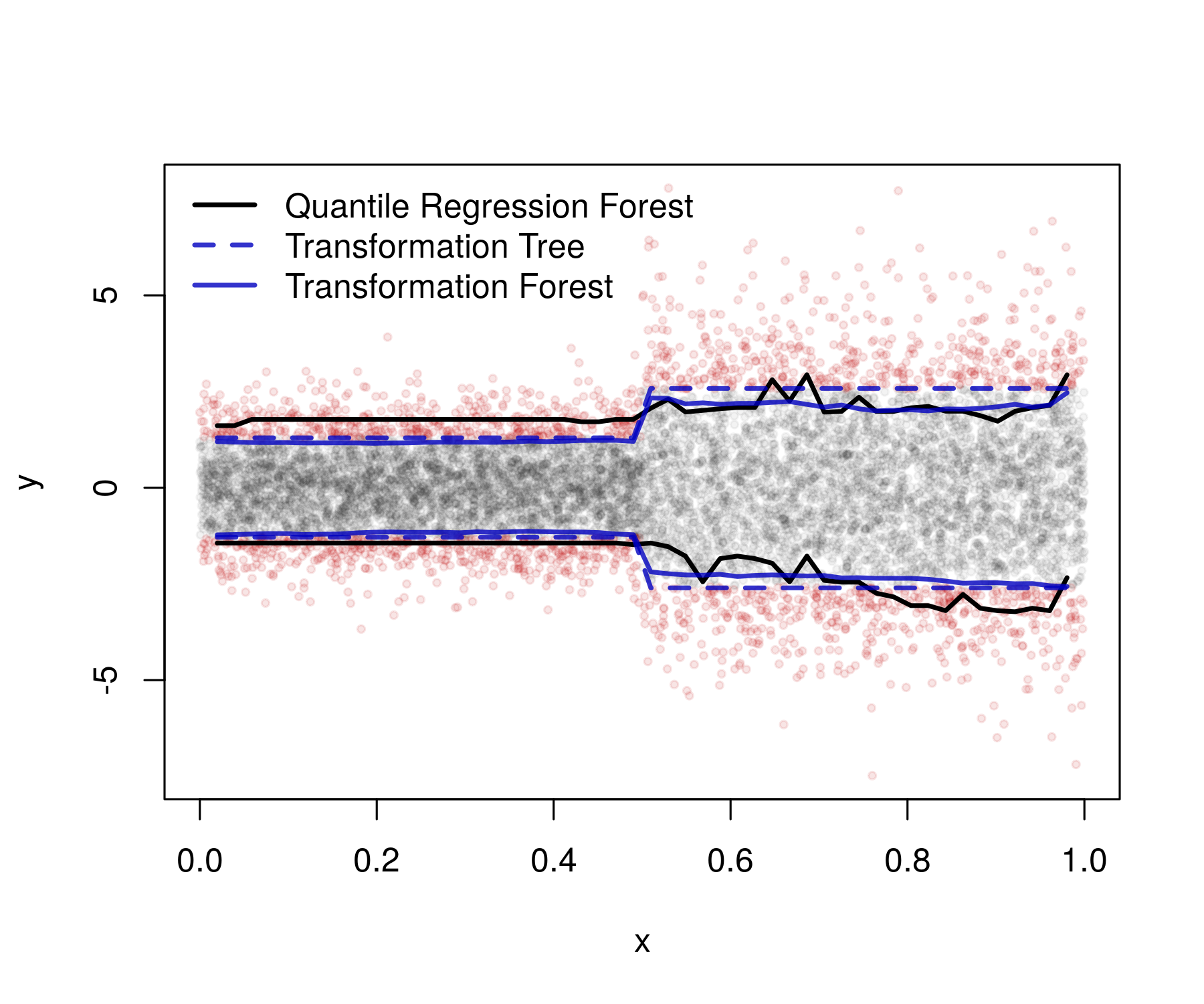
To improve upon quantile regression forests and similar procedures in situations where changes in moments beyond the mean are important, we propose “transformation forests” for the estimation and prediction of conditional distributions for $Y$ given predictor variables $x$ and proceed in three steps. We first suggest to understand forests as adaptive local likelihood estimators (see Bloniarz et al., 2016, for a discussion of the special case of local linear regression). Second, we recap the most important features of the flexible and computationally attractive “transformation family” of distributions (Hothorn et al., 2014; Hothorn et al., 2017) which includes a variety of distribution families. Finally, we adapt the core ideas of “model-based recursive partitioning” (Zeileis et al., 2008, who also provide a review of earlier developments in this field) to this transformation family and introduce novel algorithms for “transformation trees” and “transformation forests” for the estimation of conditional distribution functions which potentially vary in the mean and also in higher moments as a function of predictor variables $x$. In our small example in Figure 1, these novel transformation trees and forests were able to recover the true conditional distributions much more precisely than quantile regression forests.

Owing to the fully parametric nature of the predictive distributions that can be obtained from these novel methods, model inference procedures, such as variable importances, independence tests or model-based resampling, can be formulated in a very general and straightforward way (Section 5). Some remarks on asymptotic properties are given in Section 6. The performance of transformation trees and forests is evaluated empirically on four artificial data generating processes and on survey data for body mass indices from Switzerland in Section 7. Details of the variable and split selection procedure in transformation trees as well as the corresponding theoretical complexity and empirical timings are discussed in Section 8.

We first deal with the unconditional distribution $\mathbb{P}_{Y}$ of a target random variable $Y\in\mathcal{Y}$ and we restrict our attention to a specific probability model defined by the parametric family of distributions

$\displaystyle\mathbb{P}_{Y,\Theta}=\{\mathbb{P}_{Y,\text{\boldmath$\vartheta$}}\mid\text{\boldmath$\vartheta$}\in\Theta\}$

with parameters $\vartheta$ and parameter space $\Theta\subseteq\mathbb{R}^{P}$. With predictors $\text{\boldmath$X$}=(X_{1},\dots,X_{J})\in\mathcal{X}$ from some predictor sample space $\mathcal{X}$, our main interest is in the conditional distribution $\mathbb{P}_{Y\mid\text{\boldmath$X$}=\text{\boldmath$x$}}$ and we assume that this conditional distribution is a member of the family of distributions introduced above, i.e., we assume that a parameter $\text{\boldmath$\vartheta$}(\text{\boldmath$x$})\in\Theta$ exists such that $\mathbb{P}_{Y\mid\text{\boldmath$X$}=\text{\boldmath$x$}}=\mathbb{P}_{Y,\text{\boldmath$\vartheta$}(\text{\boldmath$x$})}$. We call $\text{\boldmath$\vartheta$}:\mathcal{X}\rightarrow\Theta$ the “conditional parameter function” and the task of estimating the conditional distributions $\mathbb{P}_{Y\mid\text{\boldmath$X$}=\text{\boldmath$x$}}$ for all $x$ reduces to the problem of estimating this conditional parameter function.

From the probability model $\mathbb{P}_{Y,\Theta}$ we can derive the log-likelihood contribution $\ell_{i}:\Theta\rightarrow\mathbb{R}$ for each of $N$ independent observations $(y_{i},\text{\boldmath$x$}_{i})$ from the learning sample for $i=1,\dots,N$. We propose and study a novel random forest-type estimator $\text{\boldmath$\vartheta$}^{N}_{\text{Forest}}$ of the conditional parameter function $\vartheta$ in the class of adaptive local likelihood estimators of the form

$\displaystyle\hat{\text{\boldmath$\vartheta$}}^{N}(\text{\boldmath$x$}):=\argmax_{\text{\boldmath$\vartheta$}\in\Theta}\sum_{i=1}^{N}w_{i}^{N}(\text{\boldmath$x$})\ell_{i}(\text{\boldmath$\vartheta$});\quad\text{\boldmath$x$}\in\mathcal{X}$

(1)

where $w_{i}^{N}:\mathcal{X}\rightarrow\mathbb{R}^{+}$ is the “conditional weight function” for observation $i$ given a specific configuration $x$ of the predictor variables (which may correspond to an observation from the learning sample or to new data). This weight measures the similarity of the two distributions $\mathbb{P}_{Y\mid\text{\boldmath$X$}=\text{\boldmath$x$}_{i}}$ and $\mathbb{P}_{Y\mid\text{\boldmath$X$}=\text{\boldmath$x$}}$ under the probability model $\mathbb{P}_{Y,\Theta}$. The main idea is to obtain a large weight for observations $i$ which are “close” to $x$ in light of the model and essentially zero in the opposite case. The superscript $N$ indicates that the weight function may depend on the learning sample, and in fact the choice of the weight function $w_{i}^{N}$ is crucial in what follows.

Local likelihood estimation goes back to Brillinger (1977) in a comment to Stone (1977) and was the topic of Robert Tibshirani’s PhD thesis, published in Tibshirani and Hastie (1987). Early regression models in this class were based on the idea of fitting polynomial models locally within a fixed smoothing window. Adaptivity of the weights refers to an $x$-dependent, non-constant smoothing window, i.e., different weighing schemes are applied in different parts of the predictor sample space $\mathcal{X}$. An overview of local likelihood procedures was published by Loader (1999). Subsequently, we illustrate how classical maximum likelihood estimators, model-based trees, and model-based forests can be embedded in this general framework by choosing suitable conditional weight functions and plugging these into (1).

The unconditional maximum likelihood estimator is based on unit weights $w_{\text{ML},i}^{N}:\equiv 1$ not depending on $x$, i.e., all observations in the learning sample are considered to be equally “close”; thus

$\displaystyle\hat{\text{\boldmath$\vartheta$}}_{\text{ML}}^{N}:=\argmax_{\text{\boldmath$\vartheta$}\in\Theta}\sum_{i=1}^{N}\ell_{i}(\text{\boldmath$\vartheta$}).$

In contrast, model-based trees can adapt to the learning sample by employing rectangular splits to define a partition $\mathcal{X}=\bigcup\limits_{b=1,\dots,B}^{\bullet}\mathcal{B}_{b}$ of the predictor sample space. Each of the $B$ cells then contains a different local unconditional model. More precisely, the conditional weight function $w_{\text{Tree},i}^{N}$ is simply an indicator for $\text{\boldmath$x$}_{i}$ and $x$ being elements of the same terminal node so that only observations in the same terminal node are considered to be “close”. The weight and parameter functions are

$\displaystyle\begin{split}w_{\text{Tree},i}^{N}(\text{\boldmath$x$}):=\sum_{b=1}^{B}I(\text{\boldmath$x$}\in\mathcal{B}_{b}\wedge\text{\boldmath$x$}_{i}\in\mathcal{B}_{b})\\ \hat{\text{\boldmath$\vartheta$}}_{\text{Tree}}^{N}(\text{\boldmath$x$}):=\argmax_{\text{\boldmath$\vartheta$}\in\Theta}\sum_{i=1}^{N}w_{\text{Tree},i}^{N}(\text{\boldmath$x$})\ell_{i}(\text{\boldmath$\vartheta$}).\end{split}$

(2)

Thus, this essentially just picks the parameter estimate from the $b$-th terminal node which is associated with cell $\mathcal{B}_{b}$

$\displaystyle\hat{\text{\boldmath$\vartheta$}}_{b}^{N}=\argmax_{\text{\boldmath$\vartheta$}\in\Theta}\sum_{i=1}^{N}I(\text{\boldmath$x$}_{i}\in\mathcal{B}_{b})\ell_{i}(\text{\boldmath$\vartheta$}),$

along with the corresponding conditional distribution $\mathbb{P}_{Y,\hat{\text{\boldmath$\vartheta$}}_{b}^{N}}$. Model-based recursive partitioning (Zeileis et al., 2008, MOB,) is one representative of such a tree-structured approach.

A forest of $T$ trees is associated with partitions $\mathcal{X}=\bigcup\limits_{b=1,\dots,B_{t}}^{\bullet}\mathcal{B}_{tb}$ for $t=1,\dots,T$. The $b$-th terminal node of the $t$-th tree contains the parameter estimate $\hat{\text{\boldmath$\vartheta$}}_{tb}^{N}$ and the $t$-th tree defines the conditional parameter function $\hat{\text{\boldmath$\vartheta$}}_{\text{Tree},t}^{N}(\text{\boldmath$x$})$. We define the forest conditional parameter function via “nearest neighbour” forest weights

$\displaystyle\begin{split}w_{\text{Forest},i}^{N}(\text{\boldmath$x$}):=\sum_{t=1}^{T}\sum_{b=1}^{B_{t}}I(\text{\boldmath$x$}\in\mathcal{B}_{tb}\wedge\text{\boldmath$x$}_{i}\in\mathcal{B}_{tb})\\ \hat{\text{\boldmath$\vartheta$}}_{\text{Forest}}^{N}(\text{\boldmath$x$}):=\argmax_{\text{\boldmath$\vartheta$}\in\Theta}\sum_{i=1}^{N}w_{\text{Forest},i}^{N}(\text{\boldmath$x$})\ell_{i}(\text{\boldmath$\vartheta$}).\end{split}$

(3)

The conditional weight function $w_{\text{Forest},i}^{N}$ counts how many times $\text{\boldmath$x$}_{i}$ and $x$ are element of the same terminal node in each of the $T$ trees, i.e., captures how “close” the observations are on average across the trees in the forest. Hothorn et al. (2004) first suggested these weights for the aggregation of $T$ survival trees. The same weights have later been used by Lin and Jeon (2006) for estimating conditional means, by Meinshausen (2006) for estimating conditional quantiles and by Bloniarz et al. (2016) for estimating local linear models. An “out-of-bag” version only counts the contribution of the $t$-th tree for observation $i$ when $i$ was not used for fitting the $t$-th tree.

Forests relying on the aggregation scheme (3) model the conditional distribution $\mathbb{P}_{Y\mid\text{\boldmath$X$}=\text{\boldmath$x$}}$ for some configuration $x$ of the predictors as $\mathbb{P}_{Y,\hat{\text{\boldmath$\vartheta$}}_{\text{Forest}}^{N}(\text{\boldmath$x$})}\in\mathbb{P}_{Y,\Theta}$. In this sense, such a forest is a fully specified parametric model with (in-bag or out-of-bag) log-likelihood

$\displaystyle\sum_{i=1}^{N}\ell_{i}\left(\hat{\text{\boldmath$\vartheta$}}_{\text{Forest}}^{N}(\text{\boldmath$x$}_{i})\right)$

allowing a broad range of model inference procedures to be directly applied as discussed in Section 5. Although this core idea seems straightforward to implement, we unfortunately cannot pick our favourite tree-growing algorithm and mix it with some parametric model as two critical problems remain to be addressed in this paper. First, most of the standard tree-growing algorithms are not ready to be used for finding the underlying partitions because their variable and split selection procedures have poor power for detecting distributional changes which are not linked to changes in the mean as was illustrated by the simple toy example presented in the introduction. Therefore, a tailored tree-growing algorithm inspired by model-based recursive partitioning also able to detect changes in higher moments is introduced in Section 4. The second problem is associated with the parametric families $\mathbb{P}_{Y,\Theta}$. Although, in principle, all classical probability models are suitable in this general framework, different parameterizations render unified presentation and especially implementation burdensome. We address this second problem by restricting our implementation to a novel transformation family of distributions. Theoretically, this family contains all univariate probability distributions $\mathbb{P}_{Y}$ and practically close approximations thereof. We highlight important aspects of this family and the corresponding likelihood function in the next section.

A transformation model $\mathbb{P}(Y\leq y)=F_{Y}(y)=F_{Z}(h(y))$ describes the distribution function of $Y$ by an unknown monotone increasing transformation function $h$ and some a priori chosen continuous distribution function $F_{Z}$. We use this framework because simple, e.g., linear, transformation functions implement many of the classical parametric models whereas more complex transformation functions provide similar flexibility as models from the non-parametric world. In addition, discrete and continuous targets, also under all forms of random censoring and truncation, are handled in a unified way. As a consequence, our corresponding “transformation forests” will be applicable to a wide range of targets (discrete, continuous with or without censoring and truncation, counts, survival times) with the option to gradually move from simple to very flexible models for the conditional distribution functions $\mathbb{P}_{Y,\hat{\text{\boldmath$\vartheta$}}_{\text{Forest}}^{N}(\text{\boldmath$x$})}$.

In more detail, let $Z\sim\mathbb{P}_{Z}$ denote an absolutely continuous random variable with density, distribution, and quantile functions $f_{Z}$, $F_{Z}$ and $F^{-1}_{Z}$, respectively. We furthermore assume $0<f_{Z}(z)<\infty\,\forall z\in\mathbb{R}$ for a log-concave density $f_{Z}$ as well as the existence of the first two derivatives of the density $f_{Z}(z)$ with respect to $z$, both derivatives shall be bounded. We do not allow any unknown parameters for this distribution. Possible choices include the standard normal, the standard logistic and the standard minimum extreme value distribution with distribution functions $F_{Z}(z)=\Phi(z)$, $F_{Z}(z)=F_{\SL}(z)=(1+\exp(-z))^{-1}$ and $F_{Z}(z)=F_{\MEV}(z)=1-\exp(-\exp(z))$, respectively.

Let $\mathcal{H}=\{h:\mathcal{Y}\rightarrow\mathbb{R}\mid h(y_{1})<h(y_{2})\,\forall y_{1}<y_{2}\in\mathcal{Y}\}$ denote the space of all strictly monotone transformation functions. With the transformation function $h$ we can write $F_{Y}$ as $F_{Y}(y\mid h)=F_{Z}(h(y))\,\forall y\in\mathcal{Y}$ with density $f_{Y}(y\mid h)$ and there exists a unique transformation function $h=F_{Z}^{-1}\circ F_{Y}$ for all distribution functions $F_{Y}$ (Hothorn et al., 2017). A convenient feature of characterising the distribution of $Y$ by means of the transformation function $h$ is that the likelihood for arbitrary measurements can be written and implemented in an extremely compact form.

For a given transformation function $h$, the likelihood contribution of an observation $y\in\mathbb{R}$ is given by the corresponding density

$\displaystyle\mathcal{L}(h\mid Y=y)=f_{Z}(h(y))h^{\prime}(y).$

The likelihood for intervals $(\underaccent{\bar}{\ry},\bar{y}]\subset\mathcal{Y}$ is, unlike in the above “exact continuous” case, defined in terms of the distribution function (Lindsey, 1996), where one can differentiate between three special cases:

$\displaystyle\mathcal{L}(h\mid Y\in(\underaccent{\bar}{\ry},\bar{y}])=\left\{\begin{array}[]{ll}F_{Z}(h(\bar{y}))-F_{Z}(h(\underaccent{\bar}{\ry}))&y\in(\underaccent{\bar}{\ry},\bar{y}]\quad\text{``interval-censored''}\\ 1-F_{Z}(h(\underaccent{\bar}{\ry}))&y\in(\underaccent{\bar}{\ry},\infty)\quad\text{``right-censored''}\\ F_{Z}(h(\bar{y}))&y\in(-\infty,\bar{y}]\quad\text{``left-censored''}\end{array}\right.$

For truncated observations in the interval $(y_{l},y_{r}]\subset\mathcal{Y}$, the above likelihood contribution has to be multiplied by the factor $(F_{Z}\left(h(y_{r})\right)-F_{Z}\left(h(y_{l})\right))^{-1}$ when $y_{l}<\underaccent{\bar}{\ry}<\bar{y}\leq y_{r}$. A more detailed discussion of likelihood contributions to transformation models can be found in Hothorn et al. (2017).

We parameterise the transformation function $h(y)$ as a linear function of its basis-transformed argument $y$ using a basis function $\text{\boldmath$a$}:\mathcal{Y}\rightarrow\mathbb{R}^{P}$ such that $h(y)=\text{\boldmath$a$}(y)^{\top}\text{\boldmath$\vartheta$},\text{\boldmath$\vartheta$}\in\mathbb{R}^{P}$. In the following, we will write $h=\text{\boldmath$a$}^{\top}\text{\boldmath$\vartheta$}$ and assume that the true unknown transformation function is of this form. For continuous targets $Y$ the parameterisation $h(y)=\text{\boldmath$a$}(y)^{\top}\text{\boldmath$\vartheta$}$ needs to be smooth in $y$, so any polynomial or spline basis is a suitable choice for $a$. For the empirical experiments in Section 7 we employed Bernstein polynomials (Farouki, 2012, for an overview see) of order $M$ ($P=M+1$) defined on the interval $[\underaccent{\bar}{\imath},\bar{\imath}]$ with

	$\displaystyle\text{\boldmath$a$}_{\text{Bs},M}(y)$	$\displaystyle=$	$\displaystyle(M+1)^{-1}(f_{\text{Be}(1,M+1)}(\tilde{y}),\dots,f_{\text{Be}(m,M-m+1)}(\tilde{y}),\dots,f_{\text{Be}(M+1,1)}(\tilde{y}))^{\top}\in\mathbb{R}^{M+1}$
	$\displaystyle h(y)$	$\displaystyle=$	$\displaystyle\text{\boldmath$a$}_{\text{Bs},M}(y)^{\top}\text{\boldmath$\vartheta$}=\sum_{m=0}^{M}\vartheta_{m}f_{\text{Be}(m+1,M-m+1)}(\tilde{y})/(M+1)$
	$\displaystyle h^{\prime}(y)$	$\displaystyle=$	$\displaystyle\text{\boldmath$a$}_{\text{Bs},M}^{\prime}(y)^{\top}\text{\boldmath$\vartheta$}=\sum_{m=0}^{M-1}(\vartheta_{m+1}-\vartheta_{m})f_{\text{Be}(m+1,M-m)}(\tilde{y})M/((M+1)(\bar{\imath}-\underaccent{\bar}{\imath}))$

where $\tilde{y}=(y-\underaccent{\bar}{\imath})/(\bar{\imath}-\underaccent{\bar}{\imath})\in[0,1]$ and $f_{\text{Be}(m,M)}$ is the density of the Beta distribution with parameters $m$ and $M$. This choice is computationally attractive because strict monotonicity can be formulated as a set of $M$ linear constraints on the parameters $\vartheta_{m}<\vartheta_{m+1}$ for all $m=0,\dots,M$ (Curtis and Ghosh, 2011).

The distribution family $\mathbb{P}_{Y,\Theta}=\{F_{Z}\circ\text{\boldmath$a$}^{\top}\text{\boldmath$\vartheta$}\mid\text{\boldmath$\vartheta$}\in\Theta\}$ that transformation forests are based upon is called transformation family of distributions with parameter space $\Theta=\{\text{\boldmath$\vartheta$}\in\mathbb{R}^{P}\mid\text{\boldmath$a$}^{\top}\text{\boldmath$\vartheta$}\in\mathcal{H}\}$ and transformation functions $\text{\boldmath$a$}^{\top}\text{\boldmath$\vartheta$}\in\mathcal{H}$. This family encompasses a wide variety of densities capturing different locations and shapes (including scale and skewness), see Figure 6 for an illustration of different body mass index distributions. The log-likelihood contribution for an observation $y_{i}\in\mathbb{R}$ is now the log-density of the transformation model $\ell_{i}(\text{\boldmath$\vartheta$})=\log(f_{Z}(\text{\boldmath$a$}(y_{i})^{\top}\text{\boldmath$\vartheta$}))+\log(\text{\boldmath$a$}^{\prime}(y_{i})^{\top}\text{\boldmath$\vartheta$})$.

Conceptually, the model-based recursive partitioning algorithm (Zeileis et al., 2008) for tree induction starts with the maximum likelihood estimator $\hat{\text{\boldmath$\vartheta$}}_{\text{ML}}^{N}$. Deviations from such a given model that can be explained by parameter instabilities due to one or more of the predictors are investigated based on the score contributions. The novel “transformation trees” suggested here rely on the transformation family $\mathbb{P}_{Y,\Theta}=\{F_{Z}\circ\text{\boldmath$a$}^{\top}\text{\boldmath$\vartheta$}\mid\text{\boldmath$\vartheta$}\in\Theta\}$ whose score contributions $s$ have relatively simple and generic forms. The score contribution of an “exact continuous” observation $y\in\mathbb{R}$ from an absolutely continuous distribution is given by the gradient of the log-density with respect to $\vartheta$

$\displaystyle\text{\boldmath$s$}(\text{\boldmath$\vartheta$}\mid Y=y)=\text{\boldmath$a$}(y)\frac{f_{Z}^{\prime}(\text{\boldmath$a$}(y)^{\top}\text{\boldmath$\vartheta$})}{f_{Z}(\text{\boldmath$a$}(y)^{\top}\text{\boldmath$\vartheta$})}+\frac{\text{\boldmath$a$}^{\prime}(y)}{{\text{\boldmath$a$}^{\prime}(y)}^{\top}\text{\boldmath$\vartheta$}}.$

For an interval-censored observation $(\underaccent{\bar}{\ry},\bar{y}]$ the score contribution is

$\displaystyle\text{\boldmath$s$}(\text{\boldmath$\vartheta$}\mid Y\in(\underaccent{\bar}{\ry},\bar{y}])=\frac{f_{Z}(\text{\boldmath$a$}(\bar{y})^{\top}\text{\boldmath$\vartheta$})\text{\boldmath$a$}(\bar{y})-f_{Z}(\text{\boldmath$a$}(\underaccent{\bar}{\ry})^{\top}\text{\boldmath$\vartheta$})\text{\boldmath$a$}(\underaccent{\bar}{\ry})}{F_{Z}(\text{\boldmath$a$}(\bar{y})^{\top}\text{\boldmath$\vartheta$})-F_{Z}(\text{\boldmath$a$}(\underaccent{\bar}{\ry})^{\top}\text{\boldmath$\vartheta$})}.$

Under truncation to the interval $(y_{l},y_{r}]\subset\mathcal{Y}$, one needs to substract the term $\text{\boldmath$s$}(\text{\boldmath$\vartheta$}\mid Y\in(y_{l},y_{r}])$ from the score function.

With the transformation model and thus the likelihood and score function being available, we start our tree induction with the global model $\mathbb{P}_{Y,\hat{\text{\boldmath$\vartheta$}}_{\text{ML}}^{N}}$. The hypothesis of all observations $i=1,\dots,N$ coming from this model can be written as the independence of the $P$-dimensional score contributions and all predictors, i.e.,

$\displaystyle H_{0}:\text{\boldmath$s$}(\hat{\text{\boldmath$\vartheta$}}_{\text{ML}}^{N}\mid Y)\perp\text{\boldmath$X$}.$

This hypothesis can be tested either using asymptotic M-fluctuation tests (Zeileis et al., 2008) or permutation tests (Hothorn et al., 2006b; Zeileis and Hothorn, 2013) with appropriate multiplicity adjustment depending on the number of predictors. Rejection of $H_{0}$ leads to the implementation of a binary split in the predictor variable with most significant association to the score matrix; algorithmic details are discussed in Section 8. Unbiasedness of a model-based tree with respect to variable selection is a consequence of splitting in the variable of highest association to the scores where association is measured by the marginal multiplicity-adjusted $p$-value (for details see Hothorn et al., 2006b; Zeileis et al., 2008, and Section 8). The procedure is recursively iterated until $H_{0}$ cannot be rejected. The result is a partition of the sample space $\mathcal{X}=\bigcup\limits_{b=1,\dots,B}^{\bullet}\mathcal{B}_{b}$.

Based on the “transformation trees” introduced here, we construct a corresponding random forest-type algorithm as follows. A “transformation forest” is an ensemble of $T$ transformation trees fitted to subsamples of the learning sample and, optionally, a random selection of candidate predictors available for splitting in each node of the tree. The result is a set of $T$ partitions of the predictor sample space. The transformation forest conditional parameter function is defined by its nearest neighbour forest weights (3).

The question arises how the order $M$ of the parameterisation of the transformation function $h$ via Bernstein polynomials affects the conditional distribution functions $\mathbb{P}_{Y,\hat{\text{\boldmath$\vartheta$}}_{\text{Tree}}^{N}(\text{\boldmath$x$})}$ and $\mathbb{P}_{Y,\hat{\text{\boldmath$\vartheta$}}_{\text{Forest}}^{N}(\text{\boldmath$x$})}$. On the one hand, the basis $\text{\boldmath$a$}_{\text{Bs},1}$ with $F_{Z}=\Phi$ only allows linear transformation functions of a standard normal and thus our models for $\mathbb{P}_{Y\mid\text{\boldmath$X$}=\text{\boldmath$x$}}$ are restricted to the normal family, however, with potentially both mean and variance depending on $x$ as the split criterion in transformation trees is sensitive to changes in both mean and variance. This most simple parameterisation leads to transformation trees and forests from which both the conditional mean and the conditional variance can be inferred. Using a higher order $M$ also allows modelling non-normal distributions. In the extreme case with $M=N-1$ the unconditional distribution function $F_{Z}(\text{\boldmath$a$}_{\text{Bs},M}(y)^{\top}\text{\boldmath$\vartheta$})$ interpolates the unconditional empirical cumulative distribution function of the target. With $M>1$, the split criterion introduced in this section is able to detect changes beyond the second moment and, consequently, also higher moments of the conditional distributions $\mathbb{P}_{Y\mid\text{\boldmath$X$}=\text{\boldmath$x$}}$ may vary with $x$. An empirical comparison of transformation trees and forests with linear ($M=1$) and nonlinear ($M>1$) transformation function can be found in Section 7. Additional empirical properties of transformation models with larger values of $M$ are discussed in Hothorn (2018a).

In contrast to other random forest regression models, a transformation forest is a fully-specified parametric model. Thus, we can derive all interesting model inference procedures from well-defined probability models and do not need to fall back to heuristics. Predictions from transformation models are distributions $\mathbb{P}_{Y,\hat{\text{\boldmath$\vartheta$}}_{\text{Forest}}^{N}(\text{\boldmath$x$})}$ and we can describe these on the scale of the distribution, quantile, density, hazard, cumulative hazard, expectile, and any other characterising functions. By far not being comprehensive, we introduce prediction intervals, a unified definition of permutation variable importance, the model-based bootstrap and a test for global independence in this section.

The theoretical properties of random forest-type algorithms are a contemporary research problem and we refer to Biau and Scornet (2016) for an overview. In this section we discuss how these developments relate to the asymptotic behaviour of transformation trees and transformation forests.

For $\text{\boldmath$\vartheta$}(\text{\boldmath$x$})\equiv\text{\boldmath$\vartheta$}$ the maximum likelihood estimator ($w_{i}\equiv 1$) is consistent and asymptotically normal (Hothorn et al., 2017). In the non-parametric setup, i.e., for arbitrary distributions $\mathbb{P}_{Y}$, Hothorn et al. (2014) provide consistency results in the class of conditional transformation models. Based on these results, consistency and normality of the local likelihood estimator for an a priori known partition $\mathcal{X}=\bigcup\limits_{b=1,\dots,B}^{\bullet}\mathcal{B}_{b}$ is guaranteed as long as the sample size tends to infinity in all cells $b$.

If the partition (transformation trees) or the nearest neighbour weights (transformation forests) are estimated from the data, established theoretical results on random forests (Breiman, 2004; Lin and Jeon, 2006; Meinshausen, 2006; Biau et al., 2008; Biau, 2012; Scornet et al., 2015) provide a basis for the analysis of transformation forests. Lin and Jeon (2006) first analysed random forests for estimating conditional means with adaptive nearest neighbours weights, where estimators for the conditional mean of the form

$\displaystyle\hat{\mathbb{E}}_{N}(Y\mid\text{\boldmath$X$}=\text{\boldmath$x$})=\frac{\sum_{i=1}^{N}w_{\text{Forest},i}^{N}(\text{\boldmath$x$})Y_{i}}{\sum_{i=1}^{N}w_{\text{Forest},i}^{N}(\text{\boldmath$x$})}$

were shown to be consistent in non-adaptive random forests

$\displaystyle\mathbb{E}_{Y\mid\text{\boldmath$X$}=\text{\boldmath$x$}}\left(\mathbb{E}(Y\mid\text{\boldmath$X$}=\text{\boldmath$x$})-\hat{\mathbb{E}}_{N}(Y\mid\text{\boldmath$X$}=\text{\boldmath$x$})\right)^{2}\rightarrow 0$

as $N\rightarrow\infty$. Meinshausen (2006) showed a Glivenko-Cantelli-type result for conditional distribution functions

$\displaystyle\hat{\mathbb{P}}_{N}(Y\leq y\mid\text{\boldmath$X$}=\text{\boldmath$x$})=\hat{\mathbb{E}}_{N}(I(Y\leq y)\mid\text{\boldmath$X$}=\text{\boldmath$x$})=\frac{\sum_{i=1}^{N}w_{\text{randomForest},i}^{N}(\text{\boldmath$x$})I(Y_{i}\leq y)}{\sum_{i=1}^{N}w_{\text{randomForest},i}^{N}(\text{\boldmath$x$})}$

(5)

where the weights are obtained from Breiman and Cutler’s original random forest implementation (Breiman, 2001).

In order to understand the applicability of these results to transformation forests, we define the expected conditional log-likelihood given $x$ for a fixed set of parameters $\vartheta$ as

$\displaystyle\ell(\text{\boldmath$\vartheta$}\mid\text{\boldmath$X$}=\text{\boldmath$x$}):=\mathbb{E}_{Y\mid\text{\boldmath$X$}=\text{\boldmath$x$}}\ell(\text{\boldmath$\vartheta$},Y),$

where $\ell(\text{\boldmath$\vartheta$},Y_{i})=\ell_{i}(\text{\boldmath$\vartheta$})$ is the likelihood contribution by some observation $Y_{i}$. By definition, the true unknown parameter $\text{\boldmath$\vartheta$}(\text{\boldmath$x$})$ has minimal expected risk and thus maximises the expected log-likelihood, i.e.,

$\displaystyle\text{\boldmath$\vartheta$}(\text{\boldmath$x$})=\argmax_{\text{\boldmath$\vartheta$}\in\Theta}\ell(\text{\boldmath$\vartheta$}\mid\text{\boldmath$X$}=\text{\boldmath$x$}).$

Our random forest-type estimator of the expected conditional log-likelihood given $x$ for a fixed set of parameters $\vartheta$ is now

$\displaystyle\hat{\ell}_{N}(\text{\boldmath$\vartheta$}\mid\text{\boldmath$X$}=\text{\boldmath$x$})=\frac{\sum_{i=1}^{N}w_{\text{Forest},i}^{N}(\text{\boldmath$x$})\ell(\text{\boldmath$\vartheta$},Y_{i})}{\sum_{i=1}^{N}w_{\text{Forest},i}^{N}(\text{\boldmath$x$})}.$

Under the respective conditions on the distribution of $X$ and the joint distribution of $Y,\text{\boldmath$X$}$ given by Lin and Jeon (2006), Biau and Devroye (2010), or Biau (2012), this estimator is consistent for all $\text{\boldmath$\vartheta$}\in\Theta$

$\displaystyle\mathbb{E}_{Y\mid\text{\boldmath$X$}=\text{\boldmath$x$}}\left(\ell(\text{\boldmath$\vartheta$}\mid\text{\boldmath$X$}=\text{\boldmath$x$})-\hat{\ell}_{N}(\text{\boldmath$\vartheta$}\mid\text{\boldmath$X$}=\text{\boldmath$x$})\right)^{2}\rightarrow 0$

(the result being derived for non-adaptive random forests). This result gives us consistency of the conditional log-likelihood function

$\displaystyle\hat{\ell}_{N}(\text{\boldmath$\vartheta$}\mid\text{\boldmath$X$}=\text{\boldmath$x$})\stackrel{{\scriptstyle\mathbb{P}}}{{\rightarrow}}\ell(\text{\boldmath$\vartheta$}\mid\text{\boldmath$X$}=\text{\boldmath$x$})\quad\forall\text{\boldmath$\vartheta$}\in\Theta.$

The forest conditional parameter function $\hat{\text{\boldmath$\vartheta$}}_{\text{Forest}}^{N}(\text{\boldmath$x$})$ is consistent when

$\displaystyle\mathbb{P}_{\text{\boldmath$\vartheta$}}(\hat{\ell}_{N}(\text{\boldmath$\vartheta$}_{1}\mid\text{\boldmath$X$}=\text{\boldmath$x$})<\hat{\ell}_{N}(\text{\boldmath$\vartheta$}\mid\text{\boldmath$X$}=\text{\boldmath$x$}))\stackrel{{\scriptstyle\mathbb{P}}}{{\rightarrow}}1$

as $N\rightarrow\infty$ for all $\text{\boldmath$\vartheta$}_{1}$ in a neighbourhood of $\vartheta$. The result $\hat{\text{\boldmath$\vartheta$}}_{\text{Forest}}^{N}(\text{\boldmath$x$})\stackrel{{\scriptstyle\mathbb{P}}}{{\rightarrow}}\text{\boldmath$\vartheta$}(\text{\boldmath$x$})$ can be shown under the assumptions regarding $\ell$ given by Hothorn et al. (2017), especially continuity in $\vartheta$. Because the conditional log-likelihood $\hat{\ell}_{N}(\text{\boldmath$\vartheta$}\mid\text{\boldmath$X$}=\text{\boldmath$x$})$ is a conditional mean-type estimator of a transformed target $Y$, future theoretical developments in the asymptotic analysis of more realistic random forest-type algorithms based on nearest neighbour weights will directly carry over to transformation forests.

It is worth noting that some authors studied properties of random forests in regression models of the form $Y=r(\text{\boldmath$x$})+\varepsilon$ where the conditional variance $\mathbb{V}(Y\mid\text{\boldmath$X$}=\text{\boldmath$x$})$ does not depend on $x$. This is in line with the ANOVA split criterion implemented in Breiman and Cutler’s random forests (Breiman, 2001). The split procedure applied in transformation trees is, as will be illustrated in the next section, able to detect changes in higher moments. Thus, transformation forests might be a way to relax the assumption of additivity of signal and noise in the future.

Transformation forests were evaluated empirically, comparing this novel member of the random forest family to established procedures using artificial data generating processes. The data scenarios controlled the variation of several properties of interest: type of conditional parameter function, types of effect, and model complexity in low and high dimensions. The corresponding hypotheses to be assessed are:

H1:

Type of Conditional Parameter Regression.

H1a:

Tree-Structured Conditional Parameter Function. Transformation trees and forests are able to identify subgroups associated with different transformation models, i.e., subgroups formed by a recursive partition (or tree) in predictor variables $x$ corresponding to different parameters and thus different conditional distributions $\mathbb{P}_{Y\mid\text{\boldmath$X$}=\text{\boldmath$x$}}$.

H1b:

Non-Linear Conditional Parameter Function. Transformation forests are able to identify conditional distributions $\mathbb{P}_{Y\mid\text{\boldmath$X$}=\text{\boldmath$x$}}$ whose parameters depend on predictor variables $x$ in a smooth non-linear way.

H2:

Type of Effect.

H2a:

No Effect. In a non-informative scenario with $\mathbb{P}_{Y\mid\text{\boldmath$X$}=\text{\boldmath$x$}}=\mathbb{P}_{Y}$ (i.e., mean and all higher moments constant) transformation trees perform as good as the unconditional maximum likelihood estimator. Thus, there is no (pronounced) overfitting.

H2b:

Location Only. Transformation trees and forests perform as good as classical regression trees and forests when higher moments of the conditional distribution $\mathbb{P}_{Y\mid\text{\boldmath$X$}=\text{\boldmath$x$}}$ are constant.

H2c:

Unlinked Location and Scale. Transformation trees and forests outperform classical regression trees and forests when higher moments of the conditional distribution $\mathbb{P}_{Y\mid\text{\boldmath$X$}=\text{\boldmath$x$}}$ are varying in a way that is not linked to variations in the mean.

H2d:

Linked Location and Scale. Transformation trees and forests perform as good as classical regression trees and forests when higher moments of the conditional distribution $\mathbb{P}_{Y\mid\text{\boldmath$X$}=\text{\boldmath$x$}}$ are varying but in a way that is linked to the mean.

H3:

Model Complexity.

$P=2$:

Transformation trees and forests with linear transformation function $h$, i.e., with $P=2$ parameters, perform best for conditionally normal target variables. Transformation trees and forests with non-linear transformation function $h$ perform slightly worse in this situation.

$P=6$:

Transformation trees and forests with non-linear transformation function $h$, i.e., with $P=6$ parameters of a Bernstein polynomial of order five, outperform transformation trees and forests with linear transformation function for conditionally non-normal target variables.

H4:

Dimensionality. Transformation forests stabilise transformation trees in the presence of high-dimensional non-informative predictor variables.

The computational complexity of transformation trees and forests basically depends on the variable and split selection performed in every node of the corresponding trees. In this section, we present several possible algorithms for the selection of the “best” binary split and discuss corresponding statistical properties and computational complexities. For a discussion regarding the complexity of random forests we refer to Louppe (2015).

Many prominent tree algorithms, such as CART (Breiman et al., 1984) or C4.5 (Quinlan, 1993) evaluate all possible binary splits in all predictor variables via an exhaustive search. For transformation trees, an exhaustive search

$\displaystyle\hat{\mathcal{B}}=\argmax_{\mathcal{B}\subset\mathcal{X}}\max_{\text{\boldmath$\vartheta$}_{1},\text{\boldmath$\vartheta$}_{2}\in\Theta}\sum_{i=1}^{N}I(\text{\boldmath$x$}_{i}\in\mathcal{B})\ell_{i}(\text{\boldmath$\vartheta$}_{1})+\sum_{i=1}^{N}I(\text{\boldmath$x$}_{i}\in\bar{\mathcal{B}})\ell_{i}(\text{\boldmath$\vartheta$}_{2})$

would require to evaluate the log-likelihood for all possible splits in $O(PN^{2})$. In addition, variable selection based on an exhaustive search would be biased towards variables with many potential splits (Kass, 1980). Unbiased recursive partitioning (Loh and Shih, 1997; Hothorn et al., 2006b; Zeileis et al., 2008, for example) separates variable and split selection to address this bias and to reduce the complexity. Therefore, transformation trees extend the concept of unbiased recursive partitioning by first selecting the most important predictor variable by means of a permutation score test and, in a second step, by finding the best split in this variable as follows (for the sake of simplicity we consider the root node only).

References

- Beran (1988) Beran R (1988). “Prepivoting Test Statistics: A Bootstrap View of Asymptotic Refinements.” Journal of the American Statistical Association, 83(403), 687–697. 10.2307/2289292.
- Biau (2012) Biau G (2012). “Analysis of a Random Forests Model.” Journal of Machine Learning Research, 13(1), 1063–1095. URL http://jmlr.org/papers/v13/biau12a.html.
- Biau and Devroye (2010) Biau G, Devroye L (2010). “On the Layered Nearest Neighbour Estimate, the Bagged Nearest Neighbour Estimate and the Random Forest Method in Regression and Classification.” Journal of Multivariate Analysis, 101(10), 2499–2518. 10.1016/j.jmva.2010.06.019.
- Biau et al. (2008) Biau G, Devroye L, Lugosi G (2008). “Consistency of Random Forests and Other Averaging Classifiers.” Journal of Machine Learning Research, 9, 2015–2033. URL http://jmlr.org/papers/v9/biau08a.html.
- Biau and Scornet (2016) Biau G, Scornet E (2016). “A Random Forest Guided Tour.” Test, 25(2), 197–227. 10.1007/s11749-016-0481-7.
- Bloniarz et al. (2016) Bloniarz A, Wu C, Yu B, Talwalkar A (2016). “Supervised Neighborhoods for Distributed Nonparametric Regression.” In “Proceedings of the 19th International Conference on Artificial Intelligence and Statistics,” pp. 1450–1459. URL http://proceedings.mlr.press/v51/bloniarz16.pdf.
- Breiman (2001) Breiman L (2001). “Random Forests.” Machine Learning, 45(1), 5–32. 10.1023/A:1010933404324.
- Breiman (2004) Breiman L (2004). “Consistency for a Simple Model of Random Forests.” Technical Report 670, Statistics Department, University of California at Berkeley, California. URL http://www.stat.berkeley.edu/~breiman/RandomForests/consistencyRFA.pdf.
- Breiman et al. (2015) Breiman L, Cutler A, Liaw A, Wiener M (2015). Breiman and Cutler’s Random Forests for Classification and Regression. R package version 4.6-12, URL https://CRAN.R-project.org/package=randomForest.
- Breiman et al. (1984) Breiman L, Friedman JH, Olshen RA, Stone CJ (1984). Classification and Regression Trees. Wadsworth, California.
- Brillinger (1977) Brillinger DR (1977). “Discussion of Stone (1977).” The Annals of Statistics, 5(4), 622–623.
- Bundesamt für Statistik (2013) Bundesamt für Statistik (2013). Die Schweizerische Gesundheitsbefragung 2012 in Kürze – Konzept, Methode, Durchführung. Bern. URL http://www.bfs.admin.ch.
- Criminisi et al. (2012) Criminisi A, Shotton J, Konukoglu E (2012). “Decision Forests: A Unified Framework for Classification, Regression, Density Estimation, Manifold Learning and Semi-Supervised Learning.” Foundations and Trends in Computer Graphics and Vision, 7(2–3), 81–227. 10.1561/0600000035.
- Curtis and Ghosh (2011) Curtis SM, Ghosh SK (2011). “A Variable Selection Approach to Monotonic Regression with Bernstein Polynomials.” Journal of Applied Statistics, 38(5), 961–976. 10.1080/02664761003692423.
- Efron and Tibshirani (1993) Efron B, Tibshirani RJ (1993). An Introduction to the Bootstrap. Chapman & Hall, New York.
- Farouki (2012) Farouki RT (2012). “The Bernstein Polynomial Basis: A Centennial Retrospective.” Computer Aided Geometric Design, 29(6), 379–419. 10.1016/j.cagd.2012.03.001.
- Foster et al. (2011) Foster JC, Taylor JM, Ruberg SJ (2011). “Subgroup Identification from Randomized Clinical Trial Data.” Statistics in Medicine, 30(24), 2867–2880. 10.1002/sim.4322.
- Friedman (1991) Friedman JH (1991). “Multivariate Adaptive Regression Splines.” The Annals of Statistics, 19(1), 1–67.
- Gneiting et al. (2007) Gneiting T, Balabdaoui F, Raftery AE (2007). “Probabilistic Forecasts, Calibration and Sharpness.” Journal of the Royal Statistical Society B, 69(2), 243–268. 10.1111/j.1467-9868.2007.00587.x.
- Gneiting and Raftery (2007) Gneiting T, Raftery AE (2007). “Strictly Proper Scoring Rules, Prediction, and Estimation.” Journal of the American Statistical Association, 102(477), 359–378. 10.1198/016214506000001437.
- Hapfelmeier et al. (2014) Hapfelmeier A, Hothorn T, Ulm K, Strobl C (2014). “A New Variable Importance Measure for Random Forests with Missing Data.” Statistics and Computing, 24(1), 21–34. 10.1007/s11222-012-9349-1.
- Hothorn (2017a) Hothorn T (2017a). mlt: Most Likely Transformations. R package version 0.2-2, URL http://CRAN.R-project.org/package=mlt.
- Hothorn (2017b) Hothorn T (2017b). Most Likely Transformations: The mlt Package. R package vignette version 0.2-1, URL https://CRAN.R-project.org/package=mlt.docreg.
- Hothorn (2018a) Hothorn T (2018a). “Top-Down Transformation Choice.” Statistical Modelling. URL https://arxiv.org/abs/1706.08269.
- Hothorn (2018b) Hothorn T (2018b). Transformation Trees and Forests. R package version 0.3-0, URL https://CRAN.R-project.org/package=trtf.
- Hothorn et al. (2006a) Hothorn T, Hornik K, van de Wiel MA, Zeileis A (2006a). “A Lego System for Conditional Inference.” The American Statistician, 60(3), 257–263. 10.1198/000313006X118430.
- Hothorn et al. (2006b) Hothorn T, Hornik K, Zeileis A (2006b). “Unbiased Recursive Partitioning: A Conditional Inference Framework.” Journal of Computational and Graphical Statistics, 15(3), 651–674. 10.1198/106186006X133933.
- Hothorn et al. (2014) Hothorn T, Kneib T, Bühlmann P (2014). “Conditional Transformation Models.” Journal of the Royal Statistical Society: Series B (Statistical Methodology), 76(1), 3–27. 10.1111/rssb.12017.
- Hothorn et al. (2004) Hothorn T, Lausen B, Benner A, Radespiel-Tröger M (2004). “Bagging Survival Trees.” Statistics in Medicine, 23(1), 77–91. 10.1002/sim.1593.
- Hothorn et al. (2017) Hothorn T, Möst L, Bühlmann P (2017). “Most Likely Transformations.” Scandinavian Journal of Statistics. 10.1111/sjos.12291.
- Hothorn and Zeileis (2015) Hothorn T, Zeileis A (2015). “partykit: A Modular Toolkit for Recursive Partytioning in R.” Journal of Machine Learning Research, 16, 3905–3909. URL http://jmlr.org/papers/v16/hothorn15a.html.
- Hothorn and Zeileis (2017) Hothorn T, Zeileis A (2017). partykit: A Toolkit for Recursive Partytioning. R package version 1.2-0, URL https://CRAN.R-project.org/package=partykit.
- Ishwaran et al. (2008) Ishwaran H, Kogalur UB, Blackstone EH, Lauer MS (2008). “Random Survival Forests.” The Annals of Applied Statistics, 2(3), 841–860. 10.1214/08-aoas169.
- Kass (1980) Kass GV (1980). “An Exploratory Technique for Investigating Large Quantities of Categorical Data.” Journal of the Royal Statistical Society. Series C (Applied Statistics), 29(2), 119–127. 10.2307/2986296.
- Lin and Jeon (2006) Lin Y, Jeon Y (2006). “Random Forests and Adaptive Nearest Neighbors.” Journal of the American Statistical Association, 101(474), 578–590. 10.1198/016214505000001230.
- Lindsey (1996) Lindsey JK (1996). Parametric Statistical Inference. Clarendon Press, Oxford.
- Loader (1999) Loader C (1999). Local Regression and Likelihood. Springer-Verlag, New York.
- Loh and Shih (1997) Loh WY, Shih YS (1997). “Split Selection Methods for Classification Trees.” Statistica Sinica, 7, 815–840.
- Lohse et al. (2017) Lohse T, Rohrmann S, Faeh D, Hothorn T (2017). “Continuous Outcome Logistic Regression for Analyzing Body Mass Index Distributions.” F1000Research, 6, 1933. 10.12688/f1000research.12934.1.
- Louppe (2015) Louppe G (2015). “Understanding Random Forests: From Theory to Practice.” Technical report, arXiv 1407.7502, v3. URL http://arxiv.org/abs/1510.04342.
- Mayr et al. (2012) Mayr A, Hothorn T, Fenske N (2012). “Prediction Intervals for Future BMI Values of Individual Children–A Non-Parametric Approach by Quantile Boosting.” BMC Medical Research Methodology, 12, 6. 10.1186/1471-2288-12-6.
- McLachlan (1987) McLachlan GL (1987). “On Bootstrapping the Likelihood Ratio Test Stastistic for the Number of Components in a Normal Mixture.” Journal of the Royal Statistical Society. Series C (Applied Statistics), 36(3), 318–324.
- Meinshausen (2006) Meinshausen N (2006). “Quantile Regression Forests.” Journal of Machine Learning Research, 7, 983–999. URL http://jmlr.org/papers/v7/meinshausen06a.html.
- Meinshausen (2017) Meinshausen N (2017). quantregForest: Quantile Regression Forests. R package version 1.3-7, URL https://CRAN.R-project.org/package=quantregForest.
- Moradian et al. (2016) Moradian H, Larocque D, Bellavance F (2016). “ Splitting Rules in Survival Forests.” Lifetime Data Analysis. 10.1007/s10985-016-9372-1.
- Quinlan (1993) Quinlan RR (1993). C4.5: Programs for Machine Learning. Morgan Kaufmann Publishers, San Francisco, California.
- R Core Team (2016) R Core Team (2016). R: A Language and Environment for Statistical Computing. R Foundation for Statistical Computing, Vienna, Austria. URL https://www.R-project.org/.
- Scornet et al. (2015) Scornet E, Biau G, Vert JP (2015). “Consistency of Random Forests.” The Annals of Statistics, 43(4), 1716–1741. 10.1214/15-AOS1321.
- Seibold et al. (2016) Seibold H, Zeileis A, Hothorn T (2016). “Model-Based Recursive Partitioning for Subgroup Analyses.” International Journal of Biostatistics, 12(1), 45–63. 10.1515/ijb-2015-0032.
- Seibold et al. (2017) Seibold H, Zeileis A, Hothorn T (2017). “Individual Treatment Effect Prediction for ALS Patients.” Statistical Methods in Medical Research. 10.1177/0962280217693034.
- Stone (1977) Stone CJ (1977). “Consistent Nonparametric Regression (with Discussion).” The Annals of Statistics, 5(4), 595–645. 10.1214/aos/1176343886.
- Strasser and Weber (1999) Strasser H, Weber C (1999). “On the Asymptotic Theory of Permutation Statistics.” Mathematical Methods of Statistics, 8, 220–250. Preprint available from http://epub.wu-wien.ac.at/dyn/openURL?id=oai:epub.wu-wien.ac.at:epub-wu-01_94c.
- Strobl et al. (2008) Strobl C, Boulesteix AL, Kneib T, Augustin T, Zeileis A (2008). “Conditional Variable Importance for Random Forests.” BMC Bioinformatics, 9(307). 10.1186/1471-2105-9-307.
- Strobl et al. (2007) Strobl C, Boulesteix AL, Zeileis A, Hothorn T (2007). “Bias in Random Forest Variable Importance Measures: Illustrations, Sources and a Solution.” BMC Bioinformatics, 8, 25. 10.1186/1471-2105-8-25.
- Tibshirani and Hastie (1987) Tibshirani R, Hastie T (1987). “Local Likelihood Estimation.” Journal of the American Statistical Association, 82(398), 559–567. 10.1080/01621459.1987.10478466.
- Wager and Athey (2017) Wager S, Athey S (2017). “Estimation and Inference of Heterogeneous Treatment Effects Using Random Forests.” Journal of the American Statistical Association. URL http://arxiv.org/abs/1510.04342.
- Zeileis and Hothorn (2013) Zeileis A, Hothorn T (2013). “A Toolbox of Permutation Tests for Structural Change.” Statistical Papers, 54(4), 931–954. 10.1007/s00362-013-0503-4.
- Zeileis et al. (2008) Zeileis A, Hothorn T, Hornik K (2008). “Model-Based Recursive Partitioning.” Journal of Computational and Graphical Statistics, 17(2), 492–514. 10.1198/106186008X319331.
Appendix
Computational Details
A reference implementation of transformation trees and transformation forests is available in the \pkgtrtf package (Hothorn, 2018b). This package was built on top of the infrastructure packages \pkgpartykit (Hothorn and Zeileis, 2015; Hothorn and Zeileis, 2017) and \pkgmlt (Hothorn, 2017a; Hothorn, 2017b). Conditional inference trees and forests were fitted using package \pkgpartykit. Quantile regression forests were computed by the \pkgquantregForest package (Meinshausen, 2017). The reference implementation of Breiman’s and Cutlers random forests in the \pkgrandomForest package (Breiman et al., 2015) was used. All computations were performed using R version 3.4.3 (R Core Team, 2016).
For the empirical evaluation in Section 7, all non-linear transformation models were based on transformation functions parameterised in terms of Bernstein polynomials of order five, i.e., with six parameters, and . Log-likelihoods were optimised under monotonicity constraints using a combination of augmented Lagrangian minimisation and spectral projected gradients. Unbiased trees, including transformation trees, stopped internally when the minimum Bonferroni-adjusted -value was larger than . No such internal stopping was applied in conditional inference or transformation forests. Subsampling of observations was used for all random forest-types. The minimum number of observations necessary for splitting (minsplit in \pkgpartykit and nodesize in \pkgrandomForest) was for all forest types in the simulation experiments.
Data from the Swiss Health Survey 2012 can be obtained from the Swiss Federal Statistics Office (Email: sgb12@bfs.admin.ch). Data is available for scientific research projects, and a data protection application form must be submitted. More information can be found here http://www.bfs.admin.ch/bfs/de/home/statistiken/gesundheit/erhebungenSupplementary. The code used for producing the results for the body mass illustration can be evaluated on a smaller artificial data set sampled from the transformation forest by running demo("BMI") from the \pkgtrtf package (Hothorn, 2018b); Figure 1 is regenerated by demo("QRF"). The simulation results presented in this paper can be reproduced using the files in system.file("sim", package = "trtf").
Additional Results: Empirical Evaluation
Additional Evaluation of Tree-Structured Conditional Parameter Function (H1a)
Additional Evaluation of Non-Linear Conditional Parameter Function (H1b)
Review History: Version 1 by Journal 1 (January 2017–May 2017)
Review for version 1 (https://arxiv.org/abs/1701.02110v1). Comments by referees are printed in italics, replies by the authors in plain text.
Handling Editor
Both reports find the paper interesting in that it combines partitioning methods with local likelihood estimation. However, they also raise very good questions about the paper. I have also taken a look at the paper myself. I highlight the important points/issues below, combining the reports’ comments and my own:
- 1.
Computational complexity of the proposed method, especially in high-dimension, needs to be addressed.
We added a new Section 8 containing a detailed description of the variable and split selection methods in transformation trees. This section also discusses the statistical properties and the computational complexity of these variants. The theoretical findings are supported by an analysis of the empirical runtimes.
- 2.
Reproducibility of the experimental results is unclear. That is, the simulation set-ups are not clear enough for a reader to reproduce the results by writing their own codes. Please make the results reproducible.
GPL-2 licensed open-source code implementing transformation trees and forests is available from CRAN since 2018-01-08 (package trtf). The revision now contains a link to the source code for the artificial simulation experiments. Reproducibility material for the body weight application is published with Hothorn (2018). These issues are discussed in Section “Computational Details”.
- 3.
A much clearer description is needed on how your proposed method is built on existing works in the literature, and please cite all appropriate papers (the second report mentions a few more).
We agree that the description of unbiased model-based recursive partitioning was a little too opague in the first version. We comment on statistics used for variable and split selection in unbiased model-based recursive partitioning (and thus also by transformation trees) now in much more detail in our new Section 8.
- 4.
More explanation and evidence on why a new method like yours is needed too, given the many related method – I understand that interpretability is a motivation, did you illustrate clearly the interpretability of your new method in the data example?
We believe that the new simulation experiments support our main hypothesis that none of the existing tree or forest algorithms is able to detect distributional changes unrelated to the mean. Transformation trees and forests fill this gap. This fact is prominently stated in the introduction and throughout the manuscript and motivated the design of the new simulation experiments. The new illustration regarding body weight gives an (as we hope) easy to understand impression of how transformation trees and forests detect and represent distributional changes in higher moments of the conditional distribution of the target given predictor variables.
- 5.
Computational complexity comparisons to representatives of the existing methods, including in terms of running times of your method and others in the experimental results section.
See point 1.
- 6.
Since RF is commonly used in practice rather than the model-based partitioning method, it is necessary to use one version of RF, for example, the one by Breiman, in place of the model-based partitioning method, to generate weights used in the proposed method. Comparisons to this RF-based version of the proposed methods in terms of computational complexity (running time) and prediction and confidence interval metrics are needed.
We agree that most readers will be interested in a direct comparison with Breiman and Cutler’s randomForests. The new simulation experiments directly compare transformation trees and forests as well as conditional inference trees and forests with this reference implementation of random forests. We followed the suggestion to estimate a conditional transformation model based on weights extracted from Breiman and Cutler’s randomForests. Therefore, a direct comparison to transformation forests on the same scale is now presented. Prediction error is assessed based on the out-of-sample log-likelihood and prediction intervals are evaluated based on the and check risk. Theoretical and empirical runtimes are studied in our new Section 8.
- 7.
Moreover, I am not convinced that model-based bootstrap is a good method to use for uncertainty measures, especially in high-dim and when the data generating model is misspecified or is a mis-match for the parametric models used in your method.
We did not evaluate the quality of the model-based bootstrap (Section 5.3) nor size and power of the likelihood-ratio test (Section 5.4) in the initial submission. The main point we were trying to make in Section 5 was that the understanding of transformation forests as parametric models allows such procedures to be implemented. The model-based bootstrap for the approximation of the null distribution of likelihood-ratio statistics was introduced already in the late 1980ies (two references were added). Its size of course depends on how well the null model describes the data and how much the transformation forest overfits the data. We investigate the latter issue in the new artificial simulation experiments in Section 7, also in the presence of non-informative predictor variables. We now explicitly mention (in the discussion) that an empirical evaluation of likelihood-based variable importances for variable selection, the model-based bootstrap for variability assessment and of the likelihood-ratio test are ongoing research projects.
Reviewer 1
Your general framework is very clear, it is a good idea, and it fits very well into results which already exist about random forest.
Thank you!
You are splitting the space in such a way that the second expression on page 8 is maximized.
We regret the confusion caused by the second formula on page 8, which suggested that an exhaustive search is performed. Unbiased recursive partitioning avoids exhaustive evaluations of all potential splits by a separation of variable and split selection. The formula was understood as an illustration of the concept, not the actual implementation. We moved this formula to Section 8 and added a much more detailed description of variable and split selection in transformation trees.
If I understand that correctly, then you approximate the true likelihood by the “exact continuous” approximation instead of the correct likelihood function as on page 6. I can see that this can make sense when the partitions are very small. But isn’t that a problem in the beginning when the partition is very big or in high dimensions? Is there a computational reason for doing this? Have you done simulations, how that choice affects the performance of your estimator?
We are sorry for the insufficient description of the different likelihood contributions. The “approximation” of the “exact” likelihood by the density is a rather uncommon (at least outside survival analysis) concept. However, the theory of transformation models is closely tied to the understanding and evaluation of the “exact” likelihood for interval-censored observations. Because we can never observe real numbers (only intervals), we felt it would help to think of the “exact” likelihood as a probability (the definition by Fisher dating back to 1922 in fact advocates this point of view). We rephrased this paragraph and separately introduce the likelihood for real numbers and intervals now. The new Section 8 also introduces a potential application of the interval-censored likelihood as a means for reducing runtimes of the algorithm.
In general, I wonder to what extend the argmax on page 8 is realizable? That seems quite costly to me. The best split in random forest can be found in O(p * n * log(n)). How does this expression compare, if you only consider axis-aligned slits of p features with n possible splitting points? It would be nice to see an expression of the computational complexity and a runtime comparison in terms of n and p.
You are right, of course. We discuss theoretical and empirical runtimes in more detail in our new Section 8.
Furthermore, the score function is used as a pruning criteria which totally makes sense for single regression trees, but in the standard Random Forest, people usually do not do such pruning. Have you considered not to implement this pruning criterion? One could perform splits until at least k observations are left in each leaf. Wouldn’t that speed up the simulation? Your random forest version could perform better.
We apologise for not being more precise in the description of our implementation of transformation forests. Of course, forests aggregate over trees built without internal stopping. For transformation trees it makes sense to restrict terminal nodes to a certain number of observations because it won’t be possible to estimate the parameters of the transformation model (and thus to compute the score matrix) with being too small. Because the size of a terminal node cannot be controlled directly in the randomForest package (the parameter nodesize corresponds to minsplit but not minbucket in rpart or partykit terminology), we required at least observations in order to implement a split for all forest variants under test.
For the parametric bootstrap, why would you throw away those “extreme” samples? That can make sense, but throwing them away would not be the parametric bootstrap, and there is some intuition which I might be missing.
You are right, the distribution of the likelihood ratio statistic is not the only bootstrap distribution one could be interested in. We replaced this paragraph explaining that one can look at the bootstrap distribution of the parameters or any functional thereof (including the LR statistic).
I wonder whether this is the right Likelihood-Ratio Test. What if the true distribution is independent of , but it is very complicated and cannot be approximated by your unconditional maximum likelihood model. Then your original statistics has a completely different distribution than your simulated H0 distribution, and you might falsely reject , right?
Of course. We clarified (in Section 2, see also point “p.6, l.-4” by referee 2) that we assume that the true transformation function can be written as throughout the manuscript. Under this condition, the procedure is just the simple parametric bootstrap. See also point 7 by the editor.
Furthermore, it would also be nice to have an intuitive statement of how the choice of the set in which lies affects the bias-variance trade-off.
We explicitly cover this point in the empirical evaluations in Section 7 now. The empirical effects of using the ‘correct’ transformation function (for example, a linear function for conditionally normal targets) compared to an overparameterised (ie, non-linear) version are investigated in a simulation model with normal targets. For log-normal targets, the loss of using an underparameterised (linear) transformation function is also presented.
- 8.
The way I understand your simulation setup is the following: You take real data sets, you fit each method, and then you use the parametric bootstrap to create from each fitted estimator new data sets. Those new data sets have the same feature points but values created from the fitted models. To compare with fully non-parametric estimators (such as quantile regression forest) wouldn’t it make more sense to use a bigger data set, use on one part of it as a training data set and use the rest as an evaluation data set? At least for confidence intervals comparisons that would be very appealing to me and it would be fair since all of your models are essentially based on transformation models, right? If you need access to the true underlying data generating process, it might be worthwhile also comparing your methods to made up data generating processes. Otherwise, you are comparing four estimators with QRF by creating data directly coming from models which are generated by those estimators.
Our intention was to evaluate the methods based on “realistic” simulation models related to a specific algorithm. We think that our comparison with quantile regression forests were correct, because we also directly sampled (nonparametrically) from this model. The main problem with a bootstrap-based simulation is that the “simulation model” is a tree or a forest and only the former can be visualised and directly understood. We also understand the points you and the other reviewer raised and therefore implemented a more traditional simulation study based on artificial data generating processes with separate learning and validation sets in Section 7.
- 9.
There is also an estimator called Density Forest and Manifold Forest, which were for example mentioned in Criminisi et al. 2011. It would be nice to have a comparison to those methods as well.
Thank you very much for pointing us to this interesting publication. Our understanding of http://dx.doi.org/10.1561/0600000035 (page 134) is that the model is conditional normal with predictor-dependent mean and variance. However, it is unclear (in this and other publications from the group) how the underlying trees handle variance heterogeneity that can be explained by the predictor variables (no details regarding the “weak learner” are presented on page 137). The more flexible (as it seems) density and manifold forests are for the unsupervised case only.
The authors provide software for reproducing results presented in a follow-up book (“Sherwood” from https://www.microsoft.com/en-us/download/details.aspx?id=52340&751be11f-ede8-5a0c-058c-2ee190a24fa6=True).
{Schunk}{Sinput}> set.seed(290875) > N <- 1000 > x <- runif(N, min = -1, max = 1) > y <- rnorm(N, mean = sin(2 * x * pi), sd = exp(x)) > plot(y x) > write.table(data.frame(x = x, y = y), file = "th.txt", + col.names = FALSE, row.names = FALSE, sep = ""͡)
Figure 22: Example to be used for “Sherwood” example code. We generated an example data set (Figure 22) and tried to run the software on this example using
./sw regression /t 100 /d 10 th.txt
and obtained the following output
Training the forest...
Trained 100 trees.
Applying the forest to test data...
Applied 100 trees.
Segmentation fault (core dumped)
It also seems that the only output the software can produce is a bitmap file with the original data overlayed with the model. We did not find any possibility to specify test data, let alone a means to compute out-of-sample prediction errors etc. For these reasons it was not possible for us to include this implementation as an additional competitor in the empirical evaluations in Section 7. However, the method is interesting because mean aggregation of conditional densities is performed, and this is similar to the mean aggregation of cumulative hazard functions in random survival forests. The introduction now highlights this similarity.
- 10.
For you confidence interval simulations, there are two things to consider. They should have the correct coverage, and they should be small. I would also be curious how your confidence intervals differ in size.
It is in general hard to compare prediction intervals, because they condition on a specific set of predictor variables. Thus, coverage and lengths can differ substantially over the sample space. We elaborate on this issue in Section 7 and also point to the proper scoring rules literature. However, the check risk for the and quantiles is appropriate to compare the ability of methods to estimate these conditional quantiles and we, in addition to the negative log-likelihood and the absolute error, report these two performance measures.
Little typos: (omitted). Thank you, we silently corrected the typos.
Reviewer 2
Overview
This is an interesting paper. Hothorn and Zeileis describe using weights, say derived from a random forest algorithm to fit the model: