A Theory of Solvability for Lossless Power Flow Equations – Part II: Conditions for Radial NetworksThanks: J. W. Simpson-Porco is with the Department of Electrical and Computer Engineering, University of Waterloo. Email: jwsimpson@uwaterloo.ca.

We leverage the FPPF developed in Part I, and for radial networks we derive sufficient conditions which ensure the power flow equations possess a solution. Our conditions guarantee the existence of a solution within a desirable set in voltage space, where voltage magnitudes are near their open-circuit values and phase angle differences between buses are small. For simplified topologies containing no connections between PQ buses, we further show that our existence condition implies the fixed-point power flow mapping $f$ is a contraction mapping. This in turn implies that (i) the solution is unique within the specified set, and (ii) the FPPF iteration $v_{k+1}=f(v_{k})$ converges exponentially to the unique power solution. For certain cases, we show our conditions are also necessary for existence. As a byproduct of our analysis, we also establish the non-existence of solutions within both a “medium-voltage” and an ”extra-high-voltage” region of voltage-space. The existence of this medium-voltage solutionless region implies a lower bound in voltage-space between the unique high-voltage solution and any undesirable low-voltage solutions.

The conditions we derive are parametric, depending only on the given data of the power flow problem including fixed active and reactive power injections, shunt and series susceptances, the network topology, and PV bus voltage set-points. Rather than imposing spectral or worst-case bounds individually on these quantities, our conditions fuse the relevant parameters together into intuitive loading margins for the system, by exploiting the stiffness matrices introduced in Part I [1, Def. 2]. These loading margins generalize the textbook two-bus network feasibility results [2, Chapter 2], and unify recent results on feasibility of decoupled active [3] and reactive [4] power flow. While our results are currently restricted to an unrealistic class of networks (lossless, radial), the analysis presented is — in the authors opinion — the most complete one available in the literature. The theoretical results here also provide a partial explanation for the robust numerical behavior of the FPPF iteration observed in Part I.

Section II presents an extensive literature review, surveying the history of power flow solvability results, with a focus on incorporating structural information into solvability conditions.

Section III briefly reviews the grid model, then presents a detailed analysis of the classic two-bus model of power flow between a PQ bus and a PV bus, providing context for our network generalizations. Section IV briefly re-states the required definitions and notation for the FPPF model.

In Section V we state and prove our main results on the existence and uniqueness of power flow solutions. The proof is technical; casual readers will wish to simply read the theorem statements along with the explanations which follow them. Section VI concludes and lists some open problems.

We refer the reader to Part I [1] for notational conventions.

Fixed Point Theory: A point $x^{*}\in\mathbb{R}^{n}$ is a fixed point of a map $f:\mathbb{R}^{n}\rightarrow\mathbb{R}^{n}$ if $f(x^{*})=x^{*}$. A set $\mathcal{X}\subset\mathbb{R}^{n}$ is invariant for $f$ if $x\in\mathcal{X}\Rightarrow f(x)\in\mathcal{X}$. If $\mathcal{X}$ is a compact, convex, and invariant set for $f$, then $f$ possess at least one fixed point $x^{*}\in\mathcal{X}$ [5, Section 7, Corollary 8]. We say $f$ is a contraction map on $\mathcal{X}$ if there exists a $\beta\in{[0,1)}$ (the contraction rate) and a vector norm $\|\cdot\|$ such that for any $x,y\in\mathcal{X}$, $\|f(x)-f(y)\|\leq\beta\|x-y\|$. If $f$ is a contraction map on an invariant compact set $\mathcal{X}$, then $f$ has a unique fixed point $x^{*}\in\mathcal{X}$ [6, Theorem 9.32], and the iterates of $x_{k+1}=f(x_{k})$ of $f$ from any initial point $x_{0}\in\mathcal{X}$ satisfy $\|x_{k}-x^{*}\|\leq\beta^{k}\|x_{0}-x^{*}\|$.

Korsak [7] appears to be among the first to explicitly study the solution space of power flow equations and, in the context of swing stability, constructed an example showing that decoupled active power flow can possess multiple “stable” solutions in meshed networks. Simultaneously, Tavora and Smith [8] studied those same equations, giving a necessary condition for solvability and studying the singular surfaces of the active power flow Jacobian for low-dimensional systems. A more detailed study of decoupled active power flow was later performed by Araposthatis, Sastry and Varaiya [9, 10]. Galiana and Jarjis [11, 12, 13] investigated the coupled equations in rectangular coordinates, proposing feasibility conditions based on supporting hyperplanes for a generalized injection region in parameter-space. Unfortunately the assumption that the injection region is a convex cone was later shown to be incorrect; see, for example, [14, 15, 16, 17]. Soon after, Baillieul and Byrnes [18] leveraged geometric techniques to provide a combinatorial upper bound on the number of complex solutions; for particularly clear expositions on the nature of multiple solutions, see the articles [19, 20, 21].

Wu was the first to apply the fixed point and degree techniques developed for nonlinear circuits to power flow [22]. In two breakthrough papers [23, 24], Wu and Kumagai applied the Leray-Schauder fixed point theorem to derive conditions for solvability of both the decoupled active and reactive power flow equations. Using homotopy and degree theory, they showed that under some additional conditions, the coupled power flow equations also possess a solution. In a similar spirit, Thorp, Schulz and Ilić [25, 26] later applied nonlinear circuit results to derive a conservative condition for solvability of decoupled reactive power flow. In [27] Chiang and Baran studied feasibility on distribution feeders using Baran’s branch flow model, arguing in a quasi-quantitative manner that the system has a unique solution. Unfortunately the arguments provided no quantitative bounds. Grijalva and Sauer [28, 29] proposed necessary conditions for Jacobian singularity based on the saturation of transmission lines. In [30] Lesieutre, Sauer, and Pai derived sufficient solvability conditions, but the analysis forbids constant power loads. In [31] voltage magnitudes were isolated in terms of voltage phase angles, yielding a semi-explicit power flow solution, but the analysis is restricted to impedance load models.

While little progress was made through the 2000s, a recent flurry of activity has yielded new results. In [3, 32] Dörfler et al. noted that the decoupled active power flow in polar form could be exactly solved on acyclic networks, leading them to an explicit necessary and sufficient condition for existence and uniqueness. The condition was also shown to also be tight for networks with short cycles, and a conservative sufficient condition was given for general meshed networks; see also [33]. Barabanov et al. proposed a necessary condition for LTI systems with constant power loads [34]. Molzahn et al. proposed a necessary condition for the coupled lossy power flow problem. In [4] the author and his collaborators derived a sufficient condition for solvability of decoupled reactive power flow, analogous to the active power flow results in [3]. For distribution feeders, Bolognani and Zampieri [35] reformulated the complex-valued power flow as a fixed point mapping, and derived a condition under which there exists a unique solution, with a relaxed condition proposed later by Yu et al. in [36], and further distribution system results in [37, 38].

As a complement to fixed point-based approaches, convexity has emerged as a powerful tool for analyzing power flow solvability. In the context of optimal power flow, sufficient conditions have been found for both radial and meshed networks under which various convex relaxations are exact; see [39, 40] for a broad survey of recent results. The implication is that under such conditions, convex programming can be used to iteratively find the solution, or otherwise certify that no solution exists. Inspired by classical work on transient stability, Dvijotham et al. have pursued the energy-function formulation of lossless power flow and derived linear matrix inequality conditions under which the energy function is convex on a suitable subset of voltage-space [41]. This work has subsequently been broadened to the study of the lossy power flow equations by leveraging monotone operator theory [42]. Finally, we note that at times there is a blur between the literature on power flow solvability and the literature on quasi-static voltage stability and collapse. Surveying the latter is far beyond the scope of this article, but the interested reader can find many connections in [43, 44, 45, 46] and in the text [2].

To summarize, the literature now contains a fairly robust understanding of existence and uniqueness of a desirable solution for both decoupled active and reactive power flow [3, 4]; the only remaining area of confusion is for decoupled active power flow in heavily meshed networks, where surprising examples continue to be found [47]. The situation for both lossless and lossy coupled power flow remains comparatively opaque, with only implicit, necessary, or restrictive results available. In Section V we present new results in this direction.

One goal of this paper is to develop a useful theory for studying how topology and grid parameters influence power flow solvability. The perplexing role of network topology has long been noted by those closest to the feasibility problem. In his 1975 paper [11], Galiana pondered “[Power flow feasibility] is one question which is unresolved in power systems analysis, but which is of basic theoretical and practical importance …is a given network structurally susceptible to unfeasibility? What type and what value of injections are most likely to result in unfeasible situations?” Decades later, Ilić [26] noted that “A nonlinear network based formulation of the coupled real power/voltage problem is recognized here as an open research problem …the information on network topology could significantly change conservativeness of the results.” Later still, Hill and Chen [48] write “The power systems theory needs to be pushed further in the direction of exploiting structural features of the networks.” As noted in [49] however, topological information by itself is not particularly useful. What is useful is the careful fusion of topological information with other parameters, most importantly the sizes and locations of injections. Our formulation accomplishes this by exploiting the stiffness matrices introduced in Part I.

We consider a synchronous AC power network in steady-state. Let $(\mathcal{N},\mathcal{E})$ be the graph describing the network. The set of buses $\mathcal{N}$ is partitioned as $\mathcal{N}=\mathcal{N}_{L}\cup\mathcal{N}_{G}$, into $n$ loads (PQ buses), denoted by $\mathcal{N}_{L}$, and $m$ generators (PV buses) denoted by $\mathcal{N}_{G}$. Each bus has a voltage magnitude $V_{i}>0$, a voltage phase angle $\theta_{i}\in\mathbb{S}^{1}$, and an active (resp. reactive) power injection $P_{i}\in\mathbb{R}$ ($Q_{i}\in\mathbb{R}$). At PV buses $i\in\mathcal{N}_{G}$, $P_{i}$ and $V_{i}$ are fixed, while at PQ buses $i\in\mathcal{N}_{L}$, $P_{i}$ and $Q_{i}$ are fixed; we assume throughout that $Q_{i}\leq 0$ for each $i\in\mathcal{N}_{L}$, which is the most common case of inductive loads. The set of directed branches $\mathcal{E}\subseteq\mathcal{N}\times\mathcal{N}$ is partitioned accordingly as¹¹ 1 With some abuse of notation, we will write $\mathbbold{1}_{\ell\ell}$ for the vector of all ones of length $|\mathcal{E}^{\ell\ell}|$, and similarly for the other sets.

For example, $\mathcal{E}^{\ell\ell}$ contains all branches between the PQ buses $i,j\in\mathcal{N}_{L}$. Without loss of generality, all branches $(i,j)\in\mathcal{E}^{g\ell}$ between generators and loads are oriented from generators to loads; other branches are assigned arbitrary directions. Each branch $(i,j)\in\mathcal{E}$ is purely inductive with a susceptance $b_{ij}<0$, and the susceptance matrix $B\in\mathbb{R}^{(n+m)\times(n+m)}$ is defined component-wise as $B_{ij}=B_{ji}=-b_{ij}$ for $i\neq j$, and $B_{ii}=\sum_{j=1,j\neq i}^{n+m}b_{ij}+b_{\mathrm{shunt},i}$, where $b_{\mathrm{shunt},i}$ is the shunt susceptance at bus $i\in\mathcal{N}$. In vector notation, $V$, $Q$, and $B$ inherit the bus partitioning $\mathcal{N}=\mathcal{N}_{L}\cup\mathcal{N}_{G}$ as

The balance of complex power at each bus leads the lossless power flow equations

Reactive power injections $Q_{i}$ at PV buses omitted, as they may be determined as “outputs” after (3a)–(3b) are solved for the unknowns $\theta=(\theta_{1},\ldots,\theta_{n+m})^{\sf T}$ and $V_{L}=(V_{1},\ldots,V_{n})^{\sf T}$. Without loss of generality, we assume that $\sum_{i=1}^{n+m}P_{i}=0$, which is simply the lossless balance of active power.

We denote the incidence matrix of the graph by $A\in\mathbb{R}^{(n+m)\times|\mathcal{E}|}$. If the network is radial (contains no cycles), then $\mathrm{ker}(A)=\emptyset$. In this case, for every vector of active power injections $P=(P_{1},\ldots,P_{n+m})^{\sf T}$ satisfying the balance $\sum_{i=1}^{n+m}P_{i}=0$, it follows that

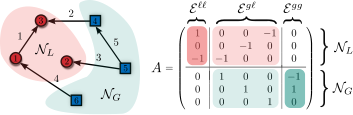
is the unique vector of branch-wise active power flows, satisfying Kirchhoff’s current law $P=Ap$. The branch flows $p$ of inherit the partitioning of the branches, and $A$ inherits the bus and branch partitions and may be written as the block matrix

Figure 1 illustrates these conventions on a simple network.

Since each element of $A$ is either $\pm 1$ or zero, we may write $A$ as the difference two binary matrices $A=A(+)-A(-)$, which have the analogous partitionings

The matrix $A(+)$ indexes the buses at the sending end of each branch, while $A(-)$ indexes the corresponding receiving end buses.²² 2 Due to our branch orientation conventions, $A_{L}^{g\ell}(+)=A_{G}^{g\ell}(-)=\mathbbold{0}$. We also will use an “unoriented” version $|A|$ of the incidence matrix $A$, with all non-zero elements set to +1:

In this section we cover in detail the solution of the canonical two-bus power system model [2, Chapter 2]. The insights we gain from a detailed analysis of this problem will help us properly understand our main results, as we will obtain analogous results for networks by analyzing the FPPF. The material here is known, but our treatment is quite non-standard.

The two-bus system depicted in Figure 2 consists of a single PV bus connected to a single PQ bus. The transmission line has a susceptance $-b<0$ and the PQ bus demands a constant complex power $-(P_{L}+\boldsymbol{\mathrm{j}}Q_{L})$.

In this case, the power flow equations (3a)–(3b) reduce to

where subscripts denote generation and load, respectively, and $\eta$ is the difference in phase angles between the two buses. We assume without loss of generality that $P_{G}=-P_{L}$; this is a necessary condition for (8) to be solvable (Section III-A). The incidence matrix is given by $A=\begin{pmatrix}-1&1\end{pmatrix}^{\sf T}$, and since the network is radial, Kirchhoff’s current law $\begin{pmatrix}P_{L}&P_{G}\end{pmatrix}^{\sf T}=Ap$ has the unique solution $p=P_{G}$ for the branch active power flow $p$. It follows that $p$ satisfies

We restrict our attention to (8c) and (9), which have unknowns $V_{L}$ and $\eta$. Note that under open-circuit conditions, where $P_{G}=P_{L}=Q_{L}=0$, inspection yields that the unique open-circuit solution $(\eta^{*},V_{L}^{*})\in[-\frac{\pi}{2},\frac{\pi}{2}]\times\mathbb{R}_{>0}$ to (8c)–(9) is $V_{L}^{*}=V_{G}$ and $\eta^{*}=0$. The first step in solving (8c)–(9) is to eliminate $\eta$ by squaring both sides of both equations, adding, and using $\sin^{2}(\eta)+\cos^{2}(\eta)=1$ to arrive at the quartic equation

or equivalently

Now introduce the change of variables $v=V_{L}/V_{L}^{*}$, to the scaled voltage variable $v>0$. Inserting this into (10), collecting terms, and dividing through by constants, one obtains

where we have introduced the dimensionless active and reactive power variables $\Gamma,\Delta\in\mathbb{R}$ defined by³³ 3 While the sign of $\Gamma$ ends up being unimportant, $\Delta$ has been defined such that $\Delta>0$ corresponds to an inductively loaded network.

The nondimensionalized equation (11) is quadratic in $v^{2}$, with solutions

Both solutions take nonnegative real values if and only if

in which case the solutions

satisfy $v_{-}\in{[0,\frac{1}{\sqrt{2}})}$ and $v_{+}\in{(\frac{1}{2},1]}$, with ordering $v_{-}<v_{+}$. Under condition (14) then, it follows that (11) possesses a unique solution $v=v_{+}$ in the high-voltage set $\{v\in\mathbb{R}\;|\;v_{+}\leq v\leq 1\}$, and in this case the solution lives at the lower boundary of this set. This situation is depicted in Figure 3(a).

Having determined the load voltage, we can determine the phase angle difference $\eta$ by rearranging (9) to read as

Solutions are given by $\eta_{\pm}=\mathrm{sign}(p)\,\gamma_{\pm}$, where

These solutions satisfy $\gamma_{-}\in{[0,\frac{\pi}{4})}$ and $\gamma_{+}\in{[0,\frac{\pi}{2})}$, with the ordering $\gamma_{-}<\gamma_{+}$. In particular then, (9) possess a unique solution $\eta=\gamma_{-}$ in the small angle deviation set $\{\eta\in[-\frac{\pi}{2},\frac{\pi}{2}]\;|\;|\eta|\leq\gamma_{-}\}$, and in this case the solution lives on the boundary of this set. This situation is depicted in Figure 3(b). A weak version of these results is stated formally now.

The dimensionless and loading margins $\Gamma$ and $\Delta$ in (12) quantify the stress the network experiences under active and reactive loading, respectively. The numerator of each loading margin is the power demand, while the denominator of each quantifies the “stiffness” of the transmission network, in units of power. Roughly speaking then, the solvability condition (14) requires that the network should be strong enough to handle the power transfer demands placed upon it. When (14) holds, we are guaranteed the existence of exactly one solution with a load voltage no lower than $v_{+}$ and a phase angle difference no larger than $\gamma_{-}$. The main result of this paper is a generalization of Proposition III.1 to large networks. Moreover, as visible from Figure 3(a), there is a medium-voltage region in voltage-space $\{v\in\mathbb{R}\;|\;v_{-}<v<v_{+}\}$ that is devoid of solutions.

Assuming the block $B_{LL}$ in (2) is negative definite, we define the open-circuit load voltages $V_{L}^{*}\in\mathbb{R}^{n}_{>0}$ by

One may verify that $(\theta,V_{L})=(\mathbbold{0}_{n+m},V_{L}^{*})$ is a solution of (3a)–(3b) with strictly positive voltage magnitudes when $P=\mathbbold{0}_{n+m}$ and $Q_{L}=\mathbbold{0}_{n}$. Using these open-circuit voltages, we define the scaled voltage variables $v=[V_{L}^{*}]^{-1}V_{L}$ and define the $|\mathcal{E}|\times|\mathcal{E}|$ branch stiffness matrix $\mathsf{D}$ as the diagonal matrix⁴⁴ 4 With a slight abuse of notation, in (17) we also use $V_{i}^{*}$ or $V_{j}^{*}$ to denote any fixed PV bus voltage.

The branch stiffness matrix quantifies the strength of the transmission lines. Finally, using $B_{LL}$ and $V_{L}^{*}$ we define the $n\times n$ negative definite nodal stiffness matrix⁵⁵ 5 For a vector $x\in\mathbb{R}^{n}$, $[x]=\mathrm{diag}(x)$ is the associated diagonal matrix, $\boldsymbol{\sin}(x)=(\sin(x_{1}),\ldots,\sin(x_{n}))^{\sf T}$, and if $x$ is nonnegative, $\sqrt{x}=(\sqrt{x_{1}},\ldots,\sqrt{x_{n}})^{\sf T}$. The vector $\mathbbold{1}_{n}$ is the vector of all ones of dimension $n$.

The nodal stiffness matrix quantifies the strength of the transmission network between PQ buses. The stiffness matrices (18) and (19) directly generalize the denominators in (12).

To compress our notation, define the function $h:\mathbb{R}^{n}_{>0}\rightarrow\mathbb{R}^{|\mathcal{E}|}$ component-wise for any edge $e\sim(i,j)\in\mathcal{E}$ by

In vector form, $h(v)\in\mathbb{R}^{|\mathcal{E}|}$ inherits the branch partitioning

of the branches. The following result is [1, Corollary 3.7].

In other words, for radial networks the model (21)–(23) is equivalent to the model (3a)–(3b); see [1, Theorem 5.5] for the more general meshed case.

We first restrict ourselves to networks where PQ buses are not connected to one another; two example networks are shown in Figure 4. We allow for PQ buses to have multiple PV bus neighbors, as in Figure 4(a), and denote by PV ​​$(i)\subset\mathcal{N}_{G}$ the set of PV buses connected to the $i$th PQ bus:

There are no restrictions on the connections between PV buses, other than that the network be radial.

Under this assumption, $\mathcal{E}^{\ell\ell}=\emptyset$, and the final two terms in the FPPF (21) are discarded. In this case, the grounded susceptance matrix $B_{LL}$ in (2) is a diagonal matrix, and hence so is the nodal stiffness matrix $\mathsf{S}$ in (19), with strictly negative diagonal elements

where $B_{ii}=-\sum_{j\in\textsf{PV}(i)}\nolimits B_{ij}+b_{\mathrm{shunt},i}$. Therefore, $\mathsf{S}_{ii}$ measures how strongly PQ bus $i\in\mathcal{N}_{L}$ is connected to the neighboring generator buses $\textsf{PV}(i)$.

The statement of Theorem V.1 can feel intimidating, so we now spend some time walking the reader through it. The branch and nodal stiffness matrices $\mathsf{D}$ and $\mathsf{S}$ quantify the strength of the grid, in units of power. In the case considered here, $\mathsf{S}$ is diagonal, and $\Delta_{i}=Q_{i}/\mathsf{S}_{ii}$ is interpreted as the stress experienced by PQ bus $i\in\mathcal{N}_{L}$ due to reactive loading. Similarly, the ratio $\Gamma_{ji}=|p_{ji}|/\mathsf{D}_{ji}$ is the stress experienced by branch $(j,i)$ due to active power flow. Therefore $\Gamma_{i}$ in (24b) identifies the most stressed branch incident to PQ bus $i$. The quantities (24a)–(24c) generalize the two-bus definitions (12).

The conditions (25) are “low stress” conditions; if the stress is not too great, the network has a high-voltage solution. Roughly speaking, (25a) is a voltage stability condition for PQ buses, and limits the maximum downward pressure on PQ bus voltage magnitudes; this is a generalization of the two-bus condition (14), and the set for a particular bus $i$ is depicted in Figure 5. Analogously, (25b) is an angle stability condition for PV buses, which limits the power flowing between generators. No such condition appeared for the two-bus case, as the two-bus case does not have multiple PV buses. Together, the conditions (25) implicitly define a set of feasible power injections in the space of power variables. The “bus-by-bus” nature of the condition (25a) is not an accident. Indeed, the key to the proof is that for this class of networks, the FPPF decouples into $n$ independent scalar fixed-point equations, each of which can be analyzed independently.

The quantities $v_{i,+}$, $\gamma_{i}$, and $\gamma_{ij}$ give us extremely specific information on where this unique solution is in voltage and angle space. Every normalized PQ bus voltage $v_{i}=V_{i}/V_{i}^{*}$ is guaranteed to be above $v_{i,+}$, while the phase angle difference $|\eta_{ji}|$ between PQ bus $i\in\mathcal{N}_{L}$ to any neighboring PV bus $j\in\mathcal{N}_{G}$ is guaranteed to be less than $\gamma_{i}<\frac{\pi}{4}$. Similarly, $\gamma_{ij}<\frac{\pi}{2}$ bounds the power angles between connected PV buses $i,j\in\mathcal{N}_{G}$. Note that while angles between PV buses may reach as high as 90^∘, angles between PV and PQ buses are always less than 45^∘. The expression (27a) shows precisely how active and reactive power injections (quantified through $\Delta_{i}$ and $\Gamma_{i}$) influence voltage magnitudes. For example, (27a) could be used to generate estimates for PV and PQ curves.

Graphically, the results of Theorem V.1 are shown in Figure 6, where we plot the space of PQ bus voltage magnitudes for the network in Figure 4(b). Voltage-space is partitioned into three useful sets (i) a blue high-voltage set where the unique solution is found (ii) a red low-voltage set where undesirable solutions may or may not exist, and (iii) a grey medium-voltage and extra-high voltage set, which is devoid of solutions. The width of the grey medium-voltage set characterizes the “stability margin” of the system. In fact, a calculation using (27) shows that

Therefore, the margin with which the condition (25a) is satisfied is directly related to the proximity between the high-voltage solution and any low-voltage solution. In any of the described cases where the conditions (25) are also necessary, all solutions depicted in Figure 6 are located at the “corners” of their respective boxes, nearest the centre of the figure.

References

- [1] J. W. Simpson-Porco, “A theory of solvability for lossless power flow equations – Part I: Fixed-point power flow,” IEEE Transactions on Control of Network Systems, 2017.
- [2] T. Van Cutsem and C. Vournas, Voltage Stability of Electric Power Systems. Springer, 1998.
- [3] F. Dörfler, M. Chertkov, and F. Bullo, “Synchronization in complex oscillator networks and smart grids,” Proceedings of the National Academy of Sciences, vol. 110, no. 6, pp. 2005–2010, 2013.
- [4] J. W. Simpson-Porco, F. Dörfler, and F. Bullo, “Voltage collapse in complex power grids,” Nature Communications, vol. 7, no. 10790, 2016.
- [5] E. H. Spanier, Algebraic Topology. Springer, 1994.
- [6] W. Rudin, Principles of Mathematical Analysis, 3rd ed., ser. International Series in Pure and Applied Mathematics. McGraw-Hill, 1976.
- [7] A. J. Korsak, “On the question of uniqueness of stable load-flow solutions,” IEEE Transactions on Power Apparatus and Systems, vol. 91, no. 3, pp. 1093–1100, 1972.
- [8] C. J. Tavora and O. J. M. Smith, “Equilibrium analysis of power systems,” IEEE Transactions on Power Apparatus and Systems, vol. 91, no. 3, pp. 1131–1137, 1972.
- [9] A. Araposthatis, S. Sastry, and P. Varaiya, “Analysis of power-flow equation,” International Journal of Electrical Power & Energy Systems, vol. 3, no. 3, pp. 115–126, 1981.
- [10] A. Arapostathis and P. Varaiya, “Behaviour of three-node power networks,” International Journal of Electrical Power & Energy Systems, vol. 5, no. 1, pp. 22 – 30, 1983.
- [11] F. D. Galiana, “Power-voltage limitations imposed by the network structure of a power system,” in IEEE Conference on Power Industry Computer Applications (PICA), 1975, pp. 356–363.
- [12] J. Jarjis and F. D. Galiana, “Quantitative analysis of steady state stability in power networks,” IEEE Transactions on Power Apparatus and Systems, vol. 100, no. 1, pp. 318–326, 1981.
- [13] F. D. Galiana, “Analytical investigation of the power flow equations,” in American Control Conference, San Francisco, CA, USA, Jun. 1983, pp. 411–415.
- [14] Y. V. Makarov, D. J. Hill, and I. A. Hiskens, “Properties of quadratic equations and their application to power system analysis,” Electrical Power and Energy Systems, vol. 22, no. 5, pp. 313–323, 2000.
- [15] I. A. Hiskens and R. J. Davy, “Exploring the power flow solution space boundary,” IEEE Transactions on Power Systems, vol. 16, no. 3, pp. 389–395, 2001.
- [16] Y. V. Makarov, Z.-Y. Dong, and D. J. Hill, “On convexity of power flow feasibility boundary,” IEEE Transactions on Power Systems, vol. 23, no. 2, pp. 811–813, 2008.
- [17] Y. V. Makarov, B. Vyakaranam, D. Wu, B. Lee, Z. Hou, S. T. Elbert, and Z. H. Huang, “On the configuration of the us western interconnection voltage stability boundary,” in IEEE Transmission & Distribution Conference and Exposition, April 2014, pp. 1–5.
- [18] J. Baillieul and C. I. Byrnes, “Geometric critical point analysis of lossless power system models,” IEEE Transactions on Circuits and Systems, vol. 29, no. 11, pp. 724–737, 1982.
- [19] B. K. Johnson, “Extraneous and false load flow solutions,” IEEE Transactions on Power Apparatus and Systems, vol. 96, no. 2, pp. 524–534, 1977.
- [20] A. Klos and J. Wojcicka, “Physical aspects of the nonuniqueness of load flow solutions,” International Journal of Electrical Power & Energy Systems, vol. 13, no. 5, pp. 268–276, 1991.
- [21] D. K. Molzahn, D. Mehta, and M. Niemerg, “Towards topologically-based upper bounds on the number of power flow solutions,” in American Control Conference, Boston, MA, USA, Jul. 2016, pp. 5927–5932.
- [22] F. F. Wu, “Theoretical study of the convergence of the fast decoupled load flow,” IEEE Transactions on Power Apparatus and Systems, vol. 96, no. 1, pp. 268–275, 1977.
- [23] F. F. Wu and S. Kumagai, Limits on Power Injections for Power Flow Equations to Have Secure Solutions. Electronics Research Laboratory, College of Engineering, University of California, 1980.
- [24] ——, “Steady-state security regions of power systems,” IEEE Transactions on Circuits and Systems, vol. 29, no. 11, pp. 703–711, 1982.
- [25] J. Thorp, D. Schulz, and M. Ilić-Spong, “Reactive power-voltage problem: conditions for the existence of solution and localized disturbance propagation,” International Journal of Electrical Power & Energy Systems, vol. 8, no. 2, pp. 66–74, 1986.
- [26] M. Ilić, “Network theoretic conditions for existence and uniqueness of steady state solutions to electric power circuits,” in IEEE International Symposium on Circuits and Systems, San Diego, CA, USA, May 1992, pp. 2821–2828.
- [27] H. Chiang and M. Baran, “On the existence and uniqueness of load flow solution for radial distribution power networks,” IEEE Transactions on Circuits and Systems, vol. 37, no. 3, pp. 410–416, 1990.
- [28] S. Grijalva and P. W. Sauer, “A necessary condition for power flow Jacobian singularity based on branch complex flows,” IEEE Transactions on Circuits and Systems I: Fundamental Theory and Applications, vol. 52, no. 7, pp. 1406–1413, 2005.
- [29] S. Grijalva, “Individual branch and path necessary conditions for saddle-node bifurcation voltage collapse,” IEEE Transactions on Power Systems, vol. 27, no. 1, pp. 12–19, 2012.
- [30] B. C. Lesieutre, P. W. Sauer, and M. A. Pai, “Existence of solutions for the network/load equations in power systems,” IEEE Transactions on Circuits and Systems I: Fundamental Theory and Applications, vol. 46, no. 8, pp. 1003–1011, 1999.
- [31] W. Dib, A. E. Barabanov, R. Ortega, and F. Lamnabhi-Lagarrigue, “An explicit solution of the power balance equations of structure preserving power system models,” IEEE Transactions on Power Systems, vol. 24, no. 2, pp. 759–765, 2009.
- [32] F. Dörfler and F. Bullo, “Novel insights into lossless AC and DC power flow,” in IEEE Power & Energy Society General Meeting, Vancouver, BC, Canada, Jul. 2013.
- [33] N. Ainsworth and S. Grijalva, “A structure-preserving model and sufficient condition for frequency synchronization of lossless droop inverter-based ac networks,” IEEE Transactions on Power Systems, vol. 28, no. 4, pp. 4310–4319, Nov 2013.
- [34] N. Barabanov, R. Ortega, R. G. nó, and B. Polyak, “On existence and stability of equilibria of linear time-invariant systems with constant power loads,” IEEE Transactions on Circuits and Systems I: Regular Papers, vol. 63, no. 1, pp. 114–121, 2016.
- [35] S. Bolognani and S. Zampieri, “On the existence and linear approximation of the power flow solution in power distribution networks,” IEEE Transactions on Power Systems, vol. 31, no. 1, pp. 163–172, 2016.
- [36] S. Yu, H. D. Nguyen, and K. S. Turitsyn, “Simple certificate of solvability of power flow equations for distribution systems,” in IEEE Power & Energy Society General Meeting, Denver, CO, USA, Jul. 2015, pp. 1–5.
- [37] Z. Wang, B. Cui, and J. Wang, “A necessary condition for power flow insolvability in power distribution systems with distributed generators,” IEEE Transactions on Power Systems, 2016, to Appear.
- [38] C. Wang, A. Bernstein, J. Y. L. Boudec, and M. Paolone, “Explicit conditions on existence and uniqueness of load-flow solutions in distribution networks,” IEEE Transactions on Smart Grid, 2016, to Appear.
- [39] S. H. Low, “Convex relaxation of optimal power flow, part i: Formulations and equivalence,” IEEE Transactions on Control of Network Systems, vol. 1, no. 1, pp. 15–27, 2014.
- [40] ——, “Convex relaxation of optimal power flow, part ii: Exactness,” IEEE Transactions on Control of Network Systems, vol. 1, no. 2, pp. 1–13, 2014.
- [41] K. Dvijotham, S. Low, and M. Chertkov, “Convexity of energy-like functions: Theoretical results and applications to power system operations,” ArXiv, 2015.
- [42] K. Dvijotham, S. Low, and M. Chertkov, “Solving the power flow equations: A monotone operator approach,” Arxiv, vol. abs/1506.08472, 2015.
- [43] T. T. Lie and R. A. Schlueter, “Strong local observability and controllability of power systems,” in IEEE International Symposium on Circuits and Systems, Jun 1991, pp. 970–973.
- [44] M. K. Pal, “Voltage stability: analysis needs, modelling requirement, and modelling adequacy,” Generation, Transmission and Distribution, IEE Proceedings C, vol. 140, no. 4, pp. 279–286, 1993.
- [45] C. A. Cañizares, Ed., Voltage Stability Assessment: Concepts, Practices and Tools. IEEE-PES Power System Stability Subcommittee, Aug. 2002, Tech. Rep. PES-TR9.
- [46] C. A. Cañizares, “On bifurcations, voltage collapse and load modeling,” IEEE Transactions on Power Systems, vol. 10, no. 1, pp. 512–522, 1995.
- [47] R. Delabays, T. Coletta, and P. Jacquod, “Multistability of phase-locking in equal-frequency kuramoto models on planar graphs,” Journal of Mathematical Physics, vol. 58, no. 3, p. 032703, 2017.
- [48] D. J. Hill and G. Chen, “Power systems as dynamic networks,” in IEEE Int. Symposium on Circuits and Systems, Kos, Greece, May 2006, pp. 722–725.
- [49] P. Hines, E. Cotilla-Sanchez, and S. Blumsack, “Do topological models provide good information about electricity infrastructure vulnerability?” Chaos, vol. 20, p. 033122, 2010.
- [50] F. Dörfler and F. Bullo, “Exploring synchronization in complex oscillator networks,” in IEEE Conf. on Decision and Control, Maui, HI, USA, Dec. 2012, pp. 7157–7170.
- [51] P.-A. Löf, D. J. Hill, S. Arnborg, and G. Andersson, “On the analysis of long-term voltage stability,” International Journal of Electrical Power & Energy Systems, vol. 15, no. 4, pp. 229–237, 1993.
Appendix A Technical Lemmas
Lemma A.1
The matrix
is row-stochastic; that is, and .
Proof of Lemma A.1: First, note that since is a nonsingular -matrix, has nonpositive elements, and hence from (7) and (18) so does the product . We compute using (19) that
Since the susceptance matrix and the incidence matrix are related by , one may use the partitioning of the incidence matrix (5) to show that