跳到论文正文
W Papers独立论文阅读器 arXiv:1701.02044 论文正文 计算阅读时间 · 0%
引用这篇论文根据当前论文元数据生成,正式投稿前建议核对。


License: arXiv.org perpetual non-exclusive license
arXiv:1701.02044v1 [cs.IT] 09 Jan 2017

Macro diversity in Cellular Networks with Random Blockages

Abhishek K. Gupta    Jeffrey G. Andrews    Robert W. Heath    Jr ††thanks: A. K. Gupta (g.kr.abhishek@utexas.edu), J. G. Andrews (jandrews@ece.utexas.edu) and R. W. Heath Jr. (rheath@utexas.edu) are with Wireless Networking and Communication Group, The University of Texas at Austin, Austin, TX 78712 USA.††thanks: This work is supported in part by the National Science Foundation under Grant 1514275 and AT&T Laboratories.
Abstract

Blocking objects (blockages) between a transmitter and receiver cause wireless communication links to transition from line-of-sight (LOS) to non-line-of-sight (NLOS) propagation, which can greatly reduce the received power, particularly at higher frequencies such as millimeter wave (mmWave). We consider a cellular network in which a mobile user attempts to connect to two or more base stations (BSs) simultaneously, to increase the probability of at least one LOS link, which is a form of macrodiversity. We develop a framework for determining the LOS probability as a function of the number of BSs, when taking into account the correlation between blockages: for example, a single blockage close to the device – including the user’s own body – could block multiple BSs. We consider the impact of the size of blocking objects on the system reliability probability and show that macrodiversity gains are higher when the blocking objects are small. We also show that the BS density must scale as the square of the blockage density to maintain a given level of reliability.

I Introduction

Blocking objects – blockages – in the form of buildings, foliage, and people, can severely impact the performance of cellular networks by reducing the signal strength and thus SNR. Blocking’s effect is more severe at higher frequencies including mmWave, due to higher penetration losses and reduced diffraction [1, 2]. Therefore, LOS connections are highly desirable particularly for mmWave. In addition, a user can block the otherwise LOS signals due to its own body [3, 4], hurting the overall reliability of the communication links. To overcome blockage effects, macrodiversity can be leveraged whereby a user is connected to multiple BSs simultaneously, which clearly increases the chance for a LOS connection [5, 6]. The presence of large blockages results in correlation in the probability of NLOS propagation among BSs in the same general direction from the user, since the same object could block several LOS paths. The objective of this paper is to study the impact of blockages on the gains of macrodiversity including a realistic correlation model.

I-A Related Work

There are some approaches to handle the blockage problem and increase link reliability in cellular systems, in particular for mmWave frequencies. For example, using reflections from walls and other surfaces to steer around obstacles [7] or switching the beam from a LOS link to a NLOS link [8] can reduce impact of blockages. However, this reduces received power vs a LOS link. Another approach is to maintain link connectivity by use of relays and routing algorithms [9, 10]. However, this leads to other issues such as high latency and non-tractability, due to its complex algorithms and scheduling schemes. The third approach is to use macro diversity with multiple BSs [11, 6]. Macro diversity over shadowing fading was studied in [12, 13]. In [14], the performance of coordinated beamforming with dynamic BS clusters was studied. The work [15] studied the fundamental limits of cooperation for multicell cooperative networks with multiple receive antennas. In [6], the authors proposed a multi-BS architecture for 60 GHz WLAN in which a MAC layer access controller device is employed to enable each station to associate and cooperate with multiple BSs. In the proposed architecture, when one of wireless links is blocked, another BS can be selected to complete the remaining transmissions.

In the past, multiple approaches have been proposed to model and analyze blockages. Simulation based approaches to model blockages by using ray tracing [16] in a deterministic environment are numerically complex and not tractable. For tractability, blocking is often included in the shadowing model as an additional loss. This approach, however, is over-simplistic, for example, it does not include the impact of the length of a link over its blocking probability. Therefore, this approach may not be not suitable to analyze scenarios where blockages play a significant role in determining its performance which is the case with communication at higher frequencies including mmWave. In [17], a tractable approach using random Boolean model with linear segments [18, 19, 20] was proposed to model the random blockages in a cellular system. This model was extended in [21] to include rectangular blockages and in [4] to include circular blockages. In [1], this blockage model was incorporated in the analysis of cellular systems to study the impact of blockages on the system performance. It was shown in [1] that the link reliability and coverage probability depend on the blockage process as a function of the product of blockage density and average blockage length.

Recent analytical work [1, 4, 21] to analyze the impact of blockages in cellular systems assumes a single active link per user and does not include macro diversity. In [22], a stochastic geometry framework was used to derive macro diversity gain for mmWave system in presence of random blockages. It assumes, however, independence among blocking events of the different links. When simultaneous multiple links are considered, the larger blockages may decrease the diversity gains due to induced correlation in blocking of these links and the system performance may no longer remain just a function of the product of the blockage density and average blockage length. In [23], time correlation of blocking events caused by user mobility was studied for mmWave networks. Although the spatial and time correlation analysis are similar to each other (in the sense that the correlation among blocking of the link to the same user at two time stamps is similar to the correlation among blocking of the links to different BSs), there are some differences in the analysis, insights and the interpretation. Also, in [23], the transmitter to receiver distance is fixed, which may not be the case with random deployment of BSs and users. Characterizing the spatial correlation among blockages and studying its impact in a system with macro diversity is the main focus of this work.

I-B Contributions

In this paper, we evaluate the benefits of macro diversity for a mmWave cellular system in the presence of random blockages. The contributions of the paper are summarized as follows.

Analytical framework for dependent blocking. We present a framework to analyze the correlation of blockage events occurring in links from the user to multiple BSs in a cellular system with random blockages. For blockage processes with linear blockages, we compute the joint probability of these links being non-blocked. We consider a special case of blockages where blockages have uniformly distributed lengths and orientations and show that unlike the independent case, this probability depends on both the blockage density and maximum blockage length, not just the product of the two. We show that increasing the maximum blockage length while keeping the product constant increases the correlation among blockage events occurring in multiple links.

Gains from macro diversity. We use the proposed framework to evaluate gains in reliability obtained by the use of macro diversity. We consider a system where each user is connected to multiple BSs simultaneously. For this system, we compute the average probability of having at least one LOS BS out of all connected links (termed the reliability). We term the gain in reliability achieved by the use of multiple BSs connections macro diversity gain. We show that the required BS density to achieve a certain level of reliability can be decreased significantly by maintaining multiple BS links simultaneously. The correlation in blockage events decreases the macro diversity gain in comparison to the case where blocking is independent among links. We also show that to maintain same level of reliability, the BS density must scale as square of the blockage density.

Analyzing diversity gains in the presence of self-blocking. If the person using a mobile phone comes in between the serving BS and the mobile, its body can block signals from its own serving BSs which is known as self-blocking. This can be modeled by a cone at the user which blocks all BSs lying that cone. We assume that these multiple BSs are selected in a way to avoid self-blocking of all BSs at any time and derive the reliability for this case using stochastic geometry tools.

The rest of the paper is organized as follows. Section II explains the blockage and connectivity model. Section III considers a system with second order diversity and derive reliability for this system. Section IV extends the analysis to the general case of the n​thn\text{th} diversity order. Section V presents numerical results and explains the main insights of the paper. We conclude in Section VI.

II System Model

In this section, we describe three distinct aspects of the system model.

Network model. We consider a cellular network consisting of BSs whose locations are modeled as a homogeneous Poisson point process (PPP) with density λ\lambda and users with locations modeled as a stationary Point process (PP). We consider a typical user at the origin 𝐎\mathbf{O}. Let Λ={𝐱i,i∈𝐍}\Lambda=\{\mathbf{x}_{i},i\in\mathbf{N}\} denote the BS PPP where locations 𝐱i\mathbf{x}_{i} are ordered according to their distances RiR_{i} from the typical user.

Refer to caption
(a) center
Refer to caption
(b) center
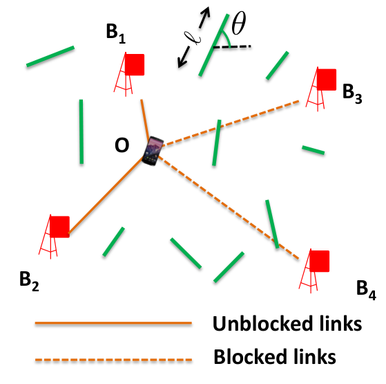
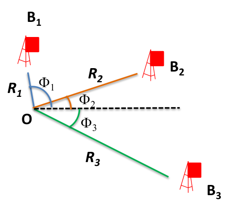
Fig. 1: System model: (a) An illustration showing a user at the origin in presence of blockages. Each blockage is modeled as linear segment of length ℓk\ell_{k} and orientation θk\theta_{k}. A link to any BS is said to be blocked or unreachable if a blockage falls on the link. (b) A cellular system with third order macro diversity (n=3n=3). The typical user at 𝐎\mathbf{O} has three active BSs it can associate with.

Modeling random blockages. To model the blockages present in the channel, we consider the line Boolean model Ψ\Psi similar to [17]. In this model, we assume that all the blockage elements are in the form of lines. In a real scenario, the blockages are polygon shaped. Since we are interested in their one dimensional intersections with the links, assuming their shapes as lines is a reasonable approximation. We also validate this model with real building data in Section V. The centers of these lines are modeled as a homogeneous PPP ψ\psi of density μ\mu. The lengths ℓk\ell_{k} of the blockage lines are independent identically distributed (iid) random variables with distribution FL​(⋅)F_{L}(\cdot). The orientations θk\theta_{k} of the blockage lines are assumed to be iid random variables with distribution FΘ​(⋅)F_{\Theta}(\cdot). Let us define the average LOS radius of a blockage process as 1/β1/\beta where β=μ​2π​𝔼​[ℓ]\beta=\mu\frac{2}{\pi}\mathbb{E}[\ell] [21]. The analysis performed in this paper can be in principle extended to Boolean models with other shapes such as rectangles or circles [21, 24], but it is left for future work. In this paper, we will also consider a special case of the above blockage process where ℓ\ell and θ\theta are uniformly distributed i.e. ℓ∼U⁡(0,Lmax),θ∼U⁡(0,π)\ell\sim U(0,L_{\mathrm{max}}),\theta\sim U(0,\pi) which is termed a uniform blockage process.

Connectivity model. We assume that all the users are simultaneously connected to the nn closest BSs (see Fig. 1(a)) where nn is the macro diversity order. We assume that a user will be able to quickly establish communication links with any of the nn BSs connected to it, using a well designed initial access process. Recall that the link to a BS can be LOS if there are no blockages intersecting the link between the BS and the user, otherwise the link is said to be in NLOS. Let 𝒜i\mathcal{A}_{i} denote the event that the i​thi\text{th} BS is LOS. At any point in time, the user will establish a communication link with the closest LOS BS, termed the associated BS out of these nn connected BSs. If all nn of the closest BSs are blocked, we say that the user is fully blocked.

We define the reliability pRp_{\mathrm{R}} as the probability that at least one connected BS out of the nn connected BSs is LOS to a typical user and is given as

pR\displaystyle p_{\mathrm{R}} =ℙ⁡[⋃i=1n𝒜i].\displaystyle=\mathbb{P}\left[\bigcup_{i=1}^{n}\mathcal{A}_{i}\right]. (1)

The reliability is useful from a system point of view. For example, a cellular operator may be interested in the question that if each user can use n​thn\text{th} order macro diversity, what the required BS density should be to achieve certain level of reliability.

TABLE I: Summary of Notation
Notation Description
Λ,λ\Lambda,\lambda The PPP modeling the BS locations, its density.
Ψ,ψ,μ\Psi,\psi,\mu The Boolean model for the blockage locations, the PPP modeling the centers of blockages and its density.
ℓk,θk\ell_{k},\theta_{k} The length and orientation of the k​thk\text{th} blockage.
FL​(),FΘ​()F_{L}(),F_{\Theta}() The distribution of blockage lengths ℓ\ell and orientations θ\theta. FL​(ℒ)F_{L}(\mathcal{L}) denotes the probability that ℓ∈ℒ\ell\in\mathcal{L}.
Ψ⁡(ℓ,θ)\Psi(\ell,\theta) The derived blockage process from Ψ\Psi consisting of blockages having length between ℓ\ell and ℓ+d​ℓ\ell+\mathrm{d}\ell and orientation between θ\theta and θ+d​θ\theta+\mathrm{d}\theta.
β,Lm\beta,L_{m} A parameter for the blockage process defined as μ​𝔼​[ℓ]​2π\mu\mathbb{E}\left[\ell\right]\frac{2}{\pi}, the maximum blockage length.
𝐁j,Ri,𝐙j\mathbf{B}_{j},R_{i},\mathbf{Z}_{j} The j​thj\text{th} closest BS from the user at the origin, the distance of this BS from the user, the link between this BS and the origin.
nn The order of macro diversity i.e. the number of simultaneous connected BSs.
Φi\Phi_{i} The angle between 𝐙j\mathbf{Z}_{j} and 𝐙n\mathbf{Z}_{n}.
Φ\Phi The angle between 𝐙1\mathbf{Z}_{1} and 𝐙2\mathbf{Z}_{2} for special case of second order diversity.
𝒜j\mathcal{A}_{j} The event that the j​thj\text{th} link is LOS.
pRp_{\mathrm{R}} The probability of reliability.
𝒫i\mathcal{P}_{i} The parallelogram constructed on the i​thi\text{th} link as shown in Fig. 2.
γ\gamma A parameter defined to be equal to β2​λ​π.\frac{\beta}{2\sqrt{\lambda\pi}}.
ω\omega The blocking cone created by the body of the user.

III Reliability Analysis for Second Order macro diversity

We will now compute the reliability for the system model described in the last section. To simplify, we will first consider a system of second order macro diversity (n=2n=2) and we will then extend the analysis to the general nn case. In the n=2n=2 case, the typical user is connected with two BSs, 𝐁1\mathbf{B}_{1} and 𝐁2\mathbf{B}_{2} with link lengths equal to R1R_{1} and R2R_{2}. Let us denote the angle between the two links 𝐙1\mathbf{Z}_{1} and 𝐙2\mathbf{Z}_{2} as Φ\Phi. Without loss of generality, we assume that 𝐱2\mathbf{x}_{2} is at xx axis and Φ≥0\Phi\geq 0. The joint distribution of R1R_{1} and R2R_{2} is given as

f⁡(r1,r2)\displaystyle f(r_{1},r_{2}) =(2​π​λ)2​r1​r2​exp⁡(−λ​π​r22), if ​r1≤r2\displaystyle=(2\pi\lambda)^{2}r_{1}r_{2}\exp(-\lambda\pi r_{2}^{2}),\text{ if }r_{1}\leq r_{2} (2)

and Φ∼Uniform​(0,π)\Phi\sim\text{Uniform}(0,\pi).

Now, let us consider a derived Boolean model Ψ⁡(ℓ,θ)\Psi(\ell,\theta) consisting of the blockages in Ψ\Psi with lengths between ℓ\ell and ℓ+d​ℓ\ell+\mathrm{d}\ell and orientations between θ\theta and θ+d​θ\theta+\mathrm{d}\theta. Note that the process containing the centers of these blockages can be obtained by thinning the original PP ψ\psi. Therefore, centers of Ψ⁡(ℓ,θ)\Psi(\ell,\theta) form a PPP with intensity μ​FL​(d​ℓ)​FΘ​(d​θ)\mu F_{L}(\mathrm{d}\ell)F_{\Theta}(\mathrm{d}\theta). Given the two links 𝐙𝟏\mathbf{Z_{1}} and 𝐙𝟐\mathbf{Z_{2}}, let 𝒜1\mathcal{A}_{1} and 𝒜2\mathcal{A}_{2} respectively denote the events that these links are unblocked. The probability that at least one of the links is not blocked is given as

ℙ⁡[𝒜1∪𝒜2]=ℙ⁡[𝒜1]+ℙ⁡[𝒜2]−ℙ⁡[𝒜1∩𝒜2].\displaystyle\mathbb{P}\left[\mathcal{A}_{1}\cup\mathcal{A}_{2}\right]=\mathbb{P}\left[\mathcal{A}_{1}\right]+\mathbb{P}\left[\mathcal{A}_{2}\right]-\mathbb{P}\left[\mathcal{A}_{1}\cap\mathcal{A}_{2}\right]. (3)
Refer to caption
Fig. 2: Illustration showing the joint area of the two parallelograms 𝒫1\mathcal{P}_{1} and 𝒫2\mathcal{P}_{2}. The parallelogram 𝒫1\mathcal{P}_{1} (or 𝒫2\mathcal{P}_{2}) represents the region where centers of any blockage must not lie for the links 𝐙1\mathbf{Z}_{1} (or 𝐙2\mathbf{Z}_{2}) to be LOS. Subfigures (a), (b) and (c) show shapes for the region 𝒰\mathcal{U} common in both parallelograms dependent on the values of ℓ,θ,R1,R2\ell,\theta,R_{1},R_{2} and Φ\Phi. The conditions are mentioned in the subfigures where d1d_{1} and d2d_{2} are lengths of AC and BC. Fig. (d) The triangle 𝒯\mathcal{T} circumscribes the common region 𝒰\mathcal{U}.

The event that the link 𝐙1\mathbf{Z}_{1} is not blocked by a blockage in Ψ⁡(ℓ,θ)\Psi(\ell,\theta) is equivalent to the event that the centers of all blockages in this collection Ψ⁡(ℓ,θ)\Psi(\ell,\theta) lie outside the parallelogram 𝒫1\mathcal{P}_{1} shown in Fig. 2(a). The area of 𝒫1\mathcal{P}_{1} is given as

A1​(R1,ℓ,θ,Φ)\displaystyle A_{1}(R_{1},\ell,\theta,\Phi) =ℓ​R1​sin⁡(|θ−Φ|).\displaystyle=\ell R_{1}\sin(|\theta-\Phi|).

Hence, the probability of the event that the link 𝐙1\mathbf{Z}_{1} is not blocked by an blockage in Ψ⁡(ℓ,θ)\Psi(\ell,\theta) is given by void probability of a PPP and is equal to exp⁡(−μ​FL​(d​ℓ)​FΘ​(d​θ)​A1​(R1,ϕ,ℓ,θ))\exp\left(-\mu F_{L}(\mathrm{d}\ell)F_{\Theta}(\mathrm{d}\theta)A_{1}(R_{1},\phi,\ell,\theta)\right). Therefore, the probability of the event 𝒜1\mathcal{A}_{1} that the link 𝐙1\mathbf{Z}_{1} is not blocked is

ℙ⁡[𝒜1]\displaystyle\mathbb{P}\left[\mathcal{A}_{1}\right] =∏ℓ,θexp⁡(−μ​FL​(d​ℓ)​FΘ​(d​θ)​A1​(R1,ϕ,ℓ,θ))\displaystyle=\prod_{\ell,\theta}\exp(-\mu F_{L}(\mathrm{d}\ell)F_{\Theta}(\mathrm{d}\theta)A_{1}(R_{1},\phi,\ell,\theta))
=exp(−∫0∞∫0πμA1(R1,ϕ,ℓ,θ)FL(dℓ)FΘ(dθ)).\displaystyle=\exp\left(-\int_{0}^{\infty}\int_{0}^{\pi}\mu A_{1}(R_{1},\phi,\ell,\theta)F_{L}(\mathrm{d}\ell)F_{\Theta}(\mathrm{d}\theta)\right). (4)

Using the value of area A1A_{1} in (4), we get

ℙ⁡[𝒜1]\displaystyle\mathbb{P}\left[\mathcal{A}_{1}\right] =exp(−∫0∞∫0πμℓR1sin(|θ−Φ|)FL(dℓ)FΘ(dθ))\displaystyle=\exp\left(-\int_{0}^{\infty}\int_{0}^{\pi}\mu\ell R_{1}\sin(|\theta-\Phi|)F_{L}(\mathrm{d}\ell)F_{\Theta}(\mathrm{d}\theta)\right)
=exp⁡(−μ​𝔼​[ℓ]​R1​2π)=exp⁡(−β​R1).\displaystyle=\exp\left(-\mu\mathbb{E}\left[\ell\right]R_{1}\frac{2}{\pi}\right)=\exp(-\beta R_{1}). (5)

Similarly the probability of the event 𝒜2\mathcal{A}_{2} that the link 𝐙2\mathbf{Z}_{2} is not blocked is

ℙ⁡[𝒜2]\displaystyle\mathbb{P}\left[\mathcal{A}_{2}\right] =exp(−∫0∞∫0πμA2(R2,ϕ,ℓ,θ)FL(dℓ)FΘ(dθ))=exp(−βR2).\displaystyle=\exp\left(-\int_{0}^{\infty}\int_{0}^{\pi}\mu A_{2}(R_{2},\phi,\ell,\theta)F_{L}(\mathrm{d}\ell)F_{\Theta}(\mathrm{d}\theta)\right)=\exp(-\beta R_{2}). (6)

Now we will compute the joint probability ℙ⁡[𝒜1∩𝒜2]\mathbb{P}\left[\mathcal{A}_{1}\cap\mathcal{A}_{2}\right]. Similar to the previous case, the event that both links are not blocked by any blockage in Ψ⁡(ℓ,θ)\Psi(\ell,\theta) is equivalent to the event that centers of all blockages in the collection Ψ⁡(ℓ,θ)\Psi(\ell,\theta) lie outside the shaded region (which is the union of two parallelograms 𝒫1\mathcal{P}_{1} and 𝒫2\mathcal{P}_{2}) shown in Fig. 2. Let A⁡(R1,R2,ϕ,ℓ,θ)A(R_{1},R_{2},\phi,\ell,\theta) be the area of shaded region. The shape of the intersection (denoted by 𝒰\mathcal{U}) of the two parallelograms can be triangular or trapezoidal, dependent on the values of R1,R2,Φ,θ,ℓR_{1},R_{2},\Phi,\theta,\ell (See Fig. 2(a-c)). Let triangle 𝒯\mathcal{T} denote the triangle (Δ\DeltaABC) circumscribing 𝒰\mathcal{U}. The area of this triangle is

T=ℓ2​sin⁡(θ)​sin⁡(|θ−Φ|)2​sin⁡(Φ).\displaystyle T=\frac{\ell^{2}\sin(\theta)\sin(|\theta-\Phi|)}{2\sin(\Phi)}.

The trapezoidal shape occurs only when R1<ℓ1R_{1}<\ell_{1} or R2<ℓ2R_{2}<\ell_{2}. The area of 𝒯∖𝒰\mathcal{T}\setminus\mathcal{U} is given by (1−min⁡(R2ℓ1,R1ℓ2))2​T\left(1-\min\left(\frac{R_{2}}{\ell_{1}},\frac{R_{1}}{\ell_{2}}\right)\right)^{2}T. Therefore, the area of 𝒫1∪𝒫2\mathcal{P}_{1}\cup\mathcal{P}_{2} is

A⁡(R1,R2,Φ,ℓ,θ)=ℓ​R1​sin⁡(|θ−Φ|)+ℓ​R2​sin⁡(θ)\displaystyle A(R_{1},R_{2},\Phi,\ell,\theta)=\ell R_{1}\sin(|\theta-\Phi|)+\ell R_{2}\sin(\theta)
−1​(θ>ϕ)​ℓ2​sin⁡(θ)​sin⁡(θ−Φ)2​sin⁡(Φ)​[1−(1−min⁡(1,R1​sin⁡(Φ)ℓ​sin⁡(θ)​R2​sin⁡(Φ)ℓ​sin⁡(θ−Φ)))2].\displaystyle\ \ \ -1(\theta>\phi)\frac{\ell^{2}\sin(\theta)\sin(\theta-\Phi)}{2\sin(\Phi)}\left[1-\left(1-\min\left(1,\frac{R_{1}\sin(\Phi)}{\ell\sin(\theta)}\frac{R_{2}\sin(\Phi)}{\ell\sin(\theta-\Phi)}\right)\right)^{2}\right]. (7)

Hence, the probability that both of the links are not blocked by Ψ⁡(ℓ,θ)\Psi(\ell,\theta) is exp⁡(−μ​FL​(d​ℓ)​FΘ​(d​θ)CLOSE\exp\left(-\mu F_{L}(\mathrm{d}\ell)F_{\Theta}(\mathrm{d}\theta)\right. OPENA⁡(R1,R2,ϕ,ℓ,θ))\left.A(R_{1},R_{2},\phi,\ell,\theta)\right). Therefore, the probability that both links are not blocked is

ℙ⁡[𝒜1∩𝒜2]\displaystyle\mathbb{P}\left[\mathcal{A}_{1}\cap\mathcal{A}_{2}\right] =∏ℓ,θexp⁡(−μ​FL​(d​ℓ)​FΘ​(d​θ)​A​(R1,R2,ϕ,ℓ,θ))\displaystyle=\prod_{\ell,\theta}\exp(-\mu F_{L}(\mathrm{d}\ell)F_{\Theta}(\mathrm{d}\theta)A(R_{1},R_{2},\phi,\ell,\theta))
=exp(−∫0∞∫0πμA(R1,R2,ϕ,ℓ,θ)FL(dℓ)FΘ(dθ))\displaystyle=\exp\left(-\int_{0}^{\infty}\int_{0}^{\pi}\mu A(R_{1},R_{2},\phi,\ell,\theta)F_{L}(\mathrm{d}\ell)F_{\Theta}(\mathrm{d}\theta)\right) (8)

Let us define 𝒩⁡(R1,R2,Φ)\mathcal{N}(R_{1},R_{2},\Phi) as the mean shaded area averaged over blockage size and orientation distribution:

𝒩⁡(R1,R2,Φ)\displaystyle\mathcal{N}(R_{1},R_{2},\Phi) =∫0∞∫0πA⁡(R1,R2,ϕ,ℓ,θ)​FL​(𝑑ℓ)​FΘ​(𝑑θ).\displaystyle=\int_{0}^{\infty}\int_{0}^{\pi}A(R_{1},R_{2},\phi,\ell,\theta)F_{L}(\mathrm{d}\ell)F_{\Theta}(\mathrm{d}\theta). (9)

Then, ℙ⁡[𝒜1∩𝒜2]\mathbb{P}\left[\mathcal{A}_{1}\cap\mathcal{A}_{2}\right] is given by

ℙ⁡[𝒜∩𝒜2]=p⁡(R1,R2,Φ)\displaystyle\mathbb{P}\left[\mathcal{A}\cap\mathcal{A}_{2}\right]=p(R_{1},R_{2},\Phi) =exp⁡(−μ​𝒩​(R1,R2,Φ)).\displaystyle=\exp\left(-\mu\mathcal{N}(R_{1},R_{2},\Phi)\right). (10)

Therefore, using (3), the probability that at least one of the links is not blocked is equal to

ℙ⁡[𝒜1∪𝒜2]=exp⁡(−β​R1)+exp⁡(−β​R2)−exp⁡(−μ​𝒩​(R1,R2,Φ)).\displaystyle\mathbb{P}\left[\mathcal{A}_{1}\cup\mathcal{A}_{2}\right]=\exp(-\beta R_{1})+\exp(-\beta R_{2})-\exp\left(-\mu\mathcal{N}(R_{1},R_{2},\Phi)\right). (11)

Now, the reliability can be computed as

pR=𝔼R1,R2​[ℙ⁡[𝒜1∪𝒜2]]\displaystyle p_{\mathrm{R}}=\mathbb{E}_{R_{1},R_{2}}\left[\mathbb{P}\left[\mathcal{A}_{1}\cup\mathcal{A}_{2}\right]\right]
=1π​∫0∞∫0∞∫0π(exp⁡(−β​r1)+exp⁡(−β​r2)−exp⁡(−μ​𝒩​(r1,r2,ϕ)))​fR1,R2​(r1,r2)​𝑑ϕ​d​r1​d​r2\displaystyle=\frac{1}{\pi}\int_{0}^{\infty}\int_{0}^{\infty}\int_{0}^{\pi}\left(\exp(-\beta r_{1})+\exp(-\beta r_{2})-\exp\left(-\mu\mathcal{N}(r_{1},r_{2},\phi)\right)\right)f_{R_{1},R_{2}}(r_{1},r_{2})\mathrm{d}\phi\mathrm{d}r_{1}\mathrm{d}r_{2}
=(2​π​λ)2π​∫0∞∫0r2∫0π(exp⁡(−β​r1)+exp⁡(−β​r2)CLOSE\displaystyle=\frac{(2\pi\lambda)^{2}}{\pi}\int_{0}^{\infty}\int_{0}^{r_{2}}\int_{0}^{\pi}\left(\exp(-\beta r_{1})+\exp(-\beta r_{2})\right.
OPEN−exp⁡(−μ​𝒩​(r1,r2,ϕ)))​r1​r2​exp⁡(−λ​π​r22)​d​ϕ​d​r1​d​r2.\displaystyle\hskip 144.54pt\left.-\exp\left(-\mu\mathcal{N}(r_{1},r_{2},\phi)\right)\right)r_{1}r_{2}\exp(-\lambda\pi r_{2}^{2})\mathrm{d}\phi\mathrm{d}r_{1}\mathrm{d}r_{2}. (12)

Using the transformations x1=β​r1,x2=β​r2x_{1}=\beta r_{1},x_{2}=\beta r_{2},

pR=14​γ4​π​∫0∞∫0x2∫0π(e−x1+e−x2−e−μ​s​(x1β,x2β,ϕ))​x1​x2​e−x224​γ2​𝑑ϕ​d​x1​d​x2\displaystyle p_{\mathrm{R}}=\frac{1}{4\gamma^{4}\pi}\int_{0}^{\infty}\int_{0}^{x_{2}}\int_{0}^{\pi}\left(e^{-x_{1}}+e^{-x_{2}}-e^{-\mu s\left(\frac{x_{1}}{\beta},\frac{x_{2}}{\beta},\phi\right)}\right)x_{1}x_{2}e^{-\frac{x_{2}^{2}}{4\gamma^{2}}}\mathrm{d}\phi\mathrm{d}x_{1}\mathrm{d}x_{2} (13)

where

γ=β2​π​λ.\displaystyle\gamma=\frac{\beta}{2\sqrt{\pi\lambda}}. (14)

Here, γ\gamma equals half the ratio of average cell radius (1/π​λ1/\sqrt{\pi\lambda}) and average LOS radius (1/β1/\beta) and therefore, represents the relative blockage size with respect to the BS deployment. Solving the first two integrals in (13), we get the final expression for the reliability given in the following Theorem.

Theorem 1.

The reliability in a cellular network with second order macro diversity is

pR\displaystyle p_{\mathrm{R}} =2+γ2−γ⁡(5+2​γ2)​W​(γ)−\displaystyle=2+\gamma^{2}-\gamma(5+2\gamma^{2})W(\gamma)-
14​γ4​π​∫0π∫0∞x2​exp⁡(−x224​γ2)​∫0x2exp⁡(−μ​𝒩​(x1β,x2β,ϕ))​x1​d​x1​d​x2​𝑑ϕ\displaystyle\frac{1}{4\gamma^{4}\pi}\int_{0}^{\pi}\int_{0}^{\infty}x_{2}\exp\left(-\frac{x_{2}^{2}}{4\gamma^{2}}\right)\int_{0}^{x_{2}}\exp\left(-\mu\mathcal{N}\left(\frac{x_{1}}{\beta},\frac{x_{2}}{\beta},\phi\right)\right)x_{1}\mathrm{d}x_{1}\mathrm{d}x_{2}\mathrm{d}\phi (15)

where 𝒩⁡(r1,r2,ϕ)\mathcal{N}(r_{1},r_{2},\phi) is given in (9), and

W⁡(x)=π2​erfcx​(x)=π​exp⁡(x2)​Q​(2​x).\displaystyle W(x)=\frac{\sqrt{\pi}}{2}\mathrm{erfcx}(x)=\sqrt{\pi}\exp{(x^{2})}\mathrm{Q}\left(\sqrt{2}x\right). (16)

Before going further, we will give the following Lemma regarding the monotonicity of reliability with respect to blockage length’s distribution.

Lemma 1.

For all the blockage processes with the same parameter β\beta and scaled distribution Fc′​(d​ℓ)=FL​(d​ℓ/c)F^{\prime}_{c}(\mathrm{d}\ell)=F_{L}(\mathrm{d}\ell/c) of length, the quantity μ​𝒩​(R1,R2,Φ)\mu\mathcal{N}(R_{1},R_{2},\Phi), as defined in (9), monotonically decreases with increasing cc and so does the reliability.

Proof:

See Appendix A. ∎

Note that for the uniform blockage process with blockage length ℓ∼U⁡(0,Lmax)\ell\sim U(0,L_{\mathrm{max}}), scaling the distribution by cc, is equivalent to increasing the maximum length LmaxL_{\mathrm{max}} by cc. Therefore, one direct result of the Lemma 1 for the uniform blockage process is that the reliability decreases with increasing LmaxL_{\mathrm{max}}. This result is intuitive as fewer but more bulky blockages make the blocking probability of two links more correlated while small but more blockages result in independence between blocking of any two links.

The function 𝒩⁡(⋅,⋅,⋅)\mathcal{N}(\cdot,\cdot,\cdot) in Lemma 1 is dependent on the distribution of ℓ\ell and θ\theta. In general, this function is difficult to compute. In the next subsections, we will consider a few special cases to simplify the function 𝒩⁡(⋅,⋅,⋅)\mathcal{N}(\cdot,\cdot,\cdot) to get closed form expressions for the reliability.

III-A Reliability for Independent Blocking

In this subsection, we consider the independent blocking scenario where both links are blocked or not independently. Then, ℙ⁡[𝒜1∩𝒜2]\mathbb{P}\left[\mathcal{A}_{1}\cap\mathcal{A}_{2}\right] is equal to

ℙIND​[𝒜1∩𝒜2]=ℙ⁡[𝒜1]​ℙ​[𝒜2]=exp⁡(−β​R1−β​R2).\displaystyle\mathbb{P}_{\mathrm{IND}}\left[\mathcal{A}_{1}\cap\mathcal{A}_{2}\right]=\mathbb{P}\left[\mathcal{A}_{1}\right]\mathbb{P}\left[\mathcal{A}_{2}\right]=\exp(-\beta R_{1}-\beta R_{2}). (17)

Note that the area of 𝒫1∪𝒫2\mathcal{P}_{1}\cup\mathcal{P}_{2} is greater than the sum of the areas of the two parallelograms i.e.

A⁡(R1,R2,Φ,ℓ,θ)\displaystyle A(R_{1},R_{2},\Phi,\ell,\theta) ≤ℓ​R1​sin⁡(|θ−Φ|)+ℓ​R2​sin⁡(θ).\displaystyle\leq\ell R_{1}\sin(|\theta-\Phi|)+\ell R_{2}\sin(\theta).

Averaging with respect to ℓ\ell and θ\theta, we can upper bound mean shaded area as

𝒩⁡(R1,R2,Φ)\displaystyle\mathcal{N}(R_{1},R_{2},\Phi) ≤μ​𝔼​[ℓ]​2π​(R1+R2)\displaystyle\leq\mu\mathbb{E}\left[\ell\right]\frac{2}{\pi}(R_{1}+R_{2})
ℙ⁡[𝒜1∩𝒜2]\displaystyle\mathbb{P}\left[\mathcal{A}_{1}\cap\mathcal{A}_{2}\right] =exp⁡(−μ​𝒩​(R1,R2,Φ))≥exp⁡(−β​R1−β​R2)=ℙIND​[𝒜1∩𝒜2].\displaystyle=\exp(-\mu\mathcal{N}(R_{1},R_{2},\Phi))\geq\exp(-\beta R_{1}-\beta R_{2})=\mathbb{P}_{\mathrm{IND}}\left[\mathcal{A}_{1}\cap\mathcal{A}_{2}\right]. (18)

Therefore, the independent blocking case upper bounds the reliability in the dependent blocking scenario. Hence, we denote it by the notation pR¯\overline{p_{\mathrm{R}}}. We now provide the exact expression of the reliability for the independent blocking case in the following Theorem.

Theorem 2.

The reliability in a cellular network with second order diversity and independent blocking is

pR¯\displaystyle\overline{p_{\mathrm{R}}} =1γ​[γ3−W⁡(γ)​(2​γ4+5​γ2−1)+W⁡(2​γ)​(8​γ2−1)]\displaystyle=\frac{1}{\gamma}\left[\gamma^{3}-W(\gamma)(2\gamma^{4}+5\gamma^{2}-1)+W(2\gamma)(8\gamma^{2}-1)\right] (19)

where W⁡(⋅)W(\cdot) is given in (16).

Proof:

See Appendix B. ∎The above Theorem directly gives the following Corollary.

Corollary 1.

Given a certain target value of pR¯\overline{p_{\mathrm{R}}}, the required BS density with independent blocking is given by λ=β24​π​γs2\lambda=\frac{\beta^{2}}{4\pi\gamma_{s}^{2}} where γs\gamma_{s} is the solution of the following equation

γ3−W⁡(γ)​(2​γ4+5​γ2−1)+W⁡(2​γ)​(8​γ2−1)−γ​pR¯=0.\displaystyle\gamma^{3}-W(\gamma)(2\gamma^{4}+5\gamma^{2}-1)+W(2\gamma)(8\gamma^{2}-1)-\gamma\overline{p_{\mathrm{R}}}=0. (20)

Given pR¯\overline{p_{\mathrm{R}}}, (20) can be solved for γ\gamma using a numerical method.

III-B Reliability for Uniform Blockage Process

In this subsection, we will consider a uniform blockage process and provide bounds for the reliability. In a uniform blockage process, the length and orientation of blockages are uniformly distributed. For this case, the average LOS radius is given as β=μ​Lmax/π\beta=\mu L_{\mathrm{max}}/\pi where LmaxL_{\mathrm{max}} is the maximum length of blockages.

III-B1 Lower Bound I

Note that the area AA is the sum of A1A_{1} (the area of 𝒫1\mathcal{P}_{1}) and A2A_{2} (the area of 𝒫2\mathcal{P}_{2}) minus the area of the common region 𝒰\mathcal{U} (in shape of either a trapezoid or a triangle). We can lower bound this area AA by replacing the area of 𝒰\mathcal{U} by the area of its circumscribing triangle 𝒯\mathcal{T}. Note that for certain values of θ\theta and ℓ\ell, the area of 𝒯\mathcal{T} may become greater than the area of parallelogram 𝒫1\mathcal{P}_{1}. In this case, we can lower bound the area AA by just the area of parallelogram 𝒫2\mathcal{P}_{2}. Hence, we get the following lower bound for area AA:

A⁡(R1,R2,ϕ,ℓ,θ)\displaystyle A(R_{1},R_{2},\phi,\ell,\theta) ≥{A1+A2 for ​θ≤ϕA1+A2−Tfor ​π>θ>ϕ,sin⁡(θ)<2​R1​sin⁡(ϕ)/ℓA2for π>θ>ϕ,1≥sin(θ)>2R1sin(ϕ)/ℓ.\displaystyle\geq\begin{cases}A_{1}+A_{2}&\text{ for }\theta\leq\phi\\ A_{1}+A_{2}-T&\text{for }\pi>\theta>\phi,\sin(\theta)<{2R_{1}\sin(\phi)}/{\ell}\\ A_{2}&\text{for }\pi>\theta>\phi,1\geq\sin(\theta)>{2R_{1}\sin(\phi)}/{\ell}.\end{cases} (21)

Now, integrating (21) with respect to distribution of θ\theta and ℓ\ell gives the lower bound for 𝒩⁡(R1,R2,Φ)\mathcal{N}(R_{1},R_{2},\Phi) which is denoted by 𝒩¯¯​(R1,R2,Φ)\underline{\underline{\mathcal{N}}}(R_{1},R_{2},\Phi) and given as

𝒩⁡(R1,R2,Φ)≥𝒩¯¯​(R1,R2,Φ)=Lmaxπ​(R1+R2−R1​F​(R1Lmax,Φ))\displaystyle\mathcal{N}(R_{1},R_{2},\Phi)\geq\underline{\underline{\mathcal{N}}}(R_{1},R_{2},\Phi)=\frac{L_{\mathrm{max}}}{\pi}\left(R_{1}+R_{2}-R_{1}F\left(\frac{R_{1}}{L_{\mathrm{max}}},\Phi\right)\right)

where F⁡(a,Φ)=F(a,\Phi)=

{0<Φ≤π2{2​a≤112+a3​(2​a−3)​sin2⁡(Φ)+13​T1−23​T2+43​T3−23​T4+112​T62​a>1,2​a​sin⁡(Φ)≤112−a⁡(2​a+1)​sin2⁡(Φ)+13​T1−23​T2+23​T3+112​T6+T72​a​sin⁡(Φ)≥1112​a​(1+(π−Φ)​cot⁡(Φ))π2<Φ<π{2​a≤112+a3​(2​a−3)​sin2⁡(Φ)+13​T1−23​T2+23​T5+112​T62​a>1112​a​(1+(π−Φ)​cot⁡(Φ))\displaystyle\begin{cases}0<\Phi\leq\frac{\pi}{2}&\begin{cases}2a\leq 1&\frac{1}{2}+\frac{a}{3}(2a-3)\sin^{2}(\Phi)+\frac{1}{3}T_{1}-\frac{2}{3}T_{2}+\frac{4}{3}T_{3}-\frac{2}{3}T_{4}+\frac{1}{12}T_{6}\\ 2a>1,2a\sin(\Phi)\leq 1&\frac{1}{2}-a(2a+1)\sin^{2}(\Phi)+\frac{1}{3}T_{1}-\frac{2}{3}T_{2}+\frac{2}{3}T_{3}+\frac{1}{12}T_{6}+T_{7}\\ 2a\sin(\Phi)\geq 1&\frac{1}{12a}(1+(\pi-\Phi)\cot(\Phi))\end{cases}\\ \frac{\pi}{2}<\Phi<\pi&\begin{cases}2a\leq 1&\hskip 72.26999pt\frac{1}{2}+\frac{a}{3}(2a-3)\sin^{2}(\Phi)+\frac{1}{3}T_{1}-\frac{2}{3}T_{2}+\frac{2}{3}T_{5}+\frac{1}{12}T_{6}\\ 2a>1&\hskip 72.26999pt\frac{1}{12a}(1+(\pi-\Phi)\cot(\Phi))\end{cases}\end{cases}

with

T1\displaystyle T_{1} =cos⁡(Φ)​1−4​a2​sin2⁡(Φ)\displaystyle=\cos(\Phi)\sqrt{1-{4a^{2}\sin^{2}(\Phi)}} T2\displaystyle T_{2} =a2​sin2⁡(Φ)​cos⁡(Φ)​log⁡(1+1−4​a2​sin2⁡(Φ))\displaystyle=a^{2}\sin^{2}(\Phi)\cos(\Phi)\log\left(1+\sqrt{1-4a^{2}\sin^{2}(\Phi)}\right)
T3\displaystyle T_{3} =a2​sin2⁡(Φ)​cos⁡(Φ)​log⁡(2​a​sin⁡(Φ))\displaystyle=a^{2}\sin^{2}(\Phi)\cos(\Phi)\log(2a\sin(\Phi)) T4\displaystyle T_{4} =a2​sin2⁡(Φ)​cos⁡(Φ)​log⁡(2​a​(1+cos⁡(Φ)))\displaystyle=a^{2}\sin^{2}(\Phi)\cos(\Phi)\log(2a(1+\cos(\Phi)))
T5\displaystyle T_{5} =a2​sin2⁡(Φ)​cos⁡(Φ)​log⁡(2​a​(1−cos⁡(Φ)))\displaystyle=a^{2}\sin^{2}(\Phi)\cos(\Phi)\log(2a(1-\cos(\Phi))) T6\displaystyle T_{6} =1a​cot⁡(Φ)​sin−1⁡(2​a​sin⁡(Φ))\displaystyle=\frac{1}{a}\cot(\Phi)\sin^{-1}\left(2a\sin(\Phi)\right)
T7\displaystyle T_{7} =(π−2​Φ)3​a2​sin2⁡(Φ)​cos⁡(Φ).\displaystyle=\frac{(\pi-2\Phi)}{3}a^{2}\sin^{2}(\Phi)\cos(\Phi).

Note that F⁡(a,0)=1F(a,0)=1 and F⁡(a,π)=0F(a,\pi)=0.

It can be seen that the lower bound on the mean area 𝒩¯¯​(R1,R2,Φ)\underline{\underline{\mathcal{N}}}(R_{1},R_{2},\Phi) is dependent on both the blocking parameter β\beta and the maximum blockage length LmaxL_{\mathrm{max}}. The monotonicity of AA with respect to LmaxL_{\mathrm{max}} (as shown in Lemma 1) implies that for a constant β\beta, as LmaxL_{\mathrm{max}} increases (which means fewer but larger blockages), F⁡(a,Φ)F(a,\Phi) increases towards 12​(1+cos⁡(Φ))\frac{1}{2}(1+\cos(\Phi)). For small LmaxL_{\mathrm{max}}, (which means more but smaller blockages), F⁡(a,Φ)F(a,\Phi) decreases to 00 which corresponds to the independent case. For intermediate values of LmaxL_{\mathrm{max}}, F⁡(a,Φ)F(a,\Phi) will range between 00 and 12​(1+cos⁡(Φ))\frac{1}{2}(1+\cos(\Phi)).

Now, the lower bound on reliability can be obtained by using Theorem 1:

pR≥\displaystyle p_{\mathrm{R}}\geq pR¯¯=2+γ2−γ⁡(5+2​γ2)​W​(γ)\displaystyle\ \underline{\underline{p_{\mathrm{R}}}}=2+\gamma^{2}-\gamma(5+2\gamma^{2})W(\gamma)
−12​γ2​π∫0π∫0∞exp(−x1(1−F(x1/(βLmax),ϕ)))x1S(x1)dx1dϕ\displaystyle-\frac{1}{2\gamma^{2}\pi}\int_{0}^{\pi}\int_{0}^{\infty}\exp(-x_{1}(1-F(x_{1}/(\beta L_{\mathrm{max}}),\phi)))x_{1}S(x_{1})dx_{1}\mathrm{d}\phi

where S⁡(x)=exp⁡(γ2−(12​γ​x+γ)2)​[1−2​γ​W​(12​γ​x+γ)]S(x)=\exp\left(\gamma^{2}-\left(\frac{1}{2\gamma}x+\gamma\right)^{2}\right)\left[1-2\gamma W\left(\frac{1}{2\gamma}x+\gamma\right)\right].

III-B2 Asymptotic Lower Bound

We can bound the Area AA as follows:

A⁡(R1,R2,ϕ,ℓ,θ)\displaystyle A(R_{1},R_{2},\phi,\ell,\theta) ≥{A1+A2 for ​θ≤ϕA2for ​π>θ>ϕ.\displaystyle\geq\begin{cases}A_{1}+A_{2}&\text{ for }\theta\leq\phi\\ A_{2}&\text{for }\pi>\theta>\phi\end{cases}. (22)

Now, integrating (22) with respect to θ\theta and ℓ\ell gives the following lower bound (denoted by 𝒩¯\underline{\mathcal{N}}) for mean area 𝒩⁡(R1,R2,Φ)\mathcal{N}(R_{1},R_{2},\Phi):

𝒩⁡(R1,R2,Φ)≥𝒩¯​(R1,R2,Φ)=Lmaxπ​(R1+R2−R1​12​(1+cos⁡(Φ))).\displaystyle\mathcal{N}(R_{1},R_{2},\Phi)\geq\underline{\mathcal{N}}(R_{1},R_{2},\Phi)=\frac{L_{\mathrm{max}}}{\pi}\left(R_{1}+R_{2}-R_{1}\frac{1}{2}\left(1+\cos(\Phi)\right)\right). (23)

As discussed in the previous subsection, for a given β\beta, the lower bound becomes asymptotically tight as maximum blockage length Lmax→∞L_{\mathrm{max}}\rightarrow\infty. Now, using the lower bound in (23) and Theorem 1, a lower bound (denoted by pR¯\underline{p_{\mathrm{R}}}) on reliability probability can be obtained as follows (see Appendix C):

pR\displaystyle p_{\mathrm{R}} OPEN≥pR¯=1+γ2−γ⁡(5+2​γ2)​W​(γ)+4​γπ​∫0π/2(2+sin2⁡(ϕ))​W​((1+sin2⁡(ϕ))​γ))​𝑑ϕ\displaystyle\geq\underline{p_{\mathrm{R}}}=1+\gamma^{2}-\gamma(5+2\gamma^{2})W(\gamma)+\frac{4\gamma}{\pi}\int_{0}^{\pi/2}(2+\sin^{2}(\phi))W((1+\sin^{2}(\phi))\gamma))\mathrm{d}\phi
+2π1γ∫0π/2[W(γ)−W((1+sin2(ϕ))γ))\displaystyle+\frac{2}{\pi}\frac{1}{\gamma}\int_{0}^{\pi/2}\left[W(\gamma)-W((1+\sin^{2}(\phi))\gamma))\right.
+2γ2sin2(ϕ)W((1+sin2(ϕ))γ))−sin2(ϕ)γ]cosec4(ϕ)dϕ.\displaystyle\left.+2\gamma^{2}\sin^{2}(\phi)W((1+\sin^{2}(\phi))\gamma))-\sin^{2}(\phi)\gamma\right]\mathrm{cosec}^{4}(\phi)\mathrm{d}\phi. (24)

The lower bound given in (24) can also be approximated using the linear approximation: sin2⁡Φ/2≈Φ/π\sin^{2}{\Phi/2}\approx\Phi/\pi for 0≤Φ≤π0\leq\Phi\leq\pi (see Appendix D)

pR¯≈1γ​[3​γ+γ3−W⁡(γ)​(2​γ4+7​γ2+2)+2​W​(2​γ)].\displaystyle\underline{p_{\mathrm{R}}}{\approx}\frac{1}{\gamma}\left[3\gamma+\gamma^{3}-W(\gamma)(2\gamma^{4}+7\gamma^{2}+2)+2W(2\gamma)\right].

Now using the bounds (24) along with Theorem 2 and Lemma 1, we give the following Theorem.

Theorem 3.

The reliability of a cellular system with second order macro diversity in the presence of a uniform blockage process of parameter LmaxL_{\mathrm{max}} with fixed β\beta, is bounded as

pR¯​(β/λ)≤pR​(λ,μ,Lmax)≤pR¯​(β/λ)\displaystyle\underline{p_{\mathrm{R}}}(\beta/\sqrt{\lambda})\leq p_{\mathrm{R}}(\lambda,\mu,L_{\mathrm{max}})\leq\overline{p_{\mathrm{R}}}(\beta/\sqrt{\lambda}) (25)

where the lower bound is tight for Lmax→∞L_{\mathrm{max}}\rightarrow\infty and the upper bound for Lmax→0L_{\mathrm{max}}\rightarrow 0.

It can be seen from Theorem 3 that reliability is bounded above and lower by expressions which are functions of only β/λ\beta/\sqrt{\lambda}. It implies that BS density λ\lambda needs to scale as β2\beta^{2} (and hence as square of blockage density (μ2\mu^{2}) for fixed maximum blockage length) to maintain the same order of reliability. This trend is consistent with a system with no diversity [21].

Refer to caption
Fig. 3: Blocking cone created by the user’s own body which can block its own serving BS.

III-C Reliability Analysis Under Self-blocking

In this subsection, we include self-blocking in the analysis where a user can self-block its own serving BS. Self-blocking in a cellular network can be modeled using a blocking cone with angle ω\omega in the body’s direction which blocks all the BSs behind the body (see Fig. 3) [4, 3]. The angle ω\omega depends on the width of the user’s body and its distance from the mobile. In this case, we assume that when we select the two BSs for a user, they will be chosen in a way such that always, at least one of the two BSs is not blocked by its own body. This means that the angle between the two BSs must be more than ω\omega. In other words, given the closest BS at distance R1R_{1}, the second BS should be chosen such that the angle Φ\Phi between the two BSs satisfies π≥Φ>ω\pi\geq\Phi>\omega or π≤Φ<−ω\pi\leq\Phi<-\omega. Let us denote the distance to the second BS is D2D_{2}. Note that D2D_{2} is different than R2R_{2} due to the constraint of this BS to be outside the self-blocking cone. We assume that the users’ orientation is uniformly distributed between 0 and 2​π2\pi. Therefore, given the two selected control links, the marginal probability that each link is not self-blocked is given by c=1−ωπc=1-\frac{\omega}{\pi} and the joint probability that both links are not self-blocked is given by c2=1−2​ωπc_{2}=1-\frac{2\omega}{\pi}.

The joint distribution of R1R_{1}, D2D_{2} and Φ\Phi can be computed as

fR1,D2,Φ​(r1,r2,ϕ)=\displaystyle f_{R_{1},D_{2},\Phi}(r_{1},r_{2},\phi)=
2​π​λ2​r1​r2​exp⁡(−λ​π​c​r22−λ​π​(1−c)​r12)​𝟙​(r1≤r2)​𝟙​((π≥ϕ>ω)∪(−π≤ϕ<−ω)).\displaystyle 2\pi\lambda^{2}r_{1}r_{2}\exp(-\lambda\pi cr_{2}^{2}-\lambda\pi(1-c)r_{1}^{2})\mathbbm{1}\left({r_{1}\leq r_{2}}\right)\mathbbm{1}\left({(\pi\geq\phi>\omega)\cup(-\pi\leq\phi<-\omega)}\right).

Integrating with respect to Φ\Phi and R1R_{1}, we get the marginal distribution of D2D_{2}

fD2​(r2)\displaystyle f_{D_{2}}(r_{2}) =2​c​π​λ​r21−c​[exp⁡(−λ​π​c​r22)−exp⁡(−λ​π​r22)].\displaystyle=\frac{2c\pi\lambda r_{2}}{1-c}\left[\exp\left(-\lambda\pi cr_{2}^{2}\right)-\exp\left(-\lambda\pi r_{2}^{2}\right)\right]. (26)

Now, let 𝒜1\mathcal{A}_{1} be the event that the link 𝐙1\mathbf{Z}_{1} is not blocked (neither blocked by a blockage or self-blocked). Similarly let 𝒜2\mathcal{A}_{2} be the event that the link 𝐙2\mathbf{Z}_{2} is not blocked. Then, ℙ⁡[𝒜1]\mathbb{P}\left[\mathcal{A}_{1}\right] and ℙ⁡[𝒜2]\mathbb{P}\left[\mathcal{A}_{2}\right] is given as

ℙ⁡[𝒜1]\displaystyle\mathbb{P}\left[\mathcal{A}_{1}\right] =c​exp⁡(−β​R1),\displaystyle=c\exp(-\beta R_{1}), ℙ⁡[𝒜2]\displaystyle\mathbb{P}\left[\mathcal{A}_{2}\right] =c​exp⁡(−β​R2).\displaystyle=c\exp(-\beta R_{2}). (27)

and the joint probability of both links being unblocked is given as

ℙ⁡[𝒜1∩𝒜2]\displaystyle\mathbb{P}\left[\mathcal{A}_{1}\cap\mathcal{A}_{2}\right] =c2​exp⁡(−μ​𝒩​(R1,D2,Φ)).\displaystyle=c_{2}\exp(-\mu\mathcal{N}(R_{1},D_{2},\Phi)). (28)

The reliability is given as

pR\displaystyle p_{\mathrm{R}} =𝔼R1,R2​[ℙ⁡[𝒜1∪𝒜2]]\displaystyle=\mathbb{E}_{R_{1},R_{2}}\left[\mathbb{P}\left[\mathcal{A}_{1}\cup\mathcal{A}_{2}\right]\right]
=\displaystyle= 2​π​λ2​∫0∞∫0r2∫02​π(c​exp⁡(−β​r1)+c​exp⁡(−β​r2)−c2​exp⁡(−μ​𝒩​(r1,r2,ϕ)))\displaystyle 2\pi\lambda^{2}\int_{0}^{\infty}\int_{0}^{r_{2}}\int_{0}^{2\pi}\left(c\exp(-\beta r_{1})+c\exp(-\beta r_{2})-c_{2}\exp\left(-\mu\mathcal{N}(r_{1},r_{2},\phi)\right)\right)
exp⁡(−λ​π​c​r22−λ​π​(1−c)​r12)​𝟙​((π≥ϕ>ω)∪(−π≤ϕ<−ω))​d​ϕ​d​r1​d​r2.\displaystyle\exp(-\lambda\pi cr_{2}^{2}-\lambda\pi(1-c)r_{1}^{2})\mathbbm{1}\left({(\pi\geq\phi>\omega)\cup(-\pi\leq\phi<-\omega)}\right)\mathrm{d}\phi\mathrm{d}r_{1}\mathrm{d}r_{2}. (29)

Using the transformations x1=β​r1x_{1}=\beta r_{1} and x2=β​r2x_{2}=\beta r_{2}, and noting the symmetry of inner term with respect to ϕ\phi around x axis,

pR=\displaystyle p_{\mathrm{R}}= 14​γ2​π​∫0∞∫0x2∫ωπ(c​exp⁡(−x1)+c​exp⁡(−x2)−c2​exp⁡(−μ​𝒩​(x1/β,x2/β,ϕ)))\displaystyle\frac{1}{4\gamma^{2}\pi}\int_{0}^{\infty}\int_{0}^{x_{2}}\int_{\omega}^{\pi}\left(c\exp(-x_{1})+c\exp(-x_{2})-c_{2}\exp\left(-\mu\mathcal{N}(x_{1}/\beta,x_{2}/\beta,\phi)\right)\right)
exp(−cx22/(4γ2)−(1−c)x12/(4γ2))dϕdx1dx2\displaystyle\exp(-cx_{2}^{2}/(4\gamma^{2})-(1-c)x_{1}^{2}/(4\gamma^{2}))\mathrm{d}\phi\mathrm{d}x_{1}\mathrm{d}x_{2}
=\displaystyle= c⁡(2−2​γ1−c​(W⁡(γ)−W⁡(γ/c)c))−c24​γ2​π​∫0∞∫0x2∫ωπexp⁡(−μ​𝒩​(x1/β,x2/β,ϕ))\displaystyle c\left(2-\frac{2\gamma}{1-c}\left({W(\gamma)}-\frac{W(\gamma/\sqrt{c})}{\sqrt{c}}\right)\right)-\frac{c_{2}}{4\gamma^{2}\pi}\int_{0}^{\infty}\int_{0}^{x_{2}}\int_{\omega}^{\pi}\exp\left(-\mu\mathcal{N}(x_{1}/\beta,x_{2}/\beta,\phi)\right)
×exp(−cx22/(4γ2)−(1−c)x12/(4γ2))dϕdx1dx2.\displaystyle\hskip 72.26999pt\times\exp(-cx_{2}^{2}/(4\gamma^{2})-(1-c)x_{1}^{2}/(4\gamma^{2}))\mathrm{d}\phi\mathrm{d}x_{1}\mathrm{d}x_{2}. (30)

For the independent case, the reliability can be obtained by replacing function 𝒩⁡(r1,r1,ϕ)\mathcal{N}(r_{1},r_{1},\phi) in (30) by β​r1+β​r2\beta r_{1}+\beta r_{2}:

pR¯=\displaystyle\overline{p_{\mathrm{R}}}= c⁡(2−2​γ1−c​(W⁡(γ)−W⁡(γ/c)c))−c2​c4​γ2​∫0∞∫0x2exp⁡(−x1−x2)\displaystyle c\left(2-\frac{2\gamma}{1-c}\left({W(\gamma)}-\frac{W(\gamma/\sqrt{c})}{\sqrt{c}}\right)\right)-\frac{c_{2}c}{4\gamma^{2}}\int_{0}^{\infty}\int_{0}^{x_{2}}\exp\left(-x_{1}-x_{2}\right)
×exp(−cx22/(4γ2)−(1−c)x12/(4γ2))dx1dx2\displaystyle\hskip 72.26999pt\times\exp(-cx_{2}^{2}/(4\gamma^{2})-(1-c)x_{1}^{2}/(4\gamma^{2}))\mathrm{d}x_{1}\mathrm{d}x_{2}
=\displaystyle= c[2−2​γ1−c(W(γ)−W⁡(γ/c)c)−c24​γ2∫0∞∫0x2exp(−x1−x2)\displaystyle c\left[2-\frac{2\gamma}{1-c}\left({W(\gamma)}-\frac{W(\gamma/\sqrt{c})}{\sqrt{c}}\right)-\frac{c_{2}}{4\gamma^{2}}\int_{0}^{\infty}\int_{0}^{x_{2}}\exp\left(-x_{1}-x_{2}\right)\right.
×exp(−cx22/(4γ2)−(1−c)x12/(4γ2))dx1dx2].\displaystyle\left.\hskip 72.26999pt\times\exp(-cx_{2}^{2}/(4\gamma^{2})-(1-c)x_{1}^{2}/(4\gamma^{2}))\mathrm{d}x_{1}\mathrm{d}x_{2}\right]. (31)

Consider the special case ω=π/2\omega=\pi/2. Here c=1/2c=1/2 and the last term can be further solved owing to the symmetry of the inner terms with respect to x1x_{1} and x2x_{2}:

pR¯=\displaystyle\overline{p_{\mathrm{R}}}= c⁡[2−2​γ1−c​(W⁡(γ)−W⁡(γ/c)c)−c2​γ2​(1−c)2​(1−21−c​W​(γ1−c))2].\displaystyle c\left[2-\frac{2\gamma}{1-c}\left({W(\gamma)}-\frac{W(\gamma/\sqrt{c})}{\sqrt{c}}\right)-\frac{c_{2}\gamma}{2(1-c)^{2}}{\left(1-\frac{2}{\sqrt{1-c}}W\left(\frac{\gamma}{\sqrt{1-c}}\right)\right)}^{2}\right]. (32)

The lower bounds computed in the previous subsections can similarly be obtained for the self-blocking case by replacing the joint distribution of R1,R2R_{1},R_{2} with the joint distribution of R1R_{1}, D2D_{2} and Φ\Phi and adding the probability of self-blocking in terms ℙ⁡[𝒜1],ℙ⁡[𝒜2]\mathbb{P}\left[\mathcal{A}_{1}\right],\mathbb{P}\left[\mathcal{A}_{2}\right] and ℙ⁡[𝒜1∪𝒜2]\mathbb{P}\left[\mathcal{A}_{1}\cup\mathcal{A}_{2}\right]. The asymptotic lower bound is given as

pR¯\displaystyle\underline{p_{\mathrm{R}}} =c⁡(2−2​γ1−c​(W⁡(γ)−W⁡(γ/c)c))\displaystyle=c\left(2-\frac{2\gamma}{1-c}\left({W(\gamma)}-\frac{W(\gamma/\sqrt{c})}{\sqrt{c}}\right)\right)
−c22​γ2​π∫0∞∫ωπS(x)exp(−xsin2(Φ/2)−(1−c)x2/4γ2)xdx\displaystyle-\frac{c_{2}}{2\gamma^{2}\pi}\int_{0}^{\infty}\int_{\omega}^{\pi}S(x)\exp(-x\sin^{2}(\Phi/2)-(1-c)x^{2}/4\gamma^{2})x\mathrm{d}x (33)

where

S⁡(x)=1c​exp⁡(γc2−(12​γc​x+γc)2)​(1−2​γc​W​(12​γc​x+γc)).\displaystyle S(x)=\frac{1}{c}\exp\left(\gamma_{c}^{2}-\left(\frac{1}{2\gamma_{c}}x+\gamma_{c}\right)^{2}\right)\left(1-2\gamma_{c}W\left(\frac{1}{2\gamma_{c}}x+\gamma_{c}\right)\right). (34)

IV Reliability Analysis for n​thn\text{th} Order Macro Diversity

We can extend the analysis performed for n=2n=2 case to the general nn case. In this section, we consider the general case with n​thn\text{th} order diversity. In this case, the typical user at the origin 𝐎\mathbf{O} is connected with nn BSs 𝐁1⋯𝐁n\mathbf{B}_{1}\cdots\mathbf{B}_{n} with link lengths equal to R1⋯RnR_{1}\cdots R_{n}. Let us denote the angles between the link 𝐙n\mathbf{Z}_{n} and other links 𝐙1,𝐙2⋯𝐙n−1\mathbf{Z}_{1},\mathbf{Z}_{2}\cdots\mathbf{Z}_{n-1} respectively as Φ1⋯Φn−1\Phi_{1}\cdots\Phi_{n-1}. Without loss of generality, we assume that 𝐱n\mathbf{x}_{n} is at xx axis. The joint distribution of RnR_{n}’s is given as (see Appendix E):

f⁡(r1,r2,⋯,rn)\displaystyle f(r_{1},r_{2},\cdots,r_{n}) =(2πλ)nr1r2⋯rnexp(−λπrn2), if r1≤r2≤⋯≤rn\displaystyle=(2\pi\lambda)^{n}r_{1}r_{2}\cdots r_{n}\exp(-\lambda\pi r_{n}^{2}),\text{ if }r_{1}\leq r_{2}\leq\cdots\leq r_{n} (35)

and Φi∼Uniform​(0,2​π)\Phi_{i}\sim\text{Uniform}(0,2\pi). Following the similar arguments as taken in the second order case, the reliability can be computed which is given in the following Theorem.

Theorem 4.

Let 𝒫i\mathcal{P}_{i} denote a parallelogram with sides 𝐘i\mathbf{Y}_{i} (with length rir_{i} and orientation ϕi\phi_{i}) and 𝐀𝐁\mathbf{AB} (with length ℓ\ell and orientation θ\theta) as shown in Fig. 4. Let A⁡(S,{ri},{ϕi},ℓ,θ)A(S,\{r_{i}\},\{\phi_{i}\},\ell,\theta) is the area of union of parallelograms 𝒫i\mathcal{P}_{i}’s (i∈Si\in S) where SS is a subset of {1,2,⋯,n}\{1,2,\cdots,n\}. Let 𝒩⁡({ri},{ϕi})\mathcal{N}(\{r_{i}\},\{\phi_{i}\}) denote the average of the area AA over (L,Θ)(L,\Theta) which is given as

𝒩⁡(S,{ri},{ϕi})\displaystyle\mathcal{N}(S,\{r_{i}\},\{\phi_{i}\}) =∫0∞∫0πA⁡(S,{ri},{ϕi},ℓ,θ)​FL​(𝑑ℓ)​FΘ​(𝑑θ).\displaystyle=\int_{0}^{\infty}\int_{0}^{\pi}A(S,\{r_{i}\},\{\phi_{i}\},\ell,\theta)F_{L}(\mathrm{d}\ell)F_{\Theta}(\mathrm{d}\theta). (36)

Now, the reliability probability in a cellular network with n​thn\text{th} order of macro diversity is

pR\displaystyle p_{\mathrm{R}} =1(2​π)n−1∫[0,2​π]n−1∫(ℝ+)nK({ri},{ϕi})f{Ri}({ri})dr1dr2⋯drndϕ1⋯dϕn−1\displaystyle=\frac{1}{(2\pi)^{n-1}}\int_{[0,2\pi]^{n-1}}\int_{{(\mathbb{R}^{+})}^{n}}K(\{r_{i}\},\{\phi_{i}\})f_{\{R_{i}\}}(\{r_{i}\})\mathrm{d}r_{1}\mathrm{d}r_{2}\cdots\mathrm{d}r_{n}\mathrm{d}\phi_{1}\cdots\mathrm{d}\phi_{n-1}

where f{Ri}​({ri})f_{\{R_{i}\}}(\{r_{i}\}) is the joint distribution of RiR_{i}’s given in (35) and

K({ri},{ϕi})=∑S:S⊂[1,n]n(−1)|S|−1exp(−μ𝒩(S,{ri},{ϕi})).\displaystyle K(\{r_{i}\},\{\phi_{i}\})=\sum_{S:S\subset[1,n]}^{n}(-1)^{|S|-1}\exp(-\mu\mathcal{N}(S,\{r_{i}\},\{\phi_{i}\})).
Refer to caption
Fig. 4: The union of nn parallelograms 𝒫i\mathcal{P}_{i}’s described in Theorem 4.

Due to large numbers of variables in Theorem 4, it is not possible to analytically solve the expression. Hence, we consider the two special cases to bound the reliability.

IV-A Independent Blocking

We first consider the independent blocking case. As argued in the n=2n=2 case, the reliability in the independent blocking scenario provides an upper bound to the reliability in the dependent blocking scenario.

Let 𝒜j\mathcal{A}_{j} denote the probability that j​thj\text{th} link (𝐙j\mathbf{Z}_{j}) is not blocked. Hence, the probability that at least one link is unblocked is given as

ℙ⁡[∪𝒜j]\displaystyle\mathbb{P}\left[\cup\mathcal{A}_{j}\right] =1−ℙ⁡[∩𝒜j∁]=1−∏j=1n​ℙ​[𝒜j]=1−∏j=1n(1−exp⁡(−β​Rj)).\displaystyle=1-\mathbb{P}\left[\cap\mathcal{A}_{j}^{\complement}\right]=1-\prod_{j=1}{n}\mathbb{P}\left[\mathcal{A}_{j}\right]=1-\prod_{j=1}^{n}(1-\exp(-\beta R_{j})).

Therefore the reliability is given as

pR¯\displaystyle\overline{p_{\mathrm{R}}} =1−∫0∞∫0∞⋯∫0∞(1−e−β​r1)(1−e−β​r2)⋯(1−e−β​rn)f(r1,r2,⋯,rn)dr1dr2⋯rn\displaystyle=1-\int_{0}^{\infty}\int_{0}^{\infty}\cdots\int_{0}^{\infty}(1-e^{-\beta r_{1}})(1-e^{-\beta r_{2}})\cdots(1-e^{-\beta r_{n}})f(r_{1},r_{2},\cdots,r_{n})dr_{1}dr_{2}\cdots r_{n}
=1−(2πλ)n∫0∞∫0rn⋯∫0r2(1−e−β​r1)(1−e−β​r2)⋯(1−e−β​rn)r1r2rnexp(−λπrn2)dr1dr2⋯rn\displaystyle=1-(2\pi\lambda)^{n}\int_{0}^{\infty}\int_{0}^{r_{n}}\cdots\int_{0}^{r_{2}}(1-e^{-\beta r_{1}})(1-e^{-\beta r_{2}})\cdots(1-e^{-\beta r_{n}})r_{1}r_{2}r_{n}\exp(-\lambda\pi r_{n}^{2})dr_{1}dr_{2}\cdots r_{n}
=1−2​(2​γ)−2​n−2Γ⁡(n+1)∫0∞e−t2/(4γ2)[t2−2+2e−t(t+1)]ndt\displaystyle=1-\frac{2(2\gamma)^{-2n-2}}{\Gamma(n+1)}\int_{0}^{\infty}e^{-t^{2}/(4\gamma^{2})}\left[t^{2}-2+2e^{-t}(t+1)\right]^{n}dt (37)

where the last step is due to mathematical induction. The complete proof can be found in Appendix F.

IV-B Dependent Blocking in The Presence of Uniform Blockages

We now consider a cellular system with blockage process where blockage lengths and orientations are uniformly distributed. Due to the number of variables, the area of the union of parallelograms 𝒫j\mathcal{P}_{j} is difficult to evaluate. Hence, we provide a tractable lower bound for the dependent blockage case.

Let AjA_{j} denote the area of the parallelogram 𝒫j\mathcal{P}_{j}. Now consider a set S={i1,i2,⋯,ik}⊂{1,2,⋯,n}S=\{i_{1},i_{2},\cdots,i_{k}\}\subset\{1,2,\cdots,n\} with increasing order of indexes. Without loss of generality assume that Φik=0\Phi_{i_{k}}=0. Given θ\theta, let ℰj\mathcal{E}_{j} denote event that (θ≤Φij≤π+θ)(\theta\leq\Phi_{i_{j}}\leq\pi+\theta). This event is equivalent to the condition that the parallelogram 𝒫ij\mathcal{P}_{i_{j}} does not overlap with parallelogram 𝒫ik\mathcal{P}_{i_{k}}. It can be seen that there can not be two or more mutually disjoint parallelograms which do not overlap with 𝒫ik\mathcal{P}_{i_{k}}.

Now, we can bound the Area A⁡(S,ℓ,θ)A(S,\ell,\theta) from below as follows:

A⁡(S,ℓ,θ)\displaystyle A(S,\ell,\theta) ≥Aik+Aik−1𝟙(ℰik−1)+Aik−2𝟙(ℰik−1∁∩ℰik−2)+Aik−3𝟙(∩j=12ℰik−j∁∩ℰik−3)\displaystyle\geq A_{i_{k}}+A_{i_{k-1}}\mathbbm{1}\left({\mathcal{E}_{i_{k-1}}}\right)+A_{i_{k-2}}\mathbbm{1}\left({\mathcal{E}_{i_{k-1}}^{\complement}\cap\mathcal{E}_{i_{k-2}}}\right)+A_{i_{k-3}}\mathbbm{1}\left({\cap_{j=1}^{2}\mathcal{E}_{i_{k-j}}^{\complement}\cap\mathcal{E}_{i_{k-3}}}\right)
+⋯+Aik−l𝟙(∩j=1l−1ℰik−j∁∩ℰik−l)+⋯+0⋅𝟙(∩j=1k−1ℰik−j∁).\displaystyle+\cdots+A_{i_{k-l}}\mathbbm{1}\left({\cap_{j=1}^{l-1}\mathcal{E}_{i_{k-j}}^{\complement}\cap\mathcal{E}_{i_{k-l}}}\right)+\cdots+0\cdot\mathbbm{1}\left({\cap_{j=1}^{k-1}\mathcal{E}_{i_{k-j}}^{\complement}}\right). (38)

In the lower bound in (38), we always include the area of the largest parallelogram 𝒫ik\mathcal{P}_{i_{k}}. Now, if the next largest parallelogram 𝒫ik−1\mathcal{P}_{i_{k-1}} is not overlapping with 𝒫ik\mathcal{P}_{i_{k}} (which is equivalent to ℰik−1\mathcal{E}_{i_{k-1}}), then we will include 𝒫ik\mathcal{P}_{i_{k}} in the lower bound. Now, as discussed above, there cannot be any other parallelogram 𝒫ij\mathcal{P}_{i_{j}} (j≤k−1j\leq k-1) which does not overlap with either of the two parallelograms 𝒫ik\mathcal{P}_{i_{k}} and 𝒫ik−1\mathcal{P}_{i_{k-1}}. But, if 𝒫ik−1\mathcal{P}_{i_{k-1}} overlaps with 𝒫ik\mathcal{P}_{i_{k}}, then we will consider the next largest parallelogram 𝒫ik−2\mathcal{P}_{i_{k-2}}. We continue the search until we get the one parallelogram disjoint to 𝒫ik\mathcal{P}_{i_{k}}. If there are no such disjoint parallelograms, then we will keep only the area of 𝒫ik\mathcal{P}_{i_{k}} in the lower bound.

Now, integrating (38) with respect to θ\theta and ℓ\ell (see Appendix G for the the proof sketch) gives the following lower bound (denoted by 𝒩¯\underline{\mathcal{N}}) of function 𝒩⁡(S,{Ri},{Φi})\mathcal{N}(S,\{R_{i}\},\{\Phi_{i}\}):

𝒩⁡(S,{Ri},{Φi})≥𝒩¯​(S,{Ri},{Φi})=Lmaxπ​(rik+∑j=1k−1rij​12j−1​sin2⁡(Φij/2)).\displaystyle\mathcal{N}(S,\{R_{i}\},\{\Phi_{i}\})\geq\underline{\mathcal{N}}(S,\{R_{i}\},\{\Phi_{i}\})=\frac{L_{\mathrm{max}}}{\pi}\left(r_{i_{k}}+\sum_{j=1}^{k-1}r_{i_{j}}\frac{1}{2^{j-1}}\sin^{2}(\Phi_{i_{j}}/2)\right).

Now using Theorem 4, a lower bound on the reliability can be computed:

pR≥pR¯=\displaystyle p_{\mathrm{R}}\geq\underline{p_{\mathrm{R}}}= 1(2​π)n−112n​γ2​n∫[0,2​π]n−1∫x1≤x2⋯≤xnK({xi},{ϕi})exp(−xn2/(4γ2))\displaystyle\frac{1}{(2\pi)^{n-1}}\frac{1}{2^{n}\gamma^{2n}}\int_{[0,2\pi]^{n-1}}\int_{x_{1}\leq x_{2}\cdots\leq x_{n}}K(\{x_{i}\},\{\phi_{i}\})\exp\left(-x_{n}^{2}/(4\gamma^{2})\right)
×x1x2⋯xndx1dx2⋯dxndϕ1⋯dϕn−1\displaystyle\times x_{1}x_{2}\cdots x_{n}\mathrm{d}x_{1}\mathrm{d}x_{2}\cdots\mathrm{d}x_{n}\mathrm{d}\phi_{1}\cdots\mathrm{d}\phi_{n-1} (39)

where

K({xi},{ϕi})=∑k=1n∑S:S⊂[1,n],|S|=kn(−1)k−1exp(−xik−∑j=1k−1xij12j−1sin2(ϕij/2)).\displaystyle K(\{x_{i}\},\{\phi_{i}\})=\sum_{k=1}^{n}\sum_{S:S\subset[1,n],|S|=k}^{n}(-1)^{k-1}\exp\left(-x_{i_{k}}-\sum_{j=1}^{k-1}x_{i_{j}}\frac{1}{2^{j-1}}\sin^{2}(\phi_{i_{j}}/2)\right).

Similar to the n=2n=2 case, it can be shown that μ​A​(S,ℓ,θ)\mu A(S,\ell,\theta) and hence reliability decreases with increasing LmaxL_{\mathrm{max}} for a given β\beta, and the lower bound becomes asymptotic tight for large LmaxL_{\mathrm{max}} as Lmax→∞L_{\mathrm{max}}\rightarrow\infty. Now by combining the upper bound computed from the independent blocking, lower bound computed above and monotonicity of reliability, we get the following Theorem.

Theorem 5 (General nn case).

The reliability of a cellular system with n​thn\text{th} order macro diversity in presence of a blockage process (with ℓ∼U⁡(0,Lmax)\ell\sim U(0,L_{\mathrm{max}}) and θ∼U⁡(0,π)\theta\sim U(0,\pi)) with fixed β\beta, is bounded as

pR¯​(β/λ)≤pR​(λ,μ,Lmax)≤pR¯​(β/λ)\displaystyle\underline{p_{\mathrm{R}}}(\beta/\sqrt{\lambda})\leq p_{\mathrm{R}}(\lambda,\mu,L_{\mathrm{max}})\leq\overline{p_{\mathrm{R}}}(\beta/\sqrt{\lambda}) (40)

where pR¯\overline{p_{\mathrm{R}}} and pR¯\underline{p_{\mathrm{R}}} is given in (37) and (39). The two bounds are achieved when the maximum blockage size LmaxL_{\mathrm{max}} is 0 and ∞\infty respectively.

Refer to caption
Fig. 5: Validation of analysis with real building data (a) The used building map near The University of Texas at Austin. The rectangular area in the center denotes the locations of generated users. BSs are uniformly generated over the whole space. (b) The reliability for a cellular system with first and second order macro diversity.
Refer to caption
Fig. 6: Reliability in presence of blockages with fixed β\beta and varying density (μ\mu) in a cellular system with second order macro diversity. The pRp_{\mathrm{R}} for independent blockage case and computed lower bounds (LB) are also shown.

V Numerical Results

In this section, we present numerical results to evaluate the bounds and also to draw insights into the gains of macro diversity. We consider a blockage process with uniform distribution of blockages lengths and orientation and with parameter β\beta. The BS density is assumed to be λ=30\lambda=30 BS/km2 which corresponds to an average inter-site distance of 100100 m.

Validation with Real Building Data. To validate our analysis, we consider a region near The University of Texas at Austin [25] as shown in Fig. 5(a) with BSs location modeled as PPP and users uniformly located in the smaller rectangle uniformly. For a system with second order macro diversity, we plot the actual reliability probability with the one computed from the analysis in Fig. 5(b). The parameters are obtained by fitting the reliability pRp_{\mathrm{R}} for a single BS link (n=1n=1) and are given as β=0.014/\beta=0.014/m and μ=2.2×10⁻⁴\mu=2.2\times 10^{-4}m2. It can be observed that analysis approximates the performance in the real scenario quite well.

Refer to caption
Fig. 7: Reliability in the presence of self-blocking and blockages with fixed β\beta and varying density (μ\mu) in a cellular system with second order macro diversity. The pRp_{\mathrm{R}} for independent blockage case and computed lower bounds are also shown.

Impact of Blockage Correlation. We now show the impact of blockage correlation by decreasing the blockage size with fixed β\beta. Fig. 6 shows the variation of reliability with respect to blockage density μ\mu while keeping β\beta fixed at 6.46.4km-1. When compared to first order diversity case (which means no diversity), the second diversity can increase the reliability probability by 35%. As shown in analysis, the reliability decreases when LmaxL_{\mathrm{max}} increases or μ\mu decreases. Fig. 6 also shows pRp_{\mathrm{R}} for the independent blocking case and asymptotic lower bound for Lmax→∞L_{\mathrm{max}}\rightarrow\infty case. It can be seen that pRp_{\mathrm{R}} reaches the independent blocking case for high blockage density and low blockage size. This result shows that correlation in blockages can decrease the reliability probability by 15%.

Fig. 8: Reliability in the presence of blockages with fixed Lmax=100​mL_{\mathrm{max}}=100m and varying density (μ\mu) in a cellular system with second order diversity. The pRp_{\mathrm{R}} for the independent blockage case and computed lower bounds are also shown. The bounds become more tight for larger blockage density.

Impact of Self-Blocking. We now consider a cellular system with second order macro diversity and self-blocking with a blocking angle of 60o60^{\mathrm{o}}. Fig. 7 shows the variation of reliability with respect to blockage density μ\mu while keeping β\beta fixed at 6.46.4km-1. Due to self-blocking the reliability has further decreased than the case with no self-blocking. Fig. 7 also shows pRp_{\mathrm{R}} for the independent blocking case and the asymptotic lower bound for the Lmax→∞L_{\mathrm{max}}\rightarrow\infty case. It can be seen that pRp_{\mathrm{R}} decreases when the maximum blockage length LmaxL_{\mathrm{max}} increases (the blockage density μ\mu decreases) and reaches pR¯\overline{p_{\mathrm{R}}} for high blockage density.

Fig. 9: Reliability in the presence of blockages with fixed Lmax=100​mL_{\mathrm{max}}=100m and varying blockage density (μ\mu) and scaling BS density (λ\lambda) as μ2\mu^{2} in a cellular system with second order macro diversity. pRp_{\mathrm{R}} for the independent blockage case and computed lower bounds are also plotted.
Fig. 10: Required BS density versus desired reliability for various macro diversity order (nn) in the independent blockage case. Higher macro diversity order can reduce the required BS density by order of magnitudes.

Impact of Blockage Density and Scaling. Fig. 8 shows the variation of reliability with respect to blockage density μ\mu while keeping LmaxL_{\mathrm{max}} fixed at 100100m and with fixed BS density, along with pRp_{\mathrm{R}} for the independent blocking case and asymptotic lower bound for Lmax→∞L_{\mathrm{max}}\rightarrow\infty case. It can be obeserved that the bounds for pRp_{\mathrm{R}} become tighter for higher blockage density. Since the BS density is kept fixed, the reliability decreases significantly with μ\mu. To show the required scaling requirements, we show in Fig. 9, variation of reliability with respect to blockage density μ\mu while keeping LmaxL_{\mathrm{max}} fixed at 100100m and scaling BS density as μ2\mu^{2}. It can be seen that the reliability decreases slightly with μ\mu but remains quite flat with constant upper and lower bounds. This implies that BS density should scale as μ2\mu^{2} to keep the same level of LOS connectivity in the system.

Impact of Macro Diversity. We now show the gain of macro diversity. We assume uniform blockage with density μ=100/\mu=100/km2 and maximum blockage length Lmax=100L_{\mathrm{max}}=100m which is equivalent to β=6.4\beta=6.4km-1. Fig. 10 shows required density (obtained from solving the reverse problem) as a function of pRp_{\mathrm{R}} for various diversity order for the independent blocking case. It can be seen that if each user can be connected to four BSs at any time, the required BS density to achieve a certain reliability is decreased by order of tens. In particular, for pR=0.9p_{\mathrm{R}}=0.9, the required BS density for n=4n=4 is 90 BS/km2 which is 10 times less than the required BS density for n=1n=1.

VI Conclusions

We have evaluated the gains of macro diversity for a mmWave cellular system in the presence of random blockages. We proposed a framework to analyze the correlation among blocking of multiple links in a cellular system and computed the system’s reliability. We also study the impact of blockage sizes for linear blockages and show that correlation in blockages decreases the macro diversity gain. We also compared different uniform blockage processes while keeping the product of blockage density and blockages length fixed and showed that macro diversity gains are higher when blockage lengths are small. We also show that BS density should scale as square of blockage density to maintain a certain level of system reliability. The work has numerous possible extensions. First, the proposed framework can be extended to analyze the coverage probability and rate coverage in a system with multi-BS diversity. Second, the framework can used to develop a correlated shadowing model to study the impact of correlated shadowing on cellular systems’ performance. Third, the framework can be extended to include multi-cell cooperation where a user is served simultaneously by multiple BSs.

Appendix A Proof of Lemma 1

To prove the Lemma, we show that μ​𝒩​(R1,R2,Φ)\mu\mathcal{N}(R_{1},R_{2},\Phi) for the blockage with distribution Fc′​(d​ℓ)F^{\prime}_{c}(\mathrm{d}\ell) is less than μ​𝒩​(R1,R2,Φ)\mu\mathcal{N}(R_{1},R_{2},\Phi) for the blockage with distribution FL​(d​ℓ)F_{L}(\mathrm{d}\ell) for c>1c>1. For the rest of the proof, we assume c>1c>1. It can been shown easily that given ℓ\ell and θ\theta,

1c​A​(R1,R2,ϕ,c​ℓ,θ)≤A⁡(R1,R2,ϕ,ℓ,θ).\displaystyle\frac{1}{c}A(R_{1},R_{2},\phi,c\ell,\theta)\leq A(R_{1},R_{2},\phi,\ell,\theta).

Now, for the blockage process with distribution Fc′​(d​ℓ)F^{\prime}_{c}(\mathrm{d}\ell), μ​𝒩​(R1,R2,Φ)\mu\mathcal{N}(R_{1},R_{2},\Phi) is given as

μ​𝒩c​(R1,R2,Φ)\displaystyle\mu\mathcal{N}_{c}(R_{1},R_{2},\Phi) =β​π​∫0∞∫0πA⁡(R1,R2,ϕ,ℓ,θ)​Fc′​(𝑑ℓ)​FΘ​(𝑑θ)∫0∞ℓ​Fc′​(𝑑ℓ)\displaystyle=\beta\pi\frac{\int_{0}^{\infty}\int_{0}^{\pi}A(R_{1},R_{2},\phi,\ell,\theta)F^{\prime}_{c}(\mathrm{d}\ell)F_{\Theta}(\mathrm{d}\theta)}{\int_{0}^{\infty}\ell F^{\prime}_{c}(\mathrm{d}\ell)}
=β​π​∫0∞∫0πA⁡(R1,R2,ϕ,ℓ,θ)​FL​(𝑑ℓ/c)​FΘ​(𝑑θ)∫0∞ℓ​FL​(𝑑ℓ/c)\displaystyle=\beta\pi\frac{\int_{0}^{\infty}\int_{0}^{\pi}A(R_{1},R_{2},\phi,\ell,\theta)F_{L}(\mathrm{d}\ell/c)F_{\Theta}(\mathrm{d}\theta)}{\int_{0}^{\infty}\ell F_{L}(\mathrm{d}\ell/c)}
=β​π​∫0∞∫0πA⁡(R1,R2,ϕ,c​ℓ′,θ)​FL​(𝑑ℓ/c)​FΘ​(𝑑θ)c​∫0∞ℓ′​FL​(d​ℓ′)\displaystyle=\beta\pi\frac{\int_{0}^{\infty}\int_{0}^{\pi}A(R_{1},R_{2},\phi,c\ell^{\prime},\theta)F_{L}(\mathrm{d}\ell/c)F_{\Theta}(\mathrm{d}\theta)}{c\int_{0}^{\infty}\ell^{\prime}F_{L}(\mathrm{d}\ell^{\prime})}
≤β​π​∫0∞∫0πA⁡(R1,R2,ϕ,ℓ′,θ)​FL​(𝑑ℓ/c)​FΘ​(𝑑θ)∫0∞ℓ′​FL​(d​ℓ′)=μ​𝒩​(R1,R2,Φ)\displaystyle\leq\beta\pi\frac{\int_{0}^{\infty}\int_{0}^{\pi}A(R_{1},R_{2},\phi,\ell^{\prime},\theta)F_{L}(\mathrm{d}\ell/c)F_{\Theta}(\mathrm{d}\theta)}{\int_{0}^{\infty}\ell^{\prime}F_{L}(\mathrm{d}\ell^{\prime})}=\mu\mathcal{N}(R_{1},R_{2},\Phi)

which completes the proof.

Appendix B Proof of Theorem 2

For the independent blocking case, the reliability is given as

pR¯\displaystyle\overline{p_{\mathrm{R}}} =𝔼R1,R2,Φ​[ℙ⁡[𝒜1∪𝒜2]]=𝔼R1,R2,Φ​[1−ℙ⁡[𝒜1∁∩𝒜2∁]]\displaystyle=\mathbb{E}_{R_{1},R_{2},\Phi}\left[\mathbb{P}\left[\mathcal{A}_{1}\cup\mathcal{A}_{2}\right]\right]=\mathbb{E}_{R_{1},R_{2},\Phi}\left[1-\mathbb{P}\left[\mathcal{A}_{1}^{\complement}\cap\mathcal{A}_{2}^{\complement}\right]\right]
=1−𝔼R1,R2,Φ​[ℙ⁡[𝒜1∁]​ℙ​[𝒜2∁]]\displaystyle=1-\mathbb{E}_{R_{1},R_{2},\Phi}\left[\mathbb{P}\left[\mathcal{A}_{1}^{\complement}\right]\mathbb{P}\left[\mathcal{A}_{2}^{\complement}\right]\right]

where the last step is due to independence of events 𝒜1∁\mathcal{A}_{1}^{\complement} and 𝒜2∁\mathcal{A}_{2}^{\complement}. Now, using (5) and (6), we get

pR¯\displaystyle\overline{p_{\mathrm{R}}} =1−∫0∞∫0∞(1−e−β​r1)​(1−e−β​r2)​f​(r1,r2)​d​r1​d​r2\displaystyle=1-\int_{0}^{\infty}\int_{0}^{\infty}(1-e^{-\beta r_{1}})(1-e^{-\beta r_{2}})f(r_{1},r_{2})\mathrm{d}r_{1}\mathrm{d}r_{2} (41)
=1−(2​π​λ)2​∫0∞(1−e−β​r2)​r2​e−λ​π​r22​∫0r1(1−e−β​r1)​r1​d​r1​d​r2.\displaystyle=1-(2\pi\lambda)^{2}\int_{0}^{\infty}(1-e^{-\beta r_{2}})r_{2}e^{-\lambda\pi r_{2}^{2}}\int_{0}^{r_{1}}(1-e^{-\beta r_{1}})r_{1}\mathrm{d}r_{1}\mathrm{d}r_{2}. (42)

Now using the transformations x1=β​r1x_{1}=\beta r_{1} and x2=β​r2x_{2}=\beta r_{2}, we get

pR¯\displaystyle\overline{p_{\mathrm{R}}} =1−14​γ4∫0∞(1−e−x2)x2e−x22/(4γ2)∫0x1(1−e−x1)x1dx1dx2\displaystyle=1-\frac{1}{4\gamma^{4}}\int_{0}^{\infty}(1-e^{-x_{2}})x_{2}e^{-x_{2}^{2}/(4\gamma^{2})}\int_{0}^{x_{1}}(1-e^{-x_{1}})x_{1}\mathrm{d}x_{1}\mathrm{d}x_{2}
=1−18​γ4∫0∞e−x22/(4γ2)x2(1−e−x2)[x22−2+2e−x2(x2+1)]dx2\displaystyle=1-\frac{1}{8\gamma^{4}}\int_{0}^{\infty}e^{-x_{2}^{2}/(4\gamma^{2})}x_{2}(1-e^{-x_{2}})[x_{2}^{2}-2+2e^{-x_{2}}(x_{2}+1)]\mathrm{d}x_{2}
=1γ​[γ3−W⁡(γ)​(2​γ4+5​γ2−1)+W⁡(2​γ)​(8​γ2−1)].\displaystyle=\frac{1}{\gamma}\left[\gamma^{3}-W(\gamma)(2\gamma^{4}+5\gamma^{2}-1)+W(2\gamma)(8\gamma^{2}-1)\right].

Appendix C Proof for Asymptotic Lower Bound

Using Theorem 1 and the lower bound of 𝒩⁡(R1,R2,Φ)\mathcal{N}(R_{1},R_{2},\Phi) derived in (23), the lower bound on the reliability probability can be given as:

pR¯=\displaystyle\underline{p_{\mathrm{R}}}= 2+γ2−γ⁡(5+2​γ2)​W​(γ)−\displaystyle 2+\gamma^{2}-\gamma(5+2\gamma^{2})W(\gamma)-
14​γ4​π​∫0π∫0∞x2​exp⁡(−x224​γ2)​∫0x2exp⁡(−x1​sin2⁡(ϕ/2)−x2)​x1​d​x1​d​x2​𝑑ϕ\displaystyle\frac{1}{4\gamma^{4}\pi}\int_{0}^{\pi}\int_{0}^{\infty}x_{2}\exp\left(-\frac{x_{2}^{2}}{4\gamma^{2}}\right)\int_{0}^{x_{2}}\exp\left(-x_{1}\sin^{2}(\phi/2)-x_{2}\right)x_{1}\mathrm{d}x_{1}\mathrm{d}x_{2}\mathrm{d}\phi
=\displaystyle= 2+γ2−γ⁡(5+2​γ2)​W​(γ)−\displaystyle 2+\gamma^{2}-\gamma(5+2\gamma^{2})W(\gamma)-
14​γ4​π​∫0π∫0∞x2​exp⁡(−x2−x224​γ2)​∫0x2exp⁡(−x1​sin2⁡(ϕ/2))​x1​d​x1​d​x2​𝑑ϕ\displaystyle\frac{1}{4\gamma^{4}\pi}\int_{0}^{\pi}\int_{0}^{\infty}x_{2}\exp\left(-x_{2}-\frac{x_{2}^{2}}{4\gamma^{2}}\right)\int_{0}^{x_{2}}\exp\left(-x_{1}\sin^{2}(\phi/2)\right)x_{1}\mathrm{d}x_{1}\mathrm{d}x_{2}\mathrm{d}\phi
=\displaystyle= 2+γ2−γ⁡(5+2​γ2)​W​(γ)−\displaystyle 2+\gamma^{2}-\gamma(5+2\gamma^{2})W(\gamma)-
14​γ4​π​∫0π∫0∞x2​exp⁡(−x2−x224​γ2)​1−exp⁡(−x2​sin2⁡(ϕ/2))​(1+x2​sin2⁡(ϕ/2))sin2⁡(ϕ/2)​d​x2​𝑑ϕ.\displaystyle\frac{1}{4\gamma^{4}\pi}\int_{0}^{\pi}\int_{0}^{\infty}x_{2}\exp\left(-x_{2}-\frac{x_{2}^{2}}{4\gamma^{2}}\right)\frac{1-\exp\left(-x_{2}\sin^{2}(\phi/2)\right)(1+x_{2}\sin^{2}(\phi/2))}{\sin^{2}(\phi/2)}\mathrm{d}x_{2}\mathrm{d}\phi.

Now, using a ϕ/2→ϕ\phi/2\rightarrow\phi substitution and some manipulations, we get

=\displaystyle= 2+γ2−γ(5+2γ2)W(γ)−2π14​γ4∫0π/21sin4⁡(ϕ)[∫0∞xexp(−x−x2/(4γ2))dx\displaystyle 2+\gamma^{2}-\gamma(5+2\gamma^{2})W(\gamma)-\frac{2}{\pi}\frac{1}{4\gamma^{4}}\int_{0}^{\pi/2}\frac{1}{{\sin^{4}(\phi)}}\left[\int_{0}^{\infty}x\exp(-x-x^{2}/(4\gamma^{2}))\mathrm{d}x\right.
−sin2(ϕ)∫0∞x2exp(−x(1+sin2(ϕ))−x2/(4γ2))dx\displaystyle\left.-\sin^{2}(\phi)\int_{0}^{\infty}x^{2}\exp(-x(1+\sin^{2}(\phi))-x^{2}/(4\gamma^{2}))\mathrm{d}x\right.
−∫0∞xexp(−x(1+sin2(ϕ))−x2/(4γ2)))dx].\displaystyle\left.-\int_{0}^{\infty}x\exp(-x(1+\sin^{2}(\phi))-x^{2}/(4\gamma^{2})))\mathrm{d}x\right].

Now, by evaluating the inner integral, we get

pR¯=\displaystyle\underline{p_{\mathrm{R}}}= 2+γ2−γ(5+2γ2)W(γ)−2π14​γ4∫0π/21sin4⁡(ϕ)[2γ2(1−2γW(γ))\displaystyle 2+\gamma^{2}-\gamma(5+2\gamma^{2})W(\gamma)-\frac{2}{\pi}\frac{1}{4\gamma^{4}}\int_{0}^{\pi/2}\frac{1}{{\sin^{4}(\phi)}}\left[2{\gamma^{2}}(1-2\gamma W(\gamma))\right.
−sin2⁡(ϕ)​4​γ3​(W⁡((1+sin2⁡(ϕ))​γ)​(2​(1+sin2⁡(ϕ))2​γ2+1)−(1+sin2⁡(ϕ))​γ)\displaystyle\left.-\sin^{2}(\phi)4\gamma^{3}\left(W((1+\sin^{2}(\phi))\gamma)(2(1+\sin^{2}(\phi))^{2}\gamma^{2}+1)-(1+\sin^{2}(\phi))\gamma\right)\right.
−2γ2(1−2γ(1+sin2(ϕ))W((1+sin2(ϕ))γ))dx].\displaystyle\left.-2{\gamma^{2}}(1-2\gamma(1+\sin^{2}(\phi))W((1+\sin^{2}(\phi))\gamma))\mathrm{d}x\right].

Now, after some further manipulations, we get

pR¯=\displaystyle\underline{p_{\mathrm{R}}}= OPEN1+γ2−γ⁡(5+2​γ2)​W​(γ)+4​γπ​∫0π/2(2+sin2⁡(ϕ))​W​((1+sin2⁡(ϕ))​γ))​𝑑ϕ\displaystyle 1+\gamma^{2}-\gamma(5+2\gamma^{2})W(\gamma)+\frac{4\gamma}{\pi}\int_{0}^{\pi/2}(2+\sin^{2}(\phi))W((1+\sin^{2}(\phi))\gamma))\mathrm{d}\phi
+2π1γ∫0π/2[W(γ)−W((1+sin2(ϕ))γ))\displaystyle+\frac{2}{\pi}\frac{1}{\gamma}\int_{0}^{\pi/2}\left[W(\gamma)-W((1+\sin^{2}(\phi))\gamma))\right.
+2γ2sin2(ϕ)W((1+sin2(ϕ))γ))−sin2(ϕ)γ]cosec4(ϕ)dϕ.\displaystyle\hskip 72.26999pt\left.+2\gamma^{2}\sin^{2}(\phi)W((1+\sin^{2}(\phi))\gamma))-\sin^{2}(\phi)\gamma\right]{\mathrm{cosec}^{4}(\phi)}\mathrm{d}\phi.

Appendix D Proof for the Approximate Linear Asymptotic Lower Bound

We start the proof by noting that 𝒩¯\underline{\mathcal{N}} in (23) can be approximated as

sD​(R1,R2,Φ)\displaystyle s_{\mathrm{D}}(R_{1},R_{2},\Phi) ≈Lmaxπ​(R2+R1​Φπ).\displaystyle\approx\frac{L_{\mathrm{max}}}{\pi}\left(R_{2}+R_{1}\frac{\Phi}{\pi}\right). (43)

Now, using Theorem 1 and (43), the lower bound on the reliability probability is given as:

pR¯≈\displaystyle\underline{p_{\mathrm{R}}}\approx 2+γ2−γ⁡(5+2​γ2)​W​(γ)−\displaystyle 2+\gamma^{2}-\gamma(5+2\gamma^{2})W(\gamma)-
14​γ4​π∫0π∫0∞x2exp(−x224​γ2)∫0x2exp(−x1ϕ/π−x2)x1dx1dx2dϕ.\displaystyle\frac{1}{4\gamma^{4}\pi}\int_{0}^{\pi}\int_{0}^{\infty}x_{2}\exp\left(-\frac{x_{2}^{2}}{4\gamma^{2}}\right)\int_{0}^{x_{2}}\exp\left(-x_{1}\phi/\pi-x_{2}\right)x_{1}\mathrm{d}x_{1}\mathrm{d}x_{2}\mathrm{d}\phi.

Now, by interchanging the limits for x1x_{1} and ϕ\phi, we get

pR¯≈\displaystyle\underline{p_{\mathrm{R}}}\approx 2+γ2−γ⁡(5+2​γ2)​W​(γ)−\displaystyle 2+\gamma^{2}-\gamma(5+2\gamma^{2})W(\gamma)-
14​γ4​π∫0∞x2exp(−x2−x224​γ2)∫0x2x1∫0πexp(−x1ϕ/π)dϕdx1dx2\displaystyle\frac{1}{4\gamma^{4}\pi}\int_{0}^{\infty}x_{2}\exp\left(-x_{2}-\frac{x_{2}^{2}}{4\gamma^{2}}\right)\int_{0}^{x_{2}}x_{1}\int_{0}^{\pi}\exp\left(-x_{1}\phi/\pi\right)\mathrm{d}\phi\mathrm{d}x_{1}\mathrm{d}x_{2}
=\displaystyle= 2+γ2−γ⁡(5+2​γ2)​W​(γ)\displaystyle 2+\gamma^{2}-\gamma(5+2\gamma^{2})W(\gamma)
−14​γ4​π∫0∞exp(−x2−x22/(4γ2))x2∫0x2x11−exp⁡(−x1)x1/πdx1dx2\displaystyle-\frac{1}{4\gamma^{4}\pi}\int_{0}^{\infty}\exp(-x_{2}-x_{2}^{2}/(4\gamma^{2}))x_{2}\int_{0}^{x_{2}}x_{1}\frac{1-\exp(-x_{1})}{x_{1}/\pi}\mathrm{d}x_{1}\mathrm{d}x_{2}
=\displaystyle= 2+γ2−γ⁡(5+2​γ2)​W​(γ)−14​γ4​∫0∞exp⁡(−x2−x22/(4​γ2))​x2​(x2−1+e−x2)​d​x2\displaystyle 2+\gamma^{2}-\gamma(5+2\gamma^{2})W(\gamma)-\frac{1}{4\gamma^{4}}\int_{0}^{\infty}\exp(-x_{2}-x_{2}^{2}/(4\gamma^{2}))x_{2}(x_{2}-1+e^{-x_{2}})\mathrm{d}x_{2}
=\displaystyle= 1γ​[3​γ+γ3−(7​γ2+2​γ4+2)​W​(γ)+2​W​(2​γ)].\displaystyle\frac{1}{\gamma}\left[3\gamma+\gamma^{3}-(7\gamma^{2}+2\gamma^{4}+2)W(\gamma)+2W(2\gamma)\right].

Appendix E Joint Distribution of RnR_{n}

For any i≤ni\leq n, conditioned on the event Rj=rj​(j≤i)R_{j}=r_{j}(j\leq i), the distribution of Ri+1R_{i+1} is given as

ℙ[Ri+1≤ri+1|Rj=rj,j≤i]\displaystyle\mathbb{P}\left[R_{i+1}\leq r_{i+1}|R_{j}=r_{j},j\leq i\right] =ℙ[There exists at least one point in the ring ri≤r≤ri+1]\displaystyle=\mathbb{P}\left[\text{There exists at least one point in the ring }r_{i}\leq r\leq r_{i+1}\right]
=1−exp⁡(−λ​π​(ri+12−ri2)).\displaystyle=1-\exp\left(-\lambda\pi(r_{i+1}^{2}-r_{i}^{2})\right). (44)

Hence, the conditional PDF of Ri+1R_{i+1} is given as

fRi+1​(ri+1|Rj=rj,j≤i)\displaystyle f_{R_{i+1}}(r_{i+1}|R_{j}=r_{j},j\leq i) =2​λ​π​ri+1​exp⁡(−λ​π​(ri+12−ri2))\displaystyle=2\lambda\pi r_{i+1}\exp\left(-\lambda\pi(r_{i+1}^{2}-r_{i}^{2})\right) (45)
⟹f{Rj},Ri+1​({rj},ri+1)\displaystyle\implies f_{\{R_{j}\},R_{i+1}}(\{r_{j}\},r_{i+1}) =2​λ​π​ri+1​exp⁡(−λ​π​(ri+12−ri2))​f{Rj}​({rj}).\displaystyle=2\lambda\pi r_{i+1}\exp\left(-\lambda\pi(r_{i+1}^{2}-r_{i}^{2})\right)f_{\{R_{j}\}}(\{r_{j}\}). (46)

Now iterating (46) for n−1n-1 times from i=n−1i=n-1 up to i=1i=1, we get the joint distribution as follows

f{Rj},j≤n​({rj})\displaystyle f_{\{R_{j}\},j\leq n}(\{r_{j}\}) =(2λπ)nrnrn−1⋯r1∏i=1n−1exp(−λπ(ri+12−ri2))\displaystyle=(2\lambda\pi)^{n}r_{n}r_{n-1}\cdots r_{1}\prod_{i=1}^{n-1}\exp\left(-\lambda\pi(r_{i+1}^{2}-r_{i}^{2})\right)
=(2λπ)nrnrn−1⋯r1exp(−λπrn2).\displaystyle=(2\lambda\pi)^{n}r_{n}r_{n-1}\cdots r_{1}\exp\left(-\lambda\pi r_{n}^{2}\right). (47)

Appendix F Proof for Independence Blocking Case with n​thn\text{th} Diversity Order

The reliability for the independence blocking case is given as

pR¯\displaystyle\overline{p_{\mathrm{R}}} =1−∫0∞∫0∞⋯∫0∞(1−e−β​r1)(1−e−β​r2)⋯(1−e−β​rn)f(r1,r2,⋯,rn)dr1dr2⋯drn\displaystyle=1-\int_{0}^{\infty}\int_{0}^{\infty}\cdots\int_{0}^{\infty}(1-e^{-\beta r_{1}})(1-e^{-\beta r_{2}})\cdots(1-e^{-\beta r_{n}})f(r_{1},r_{2},\cdots,r_{n})\mathrm{d}r_{1}\mathrm{d}r_{2}\cdots\mathrm{d}r_{n}
=1−(2πλ)n∫0∞∫0rn⋯∫0r2∏i=1nri(1−e−β​ri)exp(−λπrn2)dr1dr2⋯drn.\displaystyle=1-(2\pi\lambda)^{n}\int_{0}^{\infty}\int_{0}^{r_{n}}\cdots\int_{0}^{r_{2}}\prod_{i=1}^{n}r_{i}(1-e^{-\beta r_{i}})\exp(-\lambda\pi r_{n}^{2})\mathrm{d}r_{1}\mathrm{d}r_{2}\cdots\mathrm{d}r_{n}.

Using the substitutions xi=β​rix_{i}=\beta r_{i}, we get

pR¯\displaystyle\overline{p_{\mathrm{R}}} =1−(2​π​λ)nβ2​n∫0∞∫0xn⋯∫0x2∏i=1nxi(1−e−xi)exp(−λ​πβ2xn2)dx1dx2⋯dxn.\displaystyle=1-\frac{(2\pi\lambda)^{n}}{\beta^{2n}}\int_{0}^{\infty}\int_{0}^{x_{n}}\cdots\int_{0}^{x_{2}}\prod_{i=1}^{n}x_{i}(1-e^{-x_{i}})\exp\left(-\frac{\lambda\pi}{\beta^{2}}x_{n}^{2}\right)\mathrm{d}x_{1}\mathrm{d}x_{2}\cdots\mathrm{d}x_{n}. (48)

Let us define the function J⁡(n−i,y)J(n-i,y) by the following recursion

J⁡(i,y)\displaystyle J(i,y) =∫0yt⁡(1−e−t)​J​(i−1,t)​𝑑t\displaystyle=\int_{0}^{y}t(1-e^{-t})J(i-1,t)\mathrm{d}t
J⁡(0,y)\displaystyle J(0,y) =1.\displaystyle=1.

Then, (48) can be written as

pR¯\displaystyle\overline{p_{\mathrm{R}}} =1−(2​π​λ)nβ2​n∫0∞exp(−t2/(4γ2))t(1−e−t)J(n−1,t)dt.\displaystyle=1-\frac{(2\pi\lambda)^{n}}{\beta^{2n}}\int_{0}^{\infty}\exp\left(-t^{2}/(4\gamma^{2})\right)t(1-e^{-t})J(n-1,t)\mathrm{d}t. (49)

Now, we will prove the following using mathematical induction.

J⁡(i,y)=12i​1i!​[y2−2+2​(y+1)​e−y]i.\displaystyle J(i,y)=\frac{1}{2^{i}}\frac{1}{i!}\left[y^{2}-2+2(y+1)e^{-y}\right]^{i}. (50)

Step 1: For i=0i=0,

J⁡(0,y)=120​10!​[y2−2+2​(y+1)​e−y]0=1.\displaystyle J(0,y)=\frac{1}{2^{0}}\frac{1}{0!}\left[y^{2}-2+2(y+1)e^{-y}\right]^{0}=1.

Step 2: Let us assume

J⁡(i,y)=12i​1i!​[y2−2+2​(y+1)​e−y]i.\displaystyle J(i,y)=\frac{1}{2^{i}}\frac{1}{i!}\left[y^{2}-2+2(y+1)e^{-y}\right]^{i}.

Then

J⁡(i+1,y)\displaystyle J(i+1,y) =∫0yt⁡(1−e−t)​J​(i,t)​𝑑t=12i​1i!​∫0yt⁡(1−e−t)​[t2−2+2​(t+1)​e−t]i​𝑑t\displaystyle=\int_{0}^{y}t(1-e^{-t})J(i,t)\mathrm{d}t=\frac{1}{2^{i}}\frac{1}{i!}\int_{0}^{y}t(1-e^{-t})\left[t^{2}-2+2(t+1)e^{-t}\right]^{i}\mathrm{d}t
==(a)12i+11i!∫0y2−2+2​(y+1)​e−yuidu\displaystyle=\stackrel{{\scriptstyle(a)}}{{=}}\frac{1}{2^{i+1}}\frac{1}{i!}\int_{0}^{y^{2}-2+2(y+1)e^{-y}}u^{i}\mathrm{d}u
=12i+1​1(i+1)!​[y2−2+2​(y+1)​e−y]i+1\displaystyle=\frac{1}{2^{i+1}}\frac{1}{(i+1)!}\left[y^{2}-2+2(y+1)e^{-y}\right]^{i+1}

which proves the identity (50). Using this identity in (49), we get

pR¯\displaystyle\overline{p_{\mathrm{R}}} =1−2−2​n+1​γ−2​n(n−1)!∫0∞exp(−t2/(4γ2))t(1−e−t)[t2−2+2(t+1)e−t](n−1)dt\displaystyle=1-\frac{2^{-2n+1}\gamma^{-2n}}{(n-1)!}\int_{0}^{\infty}\exp\left(-t^{2}/(4\gamma^{2})\right)t(1-e^{-t})\left[t^{2}-2+2(t+1)e^{-t}\right]^{(n-1)}\mathrm{d}t
=1−2⋅(2​γ)−2​n−2Γ⁡(n+1)∫0∞e−t2/(4γ2)[t2−2+2e−t(t+1)]ndt\displaystyle=1-\frac{2\cdot(2\gamma)^{-2n-2}}{\Gamma(n+1)}\int_{0}^{\infty}e^{-t^{2}/(4\gamma^{2})}\left[t^{2}-2+2e^{-t}(t+1)\right]^{n}dt

where the last step is due to integration by part.

Appendix G Proof Sketch for the Lower Bound for n​thn\text{th} Macro Diversity

Recall that given θ\theta, let ℰj\mathcal{E}_{j} denote event that (θ≤Φij≤π+θ)(\theta\leq\Phi_{i_{j}}\leq\pi+\theta). Hence,

ℙ[ℰj]=𝔼θ[θ≤Φij≤π+θ]=12.\displaystyle\mathbb{P}\left[\mathcal{E}_{j}\right]=\mathbb{E}_{\theta}\left[\theta\leq\Phi_{i_{j}}\leq\pi+\theta\right]=\frac{1}{2}.

Also, the area of 𝒫ij\mathcal{P}_{i_{j}} is given as

Aij\displaystyle A_{i_{j}} =Rij​ℓ​sin⁡(|θ−Φij|).\displaystyle=R_{i_{j}}\ell\sin(|\theta-\Phi_{i_{j}}|).

Now, taking expectation of the both sides of (38) with respect to ℓ\ell and θ\theta, we get

𝔼[A(S,ℓ,θ)]≥𝔼[Aik]+∑m=1k𝔼[Aik−m𝟙(∩j=1m−1ℰik−j∁∩ℰik−m)]\displaystyle\mathbb{E}\left[A(S,\ell,\theta)\right]\geq\mathbb{E}\left[A_{i_{k}}\right]+\sum_{m=1}^{k}\mathbb{E}\left[A_{i_{k-m}}\mathbbm{1}\left({\cap_{j=1}^{m-1}\mathcal{E}_{i_{k-j}}^{\complement}\cap\mathcal{E}_{i_{k-m}}}\right)\right]
=Rik𝔼[ℓ]𝔼[sin(|θ−Φik|)]+∑m=1kRik−m𝔼[ℓ]𝔼[sin(|θ−Φik−m|)𝟙(∩j=1m−1ℰik−j∁∩ℰik−m)].\displaystyle=R_{i_{k}}\mathbb{E}\left[\ell\right]\ \mathbb{E}\left[\sin(|\theta-\Phi_{i_{k}}|)\right]+\sum_{m=1}^{k}R_{i_{k-m}}\mathbb{E}\left[\ell\right]\ \mathbb{E}\left[\sin(|\theta-\Phi_{i_{k-m}}|)\mathbbm{1}\left({\cap_{j=1}^{m-1}\mathcal{E}_{i_{k-j}}^{\complement}\cap\mathcal{E}_{i_{k-m}}}\right)\right].

Now ℰj\mathcal{E}_{j}’s are mutually independent and also independent to Φm,j≠m\Phi_{m},j\neq m. Therefore, we get

𝔼⁡[A⁡(S,ℓ,θ)]≥Rik​Lmaxπ+Lmax2​∑m=1kRik−m​𝔼​[sin⁡(|θ−Φik−m|)​𝟙​(ℰik−m)]​∏j=1m−1ℙ⁡[ℰik−j∁]\displaystyle\mathbb{E}\left[A(S,\ell,\theta)\right]\geq R_{i_{k}}\frac{L_{\mathrm{max}}}{\pi}+\frac{L_{\mathrm{max}}}{2}\sum_{m=1}^{k}R_{i_{k-m}}\mathbb{E}\left[\sin(|\theta-\Phi_{i_{k-m}}|)\mathbbm{1}\left({\mathcal{E}_{i_{k-m}}}\right)\right]\prod_{j=1}^{m-1}\mathbb{P}\left[\mathcal{E}_{i_{k-j}}^{\complement}\right]
=Lmaxπ​(Rik+∑j=1k−1Rij​12j−1​sin2⁡(Φij/2)).\displaystyle=\frac{L_{\mathrm{max}}}{\pi}\left(R_{i_{k}}+\sum_{j=1}^{k-1}R_{i_{j}}\frac{1}{2^{j-1}}\sin^{2}(\Phi_{i_{j}}/2)\right).

Here, the last step is due to the following:

𝔼⁡[sin⁡(|θ−Φij|)​𝟙​(ℰij)]\displaystyle\mathbb{E}\left[\sin(|\theta-\Phi_{i_{j}}|)\mathbbm{1}\left({\mathcal{E}_{i_{j}}}\right)\right] =1π​∫0Φijsin⁡(Φij−θ)​𝑑θ=1π​cos⁡(Φij−θ)|0Φij=2π​sin2⁡(Φij/2).\displaystyle=\frac{1}{\pi}\int_{0}^{\Phi_{i_{j}}}\sin(\Phi_{i_{j}}-\theta)\mathrm{d}\theta=\frac{1}{\pi}\cos(\Phi_{i_{j}}-\theta)\big|_{0}^{\Phi_{i_{j}}}=\frac{2}{\pi}\sin^{2}(\Phi_{i_{j}}/2).

References

  • [1] T. Bai and R. W. Heath Jr., “Coverage and rate analysis for millimeter wave cellular networks,” IEEE Trans. Wireless Commun., vol. 14, no. 2, pp. 1100–1114, Feb. 2015.
  • [2] T. Rappaport, S. Sun, R. Mayzus, H. Zhao, Y. Azar, K. Wang, G. Wong, J. Schulz, M. Samimi, and F. Gutierrez, “Millimeter wave mobile communications for 5G cellular: It will work!” IEEE Access, vol. 1, pp. 335–349, May 2013.
  • [3] T. Bai and R. W. Heath, “Analysis of self-body blocking effects in millimeter wave cellular networks,” in Proc. ASILOMAR, Nov. 2014, pp. 1921–1925.
  • [4] K. Venugopal and R. W. Heath, “Millimeter wave networked wearables in dense indoor environments,” IEEE Access, vol. 4, pp. 1205–1221, 2016.
  • [5] A. Ghosh, T. Thomas, M. Cudak, R. Ratasuk, P. Moorut, F. Vook, T. Rappaport, G. MacCartney, S. Sun, and S. Nie, “Millimeter-wave enhanced local area systems: A high-data-rate approach for future wireless networks,” IEEE J. Sel. Areas Commun., vol. 32, no. 6, pp. 1152–1163, June 2014.
  • [6] X. Zhang, S. Zhou, X. Wang, Z. Niu, X. Lin, D. Zhu, and M. Lei, “Improving network throughput in 60GHz WLANs via multi-AP diversity,” in Proc. IEEE ICC, June 2012, pp. 4803–4807.
  • [7] Z. Genc, U. H. Rizvi, E. Onur, and I. Niemegeers, “Robust 60 GHz indoor connectivity: Is it possible with reflections?” in Proc. IEEE VTC., May 2010, p. 1–5.
  • [8] X. An, C. S. Sum, R. V. Prasad, J. Wang, Z. Lan, J. Wang, R. Hekmat, H. Harada, and I. Niemegeers, “Beam switching support to resolve link-blockage problem in 60 GHz WPANs,” in Proc. IEEE PIMRC, Sept. 2009, pp. 390–394.
  • [9] S. Singh, F. Ziliotto, U. Madhow, E. M. Belding, and M. Rodwell, “Blockage and directivity in 60 GHz wireless personal area networks: From cross-layer model to multi hop MAC design,” IEEE J. Sel. Areas Commun., vol. 27, no. 8, p. 1400–1413, Oct. 2009.
  • [10] Y. Niu, Y. Li, D. Jin, L. Su, and D. Wu, “Blockage robust and efficient scheduling for directional mmWave WPANs,” IEEE Trans. Veh. Technol., vol. 64, no. 2, pp. 728–742, Feb. 2015.
  • [11] Y. Zhu, Q. Zhang, Z. Niu, and J. Zhu, “Leveraging multi-AP diversity for transmission resilience in wireless networks: architecture and performance analysis,” IEEE Trans. Wireless Commun., vol. 8, no. 10, pp. 5030–5040, Oct. 2009.
  • [12] P. Shankar, “Analysis of microdiversity and dual channel macrodiversity in shadowed fading channels using a compound fading model,” AEU Int J. Electron Commun., vol. 62, no. 6, p. 445–449, 2008.
  • [13] S. Mukherjee and D. Avidor, “Effect of microdiversity and correlated macrodiversity on outages in a cellular system,” IEEE Trans Wireless Technol., vol. 2, no. 1, pp. 50–59, 2003.
  • [14] N. Lee, D. Morales-Jimenez, A. Lozano, and R. W. Heath, “Spectral efficiency of dynamic coordinated beamforming: A stochastic geometry approach,” IEEE Trans. Wireless Commun., vol. 14, no. 1, pp. 230–241, Jan 2015.
  • [15] I. Hwang, C. B. Chae, J. Lee, and R. W. Heath, “Multicell cooperative systems with multiple receive antennas,” IEEE Wireless Commun., vol. 20, no. 1, pp. 50–58, Feb. 2013.
  • [16] K. Rizk, J. F. Wagen, and F. Gardiol, “Two-dimensional ray-tracing modeling for propagation prediction in microcellular environments,” IEEE Trans. Vehi. Technol., vol. 46, no. 2, pp. 508–518, May 1997.
  • [17] T. Bai, R. Vaze, and R. W. Heath, “Using random shape theory to model blockage in random cellular networks,” in Proc. SPCOM, July 2012, pp. 1–5.
  • [18] R. Cowan, “Objects arranged randomly in space: an accessible theory,” Advances in Applied Probability, vol. 21, pp. 543–569, Sept. 1989.
  • [19] P. Parker and R. Cowan, “Some properties of line segment processes,” Advances in Applied Probability, vol. 13, pp. 96–107, Mar. 1976.
  • [20] A. Penrrinen and D. Stoyan, “Statistical analysis for a class of line segment processes,” Scandinavian Journal of Statistics, vol. 16, pp. 153–168, 1989.
  • [21] T. Bai, R. Vaze, and R. Heath, “Analysis of blockage effects on urban cellular networks,” IEEE Trans. Wireless Commun., vol. 13, no. 9, pp. 5070–5083, Sept. 2014.
  • [22] J. Choi, “On the macro diversity with multiple BSs to mitigate blockage in millimeter-wave communications,” IEEE Commun. Lett., vol. 18, no. 9, pp. 1653–1656, Sept. 2014.
  • [23] A. Samuylov, M. Gapeyenko, D. Moltchanov, M. Gerasimenko, S. Singh, N. Himaya, S. Andreev, and Y. Koucheryavy, “Characterizing spatial correlation of blockage statistics in urban mmWave systems,” in Proc. IEEE GLOBECOM Workshop, Dec. 2016.
  • [24] K. Venugopal, M. C. Valenti, and R. W. Heath, “Analysis of millimeter wave networked wearables in crowded environments,” in Proc. ASILOMAR, Nov. 2015, pp. 872–876.
  • [25] S. Singh, M. Kulkarni, A. Ghosh, and J. Andrews, “Tractable model for rate in self-backhauled millimeter wave cellular networks,” IEEE J. Sel. Areas Commun., vol. 33, no. 10, pp. 2196–2211, Oct. 2015.