Conditional Lyapunov Exponent Criteria in terms of Ergodic Theory
Abstract
The conditional Lyapunov exponent is defined for investigating chaotic synchronization, in particular complete synchronization and generalized synchronization. We find that the conditional Lyapunov exponent is expressed as a formula in terms of ergodic theory. Dealing with this formula, we find what factors characterize the conditional Lyapunov exponent in chaotic systems.
pacs
05.45.-a,02.60.Cb,05.45.Xt,05.40.CaI Introduction
The conditional Lyapunov exponent is defined for investigating chaotic synchronization [1, 2, 3, 4, 5, 6, 7, 8, 9, 10, 11, 12, 13, 14], in particular Complete synchronization (CS) and Generalized synchronization (GS). Transitions from desynchronization to synchronization of trajectories occur when the conditional Lyapunov exponent changes from positive to negative [15, 16, 17]. Although it is widely known that the chaotic synchronization occurs in many systems, it is not clearly known why the conditional Lyapunov exponent changes. For example, it has not completely been clarified why the CS occurs in chaotic systems. A report [10] showed that an external forcing input in CS may change the dynamical system to another one. The forcing input changes the balance between phase contraction or expansion, and the CS occurs when such contraction dominates. Although the explanation is well considered, there could be another reason why the conditional Lyapunov exponent may change. Furthermore, they have focused on the mean of external forcing inputs for the CS. The study [11] showed that they got the transversal Lyapunov exponent with changing the noise distribution. These may be important. However we expect that more precise information on phase space can lead to more relevant analysis. Therefore, we would like to clarify the relation between the conditional Lyapunov exponent and the chaotic synchronization in CS.
We have two claims through this research. The first one is about a formula to express the conditional Lyapunov exponent in terms of ergodic theory, and the second is what factors influence the conditional Lyapunov exponent in chaotic dynamical systems. Although existing research offered some mechanisms of chaotic synchronizations by focusing on mean amplitudes or variances of common input signals ( See [12, 13] for example), we find that such mean amplitudes or variances of common input signals are not imperative. Instead, we reveal that a distribution characteristic of input signals is the most important factor. We also reveal that this characteristic determines transitions between synchronization and desynchronization, and this does not depend on whether input signals are chaotic or noisy. Thus, although the second claim can easily be derived from the first one, we emphasize that our second claim is physically important.
In Section 2, we describe the definition of conditional Lyapunov exponent in chaotic systems. Furthermore, we describe two main claims in our research.
In Sections 3 - 5, we construct solvable chaotic dynamical systems, and confirm the our claims by analysis for such systems.
In Appendix A, we summarize a short introduction of ergodic theory.
II Definition and Main Claim
To discuss the conditional Lyapunov exponent, we consider the following simple one-dimensional unidirectional coupling system:
| (1) |
where is time, is a response, is a chaotic mapping, and is an external forcing driver. We define as the probability distribution of variables for the dynamical system, and also define as the range in which variables are defined.
We define the CS of the system as follows [8, 9, 10, 11, 15]. We consider two different trajectories and in Eq. (1) with different initial points. To judge whether the response system exhibit CS, we introduce the conditional Lyapunov exponent. The occurrence of CS implies that the difference between and decreases as time increases. The CS is said to occur when the following condition about synchronization error :
| (2) |
is satisfied for almost all initial points. Here expresses Euclidean norm of the argument. The interpretation of (2) is that the state in the large limit is independent of any initial state for almost all initial points. The infinitesimal synchronization error to the projection to axis in system (1) is defined as:
| (3) |
When CS occurs, the equation is satisfied. It is noted here that in Eq. (1) affects the time-evolution of and contributes to .
The conditional Lyapunov exponent for variables is defined by
Clearly expresses the stability of the state . In this paper, the CS is said to occur when , and we do not use Eq. (2) directly. The conditional Lyapunov exponent exists when the system (1) is ergodic with respect to and according to Oseledets’ multiplicative ergodic theorem for autonomous dynamical systems [18].
Here, we assume that the system (1) can be seen as a two-dimensional autonomous dynamical system of and . When the system (1) is ergodic with respect to the absolutely continuous invariant measure (physical measure) with respect to and , the conditional Lyapunov exponent is expressed as the ensemble average:
| (4) | |||||
where, is the invariant distribution of the system (1).
We can generalize Eq. (4) to higher dimensional dynamical systems. We define the following two-dimensional dynamical system with an external forcing input:
| (5) |
If the two-dimensional dynamical system (5) is ergodic with respect to the absolutely continuous invariant measure in terms of and variables, the conditional Lyapunov exponent , which is defined by the infinitesimal synchronization error for to the projection to axis, is defined by
In what follows, however we assume that the system (1) has the one-dimensional limiting distribution given by the absolutely continuous invariant ergodic measure with some , and is a continuous density function in and satisfying for simplicity.
Then, we give our two main claims. Firstly, the conditional Lyapunov exponent is expressed by the following equation.
| (6) |
where
| (7) | |||||
| (8) |
Note that although is originally a constant value, we consider the distribution of in the above equation. Here is defined as follows. First, by calculating the Lyapunov exponent for the auxiliary system:
| (9) |
with . Then, by changing continuously, we have the set . Note that the functions are one-dimensional functions with the parameters distributed according to , while is just a two-dimensional function which is different from .
Equation (6) implies that the conditional Lyapunov exponent is expressed as the ensemble average of the set of unique Lyapunov exponents provided the ergodicity in the one-dimensional dynamical system (9). This is the first main claim in our research.
Then, we show how we get this claim provided the ergodicity in the system (1). The Lyapunov exponent can be obtained by the following equation with the ergodicity in the system (9),
| (10) |
where is the unique conditional probability distribution in dynamical system (9) with each constant value . To obtain Eq. (8) we use the marginalization about random variables and in the probability theory:
| (11) |
Then, substituting (11) into (7), we have
| (12) | |||||
Note that is satisfied when the invariant distribution exists. This is satisfied when the system (9) is ergodic for any . Therefore, our first claim Eq. (6) is derived from the mixing property of (1) and the ergodicity of and the system (9). Figure 1 illustrates this concept. Here, expresses the ensemble average with respect to the ergodic invariant measure. Note that if we have two-dimensional dynamical systems, the conditional Lyapunov exponent , which is defined by the infinitesimal synchronization error to the projection to axis, is expressed as:

As for the second claim, with the first one, we can derive that the conditional Lyapunov exponent in a system (1) is characterized by only two factors, a dynamical system and a distribution of external forcing input.
III Example1 for the first claim
In order to confirm the first claim, we would like to show its relevance by analyzing solvable chaotic synchronization systems [19, 20]. Here, a solvable chaotic synchronizing system is such that an invariant measure, the conditional Lyapunov exponent and the threshold between synchronization and desynchronization are analytically obtained for the unidirectional coupling system.
III.1 Definition of our system
As for the first claim, we need three steps to show it. Firstly, we analytically calculate the conditional Lyapunov exponent in our solvable chaotic dynamical system in accordance with the definition (4). Secondly, we analyze the auxiliary dynamical system similar to Eq. (9), and get the exponent accordance with Eqs. (9) - (12). Thirdly, we confirm that the results obtained by the two types of analytical methods coincide.
We study the following dynamical system
| (13) |
where is a coupling parameter, and correspond to an external forcing input . Firstly we prepare the following solvable chaotic dynamical system [22, 21, 23]:
| (14) | |||||
where the function is associated with the double-angle formula given by [20]. The mapping associated with is a chaotic mapping which has the mixing property [20], and its Lyapunov exponent is . The invariant measure of the system is the standard Cauchy distribution as follows:
where is Cauchy distribution defined as:
with being a median and a scale parameter. Therefore, the distribution of variable in the dynamical system follows [20], and the distribution of external forcing follows also . This is our first solvable chaotic dynamical system. We see that the conditional Lyapunov exponent changes when the coupling parameter is varied. We calculate the conditional Lyapunov exponent of this dynamical system by the definition (4) in accordance with the first step.
III.2 Conventional ergodic theoretical approach
We express the conditional Lyapunov exponent of the system (14) as since it will turn out that the conditional Lyapunov exponent crucially depends on . The conditional Lyapunov exponent is expressed as:
where is the invariant distribution for the variable in the superposed dynamical system with a parameter . Note that the superposed distribution is expressed as since is given and the external forcing is only dependent on the coupling parameter .
Then we firstly calculate the invariant distribution , secondly the conditional Lyapunov exponent , and thirdly the threshold between synchronization and desynchronization analytically.
We can calculate the invariant distribution by using the following three properties, the mixing property for the mapping (Property 1), the property of preserving the form of Cauchy distributions in terms of the Perron-Frobenius equation (PF equation) for (Property 2), and the property of the stable property for Lvy distributions (Property 3). Then showing these three properties, we explain how these properties play roles in order to get .
As to Property 1, it is already known that the mapping has mixing property [20].
As for Property 2, this property implies that is the mapping which changes an input Cauchy distribution into another Cauchy distribution with a different median and scale parameter. We consider the PF equation for the equation where the input variables follows . Since the is a two-to-one mapping, satisfies the following PF equation (Probability Preservation Relation):
where and are the solutions of the quadratic equation . They satisfy the following,
With these relations, the probability distribution is obtained, as the following rescaled Cauchy distribution:
where and .
As to Property 3, this stable property has already widely been known. When distributions of two independent variables and obey a Lvy distribution family, the distribution of the variable also obeys the same family. These three properties play roles in order to get the invariant distribution .
We can prove that variables and in the system (14) obey Cauchy distributions respectively with three properties. In Appendix B, we describe these three properties in more detail. By taking into account the Properties 2 and 3, the distribution of the variable is changed to a Cauchy distribution with a different median and scale parameter in every iteration if the initial input follows a Cauchy distribution. Hence, we get the following self-consistent recurrence equations about a median and a scale parameter per iteration, as
| (15) |
We get the following convergence values and as the stable fixed point of Eq. (15) for :
Hence, we analytically obtain as the fixed point of the recurrence equation Eq. (15):
We should emphasize the following. Although we assume the initial input follows a Cauchy distribution in the above analysis, we do not need any restriction for a distribution of initial point for the system (1) because of the mixing property (Property 1). Therefore, the invariant distribution is always obtained regardless of any initial points.
With , we can calculate the conditional Lyapunov exponent as follows:
Note that . We can also get the threshold between the synchronization and desynchronization. This is the solution of , which is
Figure 2 illustrates that these analytical results coincide with the results of numerical simulation with the initial condition and .

III.3 Proposing ergodic theoretical approach
As above, we can calculate by Eq. (4). The invariant distribution is expressed as:
because is derived from Property 3 for the variable that obey . Then in accordance with the second step, we would like to calculate by Eqs. (9) - (12).
We prepare the following dynamical system by Eq. (9):
We firstly need to confirm that this system is ergodic for every , which is the sufficient condition for that the conditional distribution exists for every . Hence, we sufficiently calculate three factors, the conditional distribution , and the unique Lyapunov exponents , the distribution of external forcing inputs .
Firstly, we calculate the conditional distribution . The invariant measure is also obtained with Properties 1 - 3.
In the same way of getting , we can prove that also follows a Cauchy distribution. Hence, we get the following self-consistent recurrence equations about a median and a scale parameter , as
We get the following convergence values and as the stable fixed point for :
and
Thus, we obtain the conditional
distribution as follows:
As for unique Lyapunov exponents , we can calculate them as follows:
Thus, we can calculate the exponent according to Eq. (12):
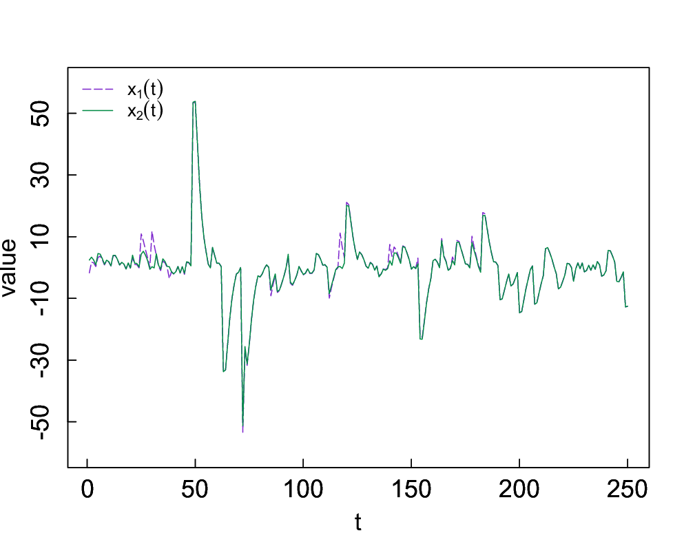
As above, we confirm that our first main claim is certainly satisfied. This claim signifies that a conditional Lyapunov exponent is expressed as the ensemble average of the set of unique Lyapunov exponents of the auxiliary dynamical system. Figure 3 illustrates that two different trajectories with different initial points () partially synchronize. The coupling parameter is . Note that although the conditional Lyapunov exponent is positive in FIG. 3, the partial synchronization occurs since it is the averaged factor of unique Lyapunov exponents. When the conditional Lyapunov exponent is negative, the infinitesimal synchronization error converges to for (see FIG. 4).

IV Example2 for the first claim
Our analysis is not restricted to the above example. We consider another solvable chaotic dynamical system, and can also confirm that the conditional Lyapunov exponent in the system is obtained by Eq. (6). This dynamical system is defined as follows:
The chaotic mapping is associated with the double formula [20]. Its Lyapunov exponent is , and the invariant measure obeys the standard Cauchy distribution. Then, the invariant distribution and the conditional Lyapunov exponent , and the threshold are given as:
where is the positive number which satisfies the following equation:
V Example for the second claim
Here, as for the second claim, the conditional Lyapunov exponent for a system (1) is characterized by only two factors, a dynamical system associated with and a distribution of external forcing input .
In order to show this claim we consider six different dynamical systems. Each of them has a different chaotic mapping or different system for as follows:
where Crand is a set of random numbers which follow . The algorithm to get Crand follows:
where are uniform random numbers on the interval .
We compare the conditional Lyapunov exponent of these systems with Table 1.
| Generation Mechanism of | Lyapunov exponent of | The invariant distribution of the system | the property of time series in external forcing input | ||||
|---|---|---|---|---|---|---|---|
| chaotic | |||||||
| chaotic | |||||||
| Crand(0,1) | random | ||||||
| chaotic | |||||||
| chaotic | |||||||
| Crand(0,1) | random |
As we can see from the Table 1, we can find that some factors do not influence the conditional Lyapunov exponent such as the property of time series in external forcing input. Then, we show that the conditional Lyapunov exponent is characterized by the original mapping and the distribution of external forcing input . The original dynamical system is changed to the system which has an attracting fixed point because of the external forcing input. The conditional Lyapunov exponent is changed by the existence of attracting fixed points. Figures 6 and 6 illustrate that the mappings and are changed to ones that have attracting fixed points by external forcing input respectively.


Attractors of systems depend on how attracting fixed points are generated. The created attractor leads to the -dependence of . Figures 8 and 8 show the set of Lyapunov exponents and that of , respectively. Hence, the original mappings determine how attracting fixed points are generated. Furthermore, with Eq. (6) from the first claim, the conditional Lyapunov exponent is calculated by the set of Lyapunov exponents and the distribution of the external forcing input .


As above, the conditional Lyapunov exponent in system (1) is uniquely characterized by only two factors, the original dynamical system and the distribution of external forcing input.
VI Conclusion
We have two main claims. First, the conditional Lyapunov exponent is expressed as Eq. (6) provided the ergodicity in dynamical systems. This yields that the conditional Lyapunov exponent is expressed as the ensemble average of the set of unique Lyapunov exponents of the auxiliary dynamical system (9). Second, the conditional Lyapunov exponent is characterized only two factors, an original dynamical system and a distribution of external forcing input. Then, although we consider CS in one-dimensional unidirectionally coupled dynamical systems only, this claim will also hold in multi-dimensional chaotic systems in terms of ergodic theory.
Acknowledgements.
The authors thank Shin-itiro Goto (Kyoto University) for stimulating discussions.References
- [1] H. Fujisaka, T. Yamada, Prog. Theor. Phys. 69, 32 (1983)
- [2] L. M. Pecora, T. L. Carroll, Phys. Rev. Lett. 64, 821 (1990)
- [3] L. Kocarev, U. Parlitz, Phys. Rev. Lett. 74, 5028 (1995)
- [4] L. Kocarev, U. Parlitz, Phys. Rev. Lett. 76, 1816 (1996)
- [5] L. Yu, E. Ott, Q. Chen, Phys. Rev. Lett. 65, 2935 (1990).
- [6] A. S. Pikovsky, J. Kurths, Phys. Rev. Lett. 78, 775 (1997)
- [7] A. S. Pikovsky, M. G. Rosenblum, G. V. Osipov, J. Kurths, Physica D: Nonlinear Phenomena 104, 219 (1997)
- [8] A. Pikovsky, M. Rosenblum, J. Kruths, Synchronization A Universal Concept in Nonlinear Sciences, (Cambridge University Press, Cambridge, 2001)
- [9] S. Boccaletti, J. Bragard, F. T. Arecchi, H. Mancini, Phys. Rev. Lett. 83, 536 (1999)
- [10] S. Boccaletti, J. Kurths, G. Osipov, D. Valladares, and C. Zhou, Physics reports 366, 1 (2002)
- [11] S. Rim, D. U. Hwang, I. Kim, C. M. Kim, Phys. Rev. Lett. 85, 2304 (2000)
- [12] G. Shuguang, L. Ying-Cheng, L. C-H and G. Xiaofeng, Phys. Lett. A, 353, 1, 30 (2006)
- [13] C-H. Lai, C. Zhou, EPL. 43, 4, 376 (1998)
- [14] A. Balanov, N. Janson, D. Postnov, O. Sonsnovtseva, Synchronization: From Simple to Complex, (2008)
- [15] S. Goto, K. Yoshimura, P Davis, IEICE Trans. Fundamentals, 91-A, 2535 (2008)
- [16] S. Sunada, K. Arai, K. Yoshimura, M. Adachi, Phys. Rev. Lett. 112, 204101 (2014)
- [17] A. Uchida, K. Umeno, National Congress of Theoretical and Applied Mechanics, 55, 79 (2006) (In Japanese)
- [18] V. I. Oseledets, Trudy Mosk. Matem. 19, 179 (1968)
- [19] K. Umeno, Phys. Rev. E. 55, 5280 (1997)
- [20] K. Umeno, Phys. Rev. E. 58, 2644 (1998)
- [21] K. Umeno and K. Okubo, Prog. Theor. Phys. 2016, 2, 021A01 (2016)
- [22] M. Shintani, K. Umeno, IEICE Technical Report, CCS, 115(178), 11 (2015) (In Japanese)
- [23] K. Umeno, IEICE-NOLTA , 7, 14 (2016)
Appendix A Ergodic dynamical systems
In this Appendix a short introduction of ergodic theory is provided. Since this appendix aims at providing clear definitions of terminologies used in the main text, this appendix is not comprehensive. For a comprehensive review from a mathematical viewpoint (see Refs.[1, 2]), also from a physical viewpoint (see Ref.[3]).
Definition A.1.
(Dynamical system, [1]): A dynamical system is a measure-space equipped with a one-parameter group of automorphisms (except for spaces of measure-zero) of , depending measurably of . Here the parameter denotes an integer.
Given a dynamical system , it follows that , where is a measurable set, and that is a measurable in . In what follows is assumed.
The following average often appears in physics.
Definition A.2.
(Time-average, [1]): Let be a dynamical system, and a complex-valued function defined on . If there exists the quantity
then is called the time-average of .
Also the following average often appears and is related to the time-average for some dynamical systems.
Definition A.3.
(Space-average, [1]): Let be a dynamical system, and a complex-valued function defined on . If there exists the quantity
then is called the space-average of .
Space-average defined above is called ensemble average in the main text. The following is used in the main text.
Definition A.4.
(Absolutely continuous function with respect to the Lebesgue measure): In Definition A.3, if is of the form
then is called an absolutely continuous function with respect to the Lebesgue measure .
We are now ready to state the definition of ergodic system.
Definition A.5.
(Ergodic system, [1]): Let be a dynamical system. If the following condition is satisfied
for any integrable function in the sense of , then the dynamical system is called an ergodic system.
This states that for an ergodic dynamical system, one can replace the time-average of with the space-average of it. An example of how to apply this property is Eq. (4) in the main text.
The following property is a stronger property for dynamical systems.
Definition A.6.
(Mixing system, [1]): Let be a dynamical system. If the condition
is satisfied for all measurable set and ,
then the dynamical system is called a mixing system.
Appendix B Three Properties
In this Appendix, we describe the Properties 2 and 3 in Section III in the main text in more detail. About the Property 2, we get in Section III-A as follows:
This shows that the mapping changes the median and the scale parameter of the input Cauchy distribution as:
| median | ||||
| scale parameter |
We utilize the Properties 1-3 to get Eq. (15). When the variables which follow a Cauchy distribution in the dynamical system Eq. (13), the variables which also follow a Cauchy distribution as Fig. 9.
Hence, we get the self-consistent recurrence equations Eq. (15) about a median and a scale parameter per iteration. This idea is also utilized to get in Section III-C.
References
- [1] V.I. Arnold and A. Avez, “Ergodic problems of classical mechanics”, Benjamin, (1968).
- [2] A. Boyarrsky, and P. Góra, “Laws of chaos”, Birkhäuser, (1997).
- [3] J.-P. Eckmann and D. Ruelle, “Ergodic theory of chaos and strange attractors”, Rev. Mod. Phys. 57, 617–656, (1985).