Graph Structure Learning from Unlabeled Data for Event Detection
Abstract
Processes such as disease propagation and information diffusion often spread over some latent network structure which must be learned from observation. Given a set of unlabeled training examples representing occurrences of an event type of interest (e.g., a disease outbreak), our goal is to learn a graph structure that can be used to accurately detect future events of that type. Motivated by new theoretical results on the consistency of constrained and unconstrained subset scans, we propose a novel framework for learning graph structure from unlabeled data by comparing the most anomalous subsets detected with and without the graph constraints. Our framework uses the mean normalized log-likelihood ratio score to measure the quality of a graph structure, and efficiently searches for the highest-scoring graph structure. Using simulated disease outbreaks injected into real-world Emergency Department data from Allegheny County, we show that our method learns a structure similar to the true underlying graph, but enables faster and more accurate detection.
Keywords: graph learning, event detection, disease surveillance, spatial scan statistic
1 Introduction
Event detection in massive data sets has applications to multiple domains, such as information diffusion or detecting disease outbreaks. In many of these domains, the data has an underlying graph or network structure: for example, an outbreak might spread via person-to-person contact, or the latest trends might propagate through a social network. In the typical, graph-based event detection problem, we are given a graph structure and a time series of observed counts for each graph node , and must detect connected subgraphs where the recently observed counts are significantly higher than expected. For example, public health officials wish to achieve early and accurate detection of emerging outbreaks by identifying connected regions (e.g., subsets of spatially adjacent zip codes ) with anomalously high counts of disease cases.
Assuming that the graph structure is known, various graph-based event detection methods (Patil and Taillie, 2004) can be used to detect anomalous subgraphs. We review these methods in §1.1 below. Typically, however, the network structure is unknown. For example, the spread of disease may be influenced not only by spatial adjacency but also by commuting patterns (e.g., individuals work downtown but live in a suburb), contamination of food or water sources, animal migrations, or other factors. Assuming an incorrect graph structure can result in less timely and less accurate event detection, since the affected areas may be disconnected and hence may not be identified as an anomalous subgraph. In such cases, learning the correct graph structure (e.g., from historical data) has the potential to dramatically improve detection performance.
Thus we consider the graph-based event detection problem in the case where the true graph structure is unknown and must be inferred from data. To learn the graph, we are given a set of training examples , where each example represents a different “snapshot” of the data when an event is assumed to be occurring in some subset of nodes that is connected given the (unknown) graph structure. We assume that training examples are generated from some underlying distribution on the true latent graph structure, and wish to accurately detect future events drawn from that same distribution. Thus our goal is to learn a graph structure that minimizes detection time and maximizes accuracy when used as an input for event detection.
Several recent methods (Gomez-Rodriguez et al., 2010; Myers and Leskovec, 2010; Gomez-Rodriguez and Schölkopf, 2012) learn an underlying graph structure using labeled training data, given the true affected subset of nodes for each training example . However, in many cases labeled data is unavailable: for example, public health officials might be aware that an outbreak has occurred, but may not know which areas were affected and when. Hence we focus on learning graph structure from unlabeled data, where the affected subset of nodes for each training example is not given, and we observe only the observed and expected counts at each node. In the remainder of this paper, we present a novel framework for graph structure learning from unlabeled data, and show that the graphs learned by our approach enable more timely and more accurate event detection. We support these empirical evaluations with new theoretical results on the consistency of constrained and unconstrained subset scans, as described in §3 and §4.4 below.
1.1 Graph-Based Event Detection
Given a graph and the observed and expected counts at each graph node, existing methods for graph-based event detection can be used to identify the most anomalous connected subgraph. Here we focus on the spatial scan framework for event detection, which was first developed by Kulldorff (1997), building on work by Naus (1965) and others, and extended to graph data by Patil and Taillie (2004). These methods maximize the log-likelihood ratio statistic over connected subgraphs . Searching over connected subgraphs, rather than clusters of fixed shape such as circles (Kulldorff, 1997) or rectangles (Neill and Moore, 2004), can increase detection power and accuracy for irregularly shaped spatial clusters.
In this paper, we assume that the score function is an expectation-based scan statistic (Neill et al., 2005). The null hypothesis assumes that no events are occurring, and thus each observed count is assumed to be drawn from some distribution with mean equal to the expected count : . The alternative hypothesis assumes that counts in subgraph are increased by some constant multiplicative factor : for , and for , where is chosen by maximum likelihood estimation. We further assume that Dist is some distribution in the separable exponential family (Neill, 2012), such as the Poisson, Gaussian, or exponential. This assumption enables efficient identification of the highest-scoring connected subgraph and highest-scoring unconstrained subset, which will be important components of our graph structure learning framework described below. Our evaluation results below assume the expectation-based Poisson statistic (Neill et al., 2005). In this case, the log-likelihood ratio score can be computed as , if , and 0 otherwise, where and .
Maximizing the log-likelihood ratio statistic over connected subgraphs is a challenging computational problem for which multiple algorithmic approaches exist. The two main methods we consider in this paper are GraphScan (Speakman et al., 2015b) and Upper Level Sets (ULS) (Patil and Taillie, 2004). GraphScan is guaranteed to find the highest-scoring connected subgraph for the expectation-based scan statistics considered here, but can take exponential time in the worst case. ULS scales quadratically with graph size, but is a heuristic that is not guaranteed to find the optimal subgraph. GraphScan requires less than a minute of computation time for a 100 node graph, and improves detection power as compared to ULS, but is computationally infeasible for graphs larger than to nodes (Speakman et al., 2015b). We also note that the previously proposed FlexScan method (Tango and Takahashi, 2005) identifies subgraphs nearly identical to those detected by GraphScan, but is computationally infeasible for graphs larger than 30 nodes.
As shown by Speakman et al. (2015b), the detection performance of GraphScan and ULS is often improved by incorporating proximity as well as connectivity constraints, thus preventing these methods from identifying highly irregular tree-like structures. To do so, rather than performing a single search over the entire graph, we perform separate searches over the “local neighborhood” of each of the graph nodes, consisting of that node and its nearest neighbors for some constant . We then report the highest-scoring connected subgraph over all local neighborhoods.
2 Problem Formulation
Our framework for graph learning takes as input a set of training examples , assumed to be independently drawn from some
distribution . For each example , we are given the observed count and expected count for each graph node , . We assume that each training example has an set of affected nodes that is a connected subgraph of the true underlying graph
structure ; note that both the true graph and the subgraphs are unobserved. Unaffected nodes are assumed to have
counts that are drawn from some distribution with mean , while affected nodes are assumed to have higher counts. Given
these training examples, we have three main goals:
1) Accurately estimate the true underlying graph structure . Accuracy of graph learning is measured by the precision and recall of the learned set of graph edges as compared to the true graph .
2) Given a separate set of test examples drawn from , identify the affected subgraphs . Accuracy of detection is measured by the average overlap coefficient between the true and identified subgraphs.
3) Distinguish test examples drawn from from examples with no affected subgraph (). Detection power is measured by the true positive rate (proportion of correctly identified test examples) for a fixed false positive rate (proportion of incorrectly identified null examples).
The second and third performance measures assume that the learned graph is used as an input for a graph-based event detection method such as GraphScan, and that
method is used to identify the highest scoring connected subgraph of for each test example.
A key insight of our graph learning framework is to evaluate the quality of each graph structure ( denotes number of edges in the graph) by comparing the most anomalous subsets detected with and without the graph constraints. For a given training example , we can use the fast subset scan (Neill, 2012) to identify the highest-scoring unconstrained subset , with score . This can be done very efficiently, evaluating a number of subsets that is linear rather than exponential in the number of graph nodes, for any function satisfying the linear-time subset scanning property (Neill, 2012), including the expectation-based scan statistics considered here. We can use either GraphScan (Speakman et al., 2015b) or ULS (Patil and Taillie, 2004) to estimate the highest-scoring connected subgraph , with score . We then compute the mean normalized score , averaged over all training examples, as a measure of graph quality.
As noted above, we assume that the affected subset of nodes for each training example is a connected subgraph of the true (unknown) graph structure . Intuitively, if a given graph is similar to , then the maximum connected subgraph score will be close to the maximum unconstrained subset score for many training examples, and will be close to 1. On the other hand, if graph is missing essential connections, then we expect the values of to be much lower than the corresponding , and will be much lower than 1. Additionally, we would expect a graph with high scores on the training examples to have high power to detect future events drawn from the same underlying distribution. However, any graph with a large number of edges will also score close to the maximum unconstrained score. For example, if graph is the complete graph on nodes, all subsets are connected, and for all training examples , giving . Such under-constrained graphs will produce high scores even when data is generated under the null hypothesis, resulting in reduced detection power. Thus we wish to optimize the tradeoff between higher mean normalized score and lower number of edges . Our solution is to compare the mean normalized score of each graph structure to the distribution of mean normalized scores for random graphs with the same number of edges , and choose the graph with the most significant score given this distribution.
3 Theoretical Development
In this section, we provide a theoretical justification for using the mean
normalized score, , as a measure of the quality of graph . Our key result is a proof that the expected value if and only if graph contains the
true graph , assuming a sufficiently strong and homogeneous signal. More precisely, let us assume the following:
(A1) Each training example has an affected subset that is a connected subgraph of . Each is an independent random draw from some distribution , where
each connected subgraph is assumed to have some non-zero probability of being affected.
(A2) The score function is an expectation-based scan statistic in the separable exponential family. Many distributions, such as the Poisson, Gaussian, and exponential, satisfy this property.
Now, for a given training example , we define the observed excess risk for each node .
Let
and denote the maximum and minimum of the observed excess risk over affected nodes, and denote the
maximum of the observed excess risk over unaffected nodes, respectively. We say that the signal for training example is -strong if and only if ,
and we say that the signal for training example is -homogeneous if and only if .
We also define the signal size for training example , . Given assumptions (A1)-(A2) above, we can show:
Lemma 1.
For each training example , there exists a constant such that, if the signal is -homogeneous and 1-strong, then the highest scoring unconstrained subset . We note that is a function of , and for the Poisson, Gaussian, and exponential distributions.
Lemma 2.
For each training example , there exists a constant such that, if the signal is -strong, then the highest scoring unconstrained subset . We note that is a function of , and for the Gaussian distribution.
Proofs of Lemma 1 and Lemma 2 are provided in the Appendix.
Theorem 1.
If the signal is -homogeneous and -strong for all training examples , then the following properties hold for the assumed graph and true graph :
a) If then .
b) If then .
Proof.
Lemmas 1 and 2 imply that for all . For part a), implies that the affected subgraph (which is assumed to be connected in ) is connected in as well. Thus , and for all . For part b), implies that there exists some pair of nodes such that and are connected in but not in . By assumption (A1), the subset has non-zero probability of being generated, and we know , but since the subset is not connected in . Since the signal is -homogeneous and -strong, we observe that is the unique optimum. Thus we have for that training example, and . ∎
4 Learning Graph Structure
We can now consider the mean normalized score as a measure of graph quality, and for each number of edges , we can search for the graph with highest mean normalized score. However, it is computationally infeasible to search exhaustively over all graphs. Even computing the mean normalized score of a single graph may require a substantial amount of computation time, since it requires calling a graph-based event detection method such as Upper Level Sets (ULS) or GraphScan to find the highest-scoring connected subgraph for each training example . In our general framework for graph structure learning, we refer to this call as BestSubgraph(, ), for a given graph structure and training example . Either ULS or GraphScan can be used to implement BestSubgraph, where ULS is faster but approximate, and GraphScan is slower but guaranteed to find the highest-scoring connected subgraph. In either case, to make graph learning computationally tractable, we must minimize the number of calls to BestSubgraph, both by limiting the number of graph structures under consideration, and by reducing the average number of calls needed to evaluate a given graph.
Thus we propose a greedy framework for efficient graph structure learning that starts with the complete graph on nodes and sequentially removes edges until no edges remain (Algorithm 1). This procedure produces a sequence of graphs , for each from down to 0. For each graph , we produce graph by considering all possible edge removals and choosing the one that maximizes the mean normalized score. We refer to this as BestEdge(, ), and consider three possible implementations of BestEdge in §4.1 below. Once we have obtained the sequence of graphs , we can then use randomization testing to choose the most significant graph , as described in §4.2. The idea of this approach is to remove unnecessary edges, while preserving essential connections which keep the maximum connected subgraph score close to the maximum unconstrained subset score for many training examples.
However, a naive implementation of greedy search would require calls to BestSubgraph, since graph structures would be evaluated for each graph to choose the next edge for removal. Even a sequence of random edge removals would require calls to BestSubgraph, to evaluate each graph . Our efficient graph learning framework improves on both of these bounds, performing exact or approximate greedy search with or calls to BestSubgraph respectively. The key insight is that removal of an edge only requires us to call BestSubgraph for those examples where removing that edge disconnects the highest scoring connected subgraph. See §4.3 for further analysis and discussion.
4.1 Edge Selection Methods
Given a graph with edges, we consider three methods for choosing the next edge to remove, resulting in the next graph . First, we consider an exact greedy search. We compute the mean normalized score resulting from each possible edge removal , and choose the edge which maximizes . As noted above, computation of the mean normalized score for each edge removal is made efficient by evaluating the score only for training examples where removing edge disconnects the highest scoring subgraph. The resulting graph will have as close as possible to . We show in §4.3 that only of the candidate edge removals will disconnect the highest scoring subgraphs, reducing the number of calls to BestSubgraph from quartic to cubic in . However, this still may result in overly long run times, necessitating the development of the alternative approaches below.
In the early stages of the greedy edge removal process, when the number of remaining edges is large, many different edge removals might not disconnect any of the subgraphs , and all such graphs would have the same mean normalized score . To avoid removing potentially important edges, we must carefully consider how to break ties in mean normalized score. In this case, we choose the edge with lowest correlation between the counts at nodes and . If two nodes are connected to each other in the latent graph structure over which an event spreads, we expect both nodes to often be either simultaneously affected by an event in that part of the network, or simultaneously unaffected by an event in some other part of the network, and hence we expect the observed counts in these nodes to be correlated. Hence, if the Pearson correlation between two nodes and is very low, the probability that the two nodes are connected is small, and thus edge can be removed. We refer to the resulting algorithm, removing the edge which reduces the mean normalized score the least, and using correlation to break ties, as the Greedy Correlation (GrCorr) method.
Our second approach is based on the observation that GrCorr would require calls to BestSubgraph for each graph , , which may be computationally infeasible depending on the graph size and the implementation of BestSubgraph. Instead, we use the fact that if removing edge does not disconnect subgraph , and otherwise. To do so, we count the number of subgraphs , for , which would be disconnected by removing each possible edge from graph , and choose the which disconnects the fewest subgraphs. The resulting graph is expected to have a mean normalized score which is close to , since for many subgraphs, but this approach does not guarantee that the graph with highest mean normalized score will be found. However, because we choose the edge for which the fewest subgraphs are disconnected, and only need to call BestSubgraph for those examples where removing disconnects , we are choosing the edge which requires the fewest calls to BestSubgraph for each graph . Again, correlation is used to break ties: if two edge removals disconnect the same number of subgraphs, the edge with lower correlation is removed. We refer to this as Pseudo-Greedy Correlation (PsCorr), and we show in §4.3 that this approach reduces the number of calls to BestSubgraph from to as compared to exact greedy search.
In our empirical results below, we compare GrCorr and PsCorr to a simple implementation of , which we refer to as Correlation (Corr). Corr chooses the next edge removal to be the edge with the lowest value of , and hence the greedy edge removal approach corresponds to keeping all edges with correlation above some threshold . Our empirical results, presented below, demonstrate that GrCorr and PsCorr significantly improve timeliness and accuracy of event detection as compared to Corr.
4.2 Finding the Most Significant Graph
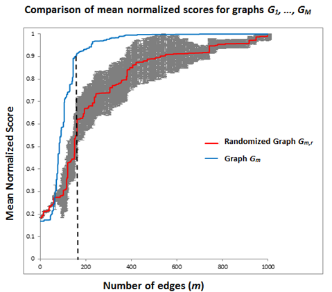
Our proposed graph structure learning approach considers a set of nested graphs , , where graph has edges and is formed by removing an edge from graph . We note that, for this set of graphs, is monotonically increasing with , since the highest scoring connected subgraph for graph will also be connected for graph , and thus for each training example . Our goal is to identify the graph with the best tradeoff between a high mean normalized score and a small number of edges , as shown in Figure 1. Our solution is to generate a large number of random permutations of the edges of the complete graph on nodes. For each permutation , we form the sequence of graphs by removing edges in the given random order, and compute the mean normalized score of each graph. For a given number of edges , we compute the mean and standard deviation of the mean normalized scores of the random graphs with edges. Finally we choose the graph . This “most significant graph” has the most anomalously high value of given its number of edges . Ideally, in order to compute the most significant graph structure, we want to compare our mean normalized score to the mean normalized score of any random graph with the same number of edges. However, due to the computational infeasibility of scoring all the random graph structures with varying number of edges, we instead choose random permutations of edges to be removed.
4.3 Computational Complexity Analysis
We now consider the computational complexity of each step of our graph structure learning framework (Alg. 1), in terms of the number of nodes , number of training examples , and number of randomly generated sequences . Step 1 (computing correlations) requires time for each of the pairs of nodes. Step 2 (computing the highest-scoring unconstrained subsets) requires time for each of the training examples, using the linear-time subset scanning method (Neill, 2012) for efficient computation. Steps 5-10 are repeated times for the original sequence of edges and times for each of the randomly generated sequences of edges. Within the loop, the computation time is dominated by steps 5 and 7, and depends on our choice of and .
For each call to BestSubgraph, GraphScan requires worst-case exponential time, approximately based on empirical results by Speakman et al. (2015b), while the faster, heuristic ULS method requires only time. In step 7, BestSubgraph could be called up to times for each graph structure, for each of the randomly generated sequences of edge removals, resulting in a total of calls. However, BestSubgraph is only called when the removal of an edge disconnects the highest scoring connected subgraph for that graph and training example . We now consider the sequence of edge removals for graphs , where , and compute the expected number of calls to BestSubgraph for these edge removals. We focus on the case of random edge removals, since these dominate the overall runtime for large .
For a given training example , let denote the number of nodes in the highest-scoring connected subgraph for graph , and let denote any spanning tree of . We note that the number of edges in is , which is . Moreover, any edge that is not in will not disconnect , and thus the probability of disconnecting for a random edge removal is upper bounded by the ratio of the number of disconnecting edges to the total number of edges . Thus the expected number of calls to BestSubgraph for graphs for the given training example is = = = . Hence the expected number of calls to BestSubgraph needed for all training examples is for the given sequence of graphs , and for the random sequences of edge removals.
Finally, we consider the complexity of choosing the next edge to remove (step 5 of our graph structure learning framework). The BestEdge function is called times for the given sequence of graphs , but is not called for the random sequences of edge removals. For the GrCorr and PsCorr methods, for each graph and each training example , we must evaluate all candidate edge removals. This requires a total of checks to determine whether removal of each edge disconnects the highest scoring connected subgraph for each graph and training example . The GrCorr method must also call BestSubgraph whenever the highest scoring subgraph is disconnected. However, for a given graph and training example , we show that only of the candidate edge removals can disconnect the highest scoring subset, thus requiring only calls to BestSubgraph rather than . To see this, let be the number of nodes in the highest-scoring connected subgraph , and let be any spanning tree of . Then any edge that is not in will not disconnect , and only has edges.
4.4 Consistency of Greedy Search
The greedy algorithm described above is not guaranteed to recover the true graph structure . However, we can show that, given a sufficiently strong and homogeneous signal, and sufficiently many training examples, the true graph will be part of the sequence of graphs identified by the greedy search procedure. More precisely, let us make assumptions (A1) and (A2) given in §3 above. We also assume that GraphScan (GS) or Upper Level Sets (ULS) is used for BestSubgraph, and that Greedy Correlation (GrCorr) or Pseudo-Greedy Correlation (PsCorr) is used for selecting the next edge to remove (BestEdge). Given these assumptions, we can show:
Theorem 2.
If the signal is -homogeneous and -strong for all training examples , and if the set of training examples is sufficiently large, then the true graph will be part of the sequence of graphs identified by Algorithm 1.
Proof.
Given an -homogeneous and -strong signal, both GS and ULS will correctly identify the highest-scoring connected subgraph . This is true for GS in general, since an exact search is performed, and also true for ULS since will be one of the upper level sets considered. Now let denote the number of edges in the true graph , and consider the sequence of graphs , , …, identified by the greedy search procedure. For each of these graphs , the next edge to be removed (producing graph ) will be either an edge in or an edge in . We will show that an edge in is chosen for removal at each step. Given assumptions (A1)-(A2) and an -homogeneous and -strong signal, Theorem 1 implies:
a) For any graph that contains all edges of the true graph (), we will have for all , and thus .
b) For any graph that does not contain all edges of the true graph, and for any training example drawn from , there is a non-zero probability that we will have , , and thus .
We further assume that the set of training examples is sufficiently large so that every pair of nodes in is the affected subgraph for at least one training example ; note that assumption (A1) ensures that each such pair will be drawn from with non-zero probability. This means that removal of any edge in will disconnect for at least one training example , leading to and , while removal of any edge in will not disconnect for any training examples, maintaining . Hence for both GrCorr, which removes the edge that maximizes , and PsCorr, which removes the edge that disconnects for the fewest training examples, the greedy search procedure will remove all edges in before removing any edges in , leading to . ∎
5 Related Work
We now briefly discuss several streams of related work. As noted above, various spatial scan methods have been proposed for detecting the most anomalous subset in data with an underlying, known graph structure, including Upper Level Sets (Patil and Taillie, 2004), FlexScan (Tango and Takahashi, 2005), and GraphScan (Speakman et al., 2015b), but none of these methods attempt to learn an unknown graph structure from data. Link prediction algorithms such as (Taskar et al., 2004; Vert and Yamanishi, 2005) start with an existing network of edges and attempt to infer additional edges which might also be present, unlike our scenario which requires inferring the complete edge structure. Much work has been done on learning the edge structure of graphical models such as Bayesian networks and probabilistic relational models (Getoor et al., 2003), but these methods focus on understanding the dependencies between multiple attributes rather than learning a graph structure for event detection. Finally, the recently proposed NetInf (Gomez-Rodriguez et al., 2010), ConNIe (Myers and Leskovec, 2010), and MultiTree (Gomez-Rodriguez and Schölkopf, 2012) methods share our goal of efficiently learning graph structure. NetInf is a submodular approximation algorithm for predicting the latent network structure and assumes that all connected nodes influence their neighbors with equal probability. ConNIe relaxes this assumption and uses convex programming to rapidly infer the optimal latent network, and MultiTree is an extension of NetInf which considers all possible tree structures instead of only the most probable ones. The primary difference of the present work from NetInf, ConNIe, and MultiTree is that we learn the underlying graph structure from unlabeled data: while these methods are given the affected subset of nodes for each time step of an event, thus allowing them to learn the network edges along which the event spreads, we consider the more difficult case where we are given only the observed and expected counts at each node, and the affected subset of nodes is not labeled. Further, these methods are not targeted towards learning a graph structure for event detection, and we demonstrate below that our approach achieves more timely and accurate event detection than MultiTree, even when MultiTree has access to the labels.
6 Experimental Setup
In our general framework, we implemented two methods for : GraphScan (GS) and Upper Level Sets (ULS). We also implemented three methods for : GrCorr, PsCorr, and Corr. However, using GraphScan with the true greedy method (GS-GrCorr) was computationally infeasible for our data, requiring 3 hours of run time for a single 50-node graph, and failing to complete for larger graphs. Hence our evaluation compares five combinations of BestSubgraph and BestEdge: GS-PsCorr, GS-Corr, ULS-GrCorr, ULS-PsCorr, and ULS-Corr.
We compare the performance of our learned graphs with the learned graphs from MultiTree, which was shown to outperform previously proposed graph structure learning algorithms such as NetInf and ConNIe (Gomez-Rodriguez and Schölkopf, 2012). We used the publicly available implementation of the algorithm, and considered both the case in which MultiTree is given the true labels of the affected subset of nodes for each training example (MultiTree-Labels), and the case in which these labels are not provided (MultiTree-NoLabels). In the latter case, we perform a subset scan for each training example , and use the highest-scoring unconstrained subset as an approximation of the true affected subset.
6.1 Description of Data
Our experiments focus on detection of simulated disease outbreaks injected into real-world Emergency Department (ED) data from ten hospitals in Allegheny County, Pennsylvania. The dataset consists of the number of ED admissions with respiratory symptoms for each of the zip codes for each day from January 1, 2004 to December 31, 2005. The data were cleaned by removing all records where the admission date was missing or the home zip code was outside the county. The resulting dataset had a daily mean of 44.0 cases, with a standard deviation of 12.1.
6.2 Graph-Based Outbreak Simulations
Our first set of simulations assume that the disease outbreak starts at a randomly chosen location and spreads over some underlying graph structure, increasing in size and severity over time. We assume that an affected node remains affected through the outbreak duration, as in the Susceptible-Infected contagion model (Bailey, 1975). For each simulated outbreak, we first choose a center zip code uniformly at random, then order the other zip codes by graph distance (number of hops away from the center for the given graph structure), with ties broken at random. Each outbreak was assumed to be 14 days in duration. On each day of the outbreak (), we inject counts into the nearest zip codes, where , and is a parameter which determines how quickly the inject spreads. For each affected node , we increment the observed count by , where , and is a parameter which determines how quickly the inject severity decreases with distance. The assumption of Poisson counts is common in epidemiological models of disease spread; the expected number of injected cases is an increasing function of the inject day , and a decreasing function of the graph distance between the affected node and the center of the outbreak. We considered 4 different inject types, as described below; for each type, we generated training injects (for learning graph structure) and an additional 200 test injects to evaluate the timeliness and accuracy of event detection given the learned graph.
6.2.1 Zip code adjacency graph based injects
We first considered simulated outbreaks which spread from a given zip code to spatially adjacent zip codes, as is commonly assumed in the literature. Thus we formed the adjacency graph for the 97 Allegheny County zip codes, where two nodes are connected by an edge if the corresponding zip codes share a boundary. We performed two sets of experiments: for the first set, we generated simulated injects using the adjacency graph, while for the second set, we added additional edges between randomly chosen nodes to simulate travel patterns. As noted above, a contagious disease outbreak might be likely to propagate from one location to another location which is not spatially adjacent, based on individuals’ daily travel, such as commuting to work or school. We hypothesize that inferring these additional edges will lead to improved detection performance.
6.2.2 Random graph based injects
Further, in order to show that we can learn a diverse set of graph structures over which an event spreads, we performed experiments assuming two types of random graphs, Erdos-Renyi and preferential attachment. For each experiment, we used the same set of nodes consisting of the 97 Allegheny County zip codes, but created a random set of edges connecting these nodes; the graph was then used to simulate 200 training and 200 test outbreaks, with results averaged over multiple such randomly chosen graphs.
First, we considered Erdos-Renyi graphs (assuming that each pair of nodes is connected with a constant probability ), with edge probabilities ranging from 0.08 to 0.20. The relative performance of methods was very similar across different values, and thus only the averaged results are reported. Second, we considered preferential attachment graphs, scale-free network graphs which are constructed by adding nodes sequentially, assuming that each new node forms an edge to each existing node with probability proportional to that node’s degree. We generated the preferential attachment graph by first connecting three randomly chosen nodes, then adding the remaining nodes in a random order. Each new node that arrives attaches itself to each existing node with probability , where each node’s maximum degree was restricted to .
6.3 Simulated Anthrax Bio-Attacks
We present additional evaluation results for one potentially realistic outbreak scenario, an increase in respiratory Emergency Department cases resulting from an airborne release of anthrax spores (e.g. from a bio-terrorist attack). The anthrax attacks are based on a state-of-the-art, highly realistic simulation of an aerosolized anthrax release, the Bayesian Aerosol Release Detector (BARD) simulator (Hogan et al., 2007). BARD uses a combination of a dispersion model (to determine which areas will be affected and how many spores people in these areas will be exposed to), an infection model (to determine who will become ill with anthrax and visit their local Emergency Department),and a visit delay model to calculate the probability of the observed Emergency Department visit counts over a spatial region. These complex simulations take into account weather data when creating the affected zip codes and demographic information when calculating the number of additional Emergency Department cases within each affected zip code. The weather patterns are modeled with Gaussian plumes resulting in elongated, non-circular regions of affected zip codes. Wind direction, wind speed, and atmospheric stability all influence the shape and size of the affected area. A total of 82 simulated anthrax attacks were generated and injected into the Allegheny County Emergency Department data, using the BARD model. Each simulation generated between 33 and 1324 cases in total (mean = 429.2, median = 430) over a ten-day outbreak period; half of the attacks were used for training and half for testing.
7 Experimental Results
7.1 Computation Time
For each of the experiments described above (adjacency, adjacency plus travel patterns, Erdos-Renyi random graphs, and preferential attachment graphs), we report the average computation time required for each of our methods (Table 1). Randomization testing is not included in these results, since it is not dependent on the choice of BestEdge. Each sequence of randomized edge removals required 1 to 2 hours for the GraphScan-based methods and 1 to 3 minutes for the ULS-based methods.
| Experiment | GraphScan (GS) | ULS | MultiTree | ||||
|---|---|---|---|---|---|---|---|
| PsCorr | Corr | GrCorr | PsCorr | Corr | Labels | NoLabels | |
| Adjacency | 41 | 38 | 13 | 2 | 1 | 1 | 1 |
| Adjacency+Travel | 53 | 47 | 15 | 3 | 1 | 1 | 1 |
| Erdos-Renyi (avg) | 93 | 89 | 22 | 6 | 3 | 1 | 1 |
| Pref. Attachment | 49 | 44 | 17 | 3 | 1 | 1 | 1 |
| Size | GraphScan (GS) | ULS | MultiTree | ||||
|---|---|---|---|---|---|---|---|
| PsCorr | Corr | GrCorr | PsCorr | Corr | Labels | NoLabels | |
| N=50 | 2 | 2 | 1 | 1 | 1 | 1 | 1 |
| N=75 | 37 | 32 | 3 | 1 | 1 | 1 | 1 |
| N=100 | 58 | 53 | 13 | 3 | 1 | 1 | 1 |
| N=200 | - | - | 91 | 33 | 1 | 1 | 1 |
| N=500 | - | - | 2958 | 871 | 27 | 2 | 2 |
For each of the training examples, all methods except for ULS-GrCorr required fewer than 80 calls to BestSubgraph on average to search over the space of graph structures, a reduction of nearly two orders of magnitude as compared to the naive approach of calling BestSubgraph for each combination of graph structure and training example. Similarly, a naive implementation of the true greedy search would require approximately 11 million calls to BestSubgraph for each training example, while our ULS-GrCorr approach required only 5000 calls per training example, a three order of magnitude speedup. As expected, ULS-Corr and ULS-PsCorr had substantially faster run times than GS-Corr and GS-PsCorr, though the GraphScan-based approaches were still able to learn each graph structure in less than two hours.
Next, in order to evaluate how each method scales with the number of nodes , we generated Erdos-Renyi random graphs with edge probability and ranging from 50 to 500. For each graph, we generated simulated counts and baselines, as well as simulating injects to produce training examples for learning the graph structure. Table 2 shows the average time in minutes required by each method to learn the graph structure. We observe that the ULS-based methods were substantially faster than the GraphScan-based methods, and were able to scale to graphs with nodes, while GS-Corr and GS-PsCorr were not computationally feasible for . We note that MultiTree has much lower computation time as compared to our graph learning methods, since it is not dependent on calls to a graph-based event detection method (BestSubgraph); however, its detection performance is lower, as shown below in our experiments.
7.2 Comparison of True and Learned Graphs
For each of the four graph-based injects (adjacency, adjacency plus travel patterns, Erdos-Renyi, and preferential attachment), we compare the learned graphs to the true underlying graph over which the simulated injects spread. Table 3 compares the number of edges in the true underlying graph to the number of edges in the learned graph structure for each of the methods, and Tables 4 and 5 show the precision and recall of the learned graph as compared to the true graph. Given the true set of edges and the learned set of edges , the edge precision and recall are defined to be and respectively. High recall means that the learned graph structure identifies a high proportion of the true edges, while high precision means that the learned graph does not contain too many irrelevant edges. We observe that GS-PsCorr had the highest recall, with nearly identical precision to GS-Corr and ULS-GrCorr. MultiTree had higher precision and comparable recall to GS-PsCorr when it was given the true labels, but 3-5% lower precision and recall when the labels were not provided.
| Experiment | Edges | Learned Edges | ||||||
|---|---|---|---|---|---|---|---|---|
| (true) | GraphScan (GS) | ULS | MultiTree | |||||
| PsCorr | Corr | GrCorr | PsCorr | Corr | Labels | NoLabels | ||
| Adjacency | 216 | 319 | 297 | 305 | 332 | 351 | 280 | 308 |
| Adjacency+Travel | 280 | 342 | 324 | 329 | 362 | 381 | 316 | 342 |
| Erdos-Renyi () | 316 | 388 | 369 | 359 | 398 | 412 | 356 | 382 |
| Pref. Attachment | 374 | 394 | 415 | 401 | 428 | 461 | 399 | 416 |
| Experiment | Precision | ||||||
|---|---|---|---|---|---|---|---|
| GraphScan (GS) | ULS | MultiTree | |||||
| PsCorr | Corr | GrCorr | PsCorr | Corr | Labels | NoLabels | |
| Adjacency | 0.60 | 0.62 | 0.62 | 0.53 | 0.50 | 0.66 | 0.58 |
| Adjacency+Travel | 0.70 | 0.71 | 0.69 | 0.60 | 0.52 | 0.75 | 0.65 |
| Erdos-Renyi (avg) | 0.56 | 0.59 | 0.61 | 0.59 | 0.54 | 0.62 | 0.56 |
| Pref. Attachment | 0.83 | 0.79 | 0.80 | 0.69 | 0.59 | 0.86 | 0.80 |
| Experiment | Recall | ||||||
|---|---|---|---|---|---|---|---|
| GraphScan (GS) | ULS | MultiTree | |||||
| PsCorr | Corr | GrCorr | PsCorr | Corr | Labels | NoLabels | |
| Adjacency | 0.89 | 0.86 | 0.88 | 0.81 | 0.77 | 0.86 | 0.83 |
| Adjacency+Travel | 0.86 | 0.83 | 0.81 | 0.77 | 0.71 | 0.85 | 0.79 |
| Erdos-Renyi (avg) | 0.87 | 0.81 | 0.83 | 0.79 | 0.70 | 0.84 | 0.79 |
| Pref. Attachment | 0.88 | 0.81 | 0.86 | 0.79 | 0.73 | 0.91 | 0.89 |
7.3 Comparison of Detection Performance
We now compare the detection performance of the learned graphs on the test data: a separate set of 200 simulated injects (or injects for the BARD anthrax simulations), generated from the same distribution as the training injects which were used to learn that graph. To evaluate a graph, we use the GraphScan algorithm (assuming the given graph structure) to identify the highest-scoring connected subgraph and its likelihood ratio score for each day of each simulated inject, and for each day of the original Emergency Department data with no cases injected. We note that performance was substantially improved by using GraphScan for detection as compared to ULS, regardless of whether GraphScan or ULS was used to learn the graph, and GraphScan required less than a few seconds of run time for detection per day of the ED data.
We then evaluate detection performance using two metrics: average time to detection (assuming a false positive rate of 1 fp/month, typically considered acceptable by public health), and spatial accuracy (overlap between true and detected clusters). To compute detection time, we first compute the score threshold for detection at 1 fp/month. This corresponds to the 96.7th percentile of the daily scores from the original ED data. Then for each simulated inject, we compute the first outbreak day with ; for this computation, undetected outbreaks are counted as days (maximum number of inject days) to detect. We then average the time to detection over all 200 test injects. To evaluate spatial accuracy, we compute the average overlap coefficient between the detected subset of nodes and the true affected subset at the midpoint (day 7) of the outbreak, where overlap is defined as .
As noted above, detection performance is often improved by including a proximity constraint, where we perform separate searches over the “local neighborhood” of each of the graph nodes, consisting of that node and its nearest neighbors, and report the highest-scoring connected subgraph over all neighborhoods. We compare the detection performance of each graph structure by running GraphScan with varying neighborhood sizes for each outbreak type.
7.3.1 Results on zip code adjacency graphs
We first evaluate the detection time and spatial accuracy of GraphScan, using the learned graphs, for simulated injects which spread based on the adjacency graph formed from the 97 Allegheny County zip codes, as shown in Figure 2. This figure also shows the performance of GraphScan given the true zip code adjacency graph. We observe that the graphs learned by GS-PsCorr and ULS-GrCorr have similar spatial accuracy to the true zip code adjacency graph, as measured by the overlap coefficient between the true and detected subsets of nodes, while the graphs learned by GS-Corr and MultiTree have lower spatial accuracy. Surprisingly, all of the learned graphs achieve more timely detection than the true graph: for the optimal neighborhood size of , ULS-GrCorr and GS-PsCorr detected an average of 1.4 days faster than the true graph. This may be because the learned graphs, in addition to recovering most of the edges of the adjacency graph, also include additional edges to nearby but not spatially adjacent nodes (e.g. neighbors of neighbors). These extra edges provide added flexibility to consider subgraphs which would be almost but not quite connected given the true graph structure. This can improve detection time when some nodes are more strongly affected than others, enabling the strongly affected nodes to be detected earlier in the outbreak before the entire affected subgraph is identified. Finally, ULS-GrCorr and GS-PsCorr detected 0.6 days faster than MultiTree for .
 |
 |
 | |
 |
 |
 | |
7.3.2 Results on adjacency graphs with simulated travel patterns
Next we compared detection time and spatial accuracy, using the graphs learned by each of the methods, for simulated injects which spread based on the zip code adjacency graph with additional random edges added to simulate travel patterns, as shown in Figure 3. This figure also shows the detection performance given the true (adjacency plus travel) graph and the adjacency graph without travel patterns. We observe again that GS-PsCorr and ULS-GrCorr achieve similar spatial accuracy to the true graph, while the original adjacency graph, GS-Corr, and MultiTree have lower spatial accuracy. Our learned graphs are able to detect outbreaks 0.8 days earlier than MultiTree, 1.2 days earlier than the true graph, and 1.7 days earlier than the adjacency graph without travel patterns. This demonstrates that our methods can successfully learn the additional edges due to travel patterns, substantially improving detection performance.
7.3.3 Results on random graphs
 |
 |
| |
 |
 |
| |
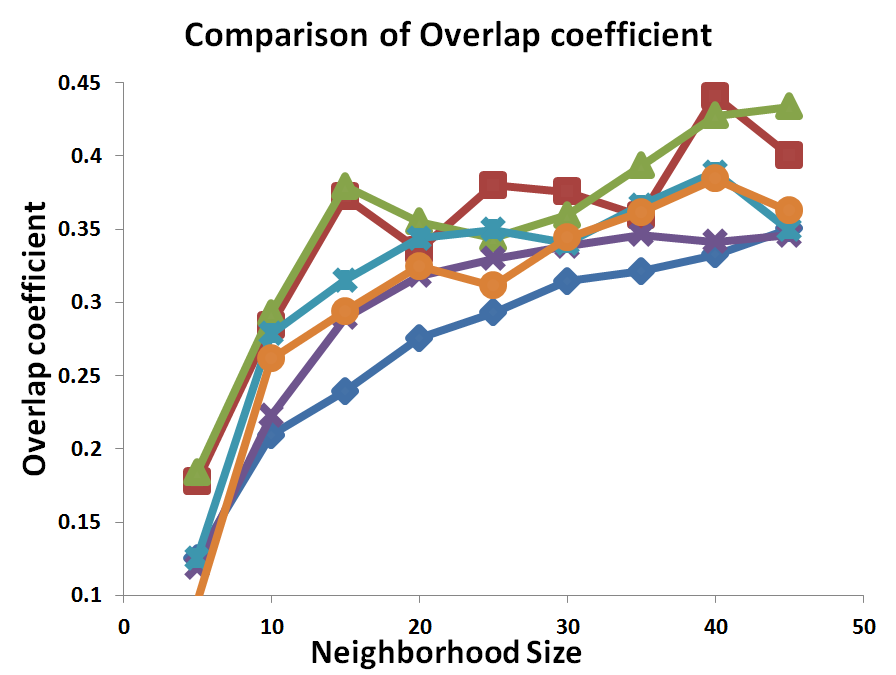
Next we compared detection time and spatial accuracy using the learned graphs for simulated injects which spread based on Erdos-Renyi and preferential attachment graphs, as shown in Figures 4 and 5 respectively. Each figure also shows the performance of the true randomly generated graph. As in the previous experiments, we observe that our learned graphs achieve substantially faster detection than the true graph and MultiTree. For preferential attachment, the learned graphs also achieve higher spatial accuracy than the true graph, with GS-PsCorr and ULS-GrCorr again outperforming GS-Corr and MultiTree. For Erdos-Renyi, GS-PsCorr and ULS-GrCorr achieve similar spatial accuracy to the true graph, while GS-Corr and MultiTree have lower accuracy.
7.3.4 Results on BARD simulations
We further compared the detection time and spatial accuracy using learned graphs based on realistic simulations of anthrax bio-attacks, as shown in Figure 6. In these simulations there is no “true” graph structure as these were generated using spatial information based on environmental characteristics (wind direction, etc.). Hence, we compare the performance of various graphs learned or assumed. It can be seen that the learned graphs using GS-PsCorr and ULS-GrCorr achieve substantially faster detection and higher spatial accuracy, as compared to assuming the adjacency graph and the graphs learned using GS-Corr and MultiTree.
 |
 |
 | |
7.4 Effect of number of training examples on performance
All of the experiments discussed above (except for the BARD simulations) assume unlabeled training examples for learning the graph structure. We now evaluate the graphs learned by two of our best performing methods, GS-PsCorr and ULS-GrCorr, using smaller numbers of training examples ranging from to . Simulated outbreaks were generated based on the preferential attachment graph described in §6.2.2. As shown in Figure 7, GS-PsCorr and ULS-GrCorr perform very similarly both in terms of average number of days to detect and spatial accuracy. Performance of both methods improves with increasing training set size, outperforming the true graph structure for .
 |
 |
 | |
7.5 Effect of percentage of injects in training data on performance
All of the experiments discussed above (except for the BARD simulations) assume that the unlabeled training examples are each a “snapshot” of the observed count data at each node during a time when an event is assumed to be occurring. However, in practice the training data may be noisy, in the sense that some fraction of the training examples may be from time periods where no events are present. Thus we evaluate performance of the graphs learned by GS-PsCorr and ULS-GrCorr (for simulated outbreaks based on the preferential attachment graph described in §6.2.2) using a set of training examples, where proportion of the examples are based on simulated inject data, and proportion are drawn from the original Emergency Department data with no outbreaks injected. As shown in Figure 8, the performance of both GS-PsCorr and ULS-GrCorr improves as the proportion of injects in the training data increases. For , both methods achieve more timely detection than the true underlying graph, with higher spatial accuracy. These results demonstrate that our graph structure learning methods, while assuming that all training examples contain true events, are robust to violations of this assumption.
 |
 |
| |
8 Conclusions and Future Work
In this work, we proposed a novel framework to learn graph structure from unlabeled data, based on comparing the most anomalous subsets detected with and without the graph constraints. This approach can accurately and efficiently learn a graph structure which can then be used by graph-based event detection methods such as GraphScan, enabling more timely and more accurate detection of events (such as disease outbreaks) which spread based on that latent structure. Within our general framework for graph structure learning, we compared five approaches which differed both in the underlying detection method (BestSubgraph) and the method used to choose the next edge for removal (BestEdge), incorporated into a provably efficient greedy search procedure. We demonstrated both theoretically and empirically that our framework requires fewer calls to BestSubgraph than a naive greedy approach, as compared to for exact greedy search, and as compared to for approximate greedy search, resulting in 2 to 3 orders of magnitude speedup in practice.
We tested these approaches on various types of simulated disease outbreaks, including outbreaks which spread according to spatial adjacency, adjacency plus simulated travel patterns, random graphs (Erdos-Renyi and preferential attachment), and realistic simulations of an anthrax bio-attack. Our results demonstrated that two of our approaches, GS-PsCorr and ULS-GrCorr, consistently outperformed the other three approaches in terms of spatial accuracy, timeliness of detection, and accuracy of the learned graph structure. Both GS-PsCorr and ULS-GrCorr consistently achieved more timely and more accurate event detection than the recently proposed MultiTree algorithm (Gomez-Rodriguez and Schölkopf, 2012), even when MultiTree was provided with labeled data not available to our algorithms. We observed a tradeoff between scalability and detection: GS-PsCorr had slightly better detection performance than ULS-GrCorr, while ULS-GrCorr was able to scale to larger graphs (500 nodes vs. 100 nodes). None of our approaches are designed to scale to massive graphs with millions of nodes (e.g. online social networks); they are most appropriate for moderate-sized graphs where labeled data is not available and timely, accurate event detection is paramount.
In general, our results demonstrate that the graph structures learned by our framework are similar to the true underlying graph structure, capturing nearly all of the true edges but also adding some additional edges. The resulting graph achieves similar spatial accuracy to the true graph, as measured by the overlap coefficient between true and detected clusters. Interestingly, the learned graph often has better detection power than the true underlying graph, enabling more timely detection of outbreaks or other emerging events. This result can be better understood when we realize that the learning procedure is designed to capture not only the underlying graph structure, but the characteristics of the events which spread over that graph. Unlike previously proposed methods, our framework learns these characteristics from unlabeled training examples, for which we assume that an event is occurring but are not given the affected subset of nodes. By finding graphs where the highest connected subgraph score is consistently close to the highest unconstrained subset score when an event is occurring, we identify a graph structure which is optimized for event detection. Our ongoing work focuses on extending the graph structure learning framework in several directions, including learning graph structures with directed rather than undirected edges, learning graphs with weighted edges, and learning dynamic graphs where the edge structure can change over time.
Acknowledgments
This work was partially supported by NSF grants IIS-0916345, IIS-0911032, and IIS-0953330. Preliminary work was presented at the 2011 International Society for Disease Surveillance Annual Conference, with a 1-page abstract published in the Emerging Health Threats Journal. This preliminary work did not include the theoretical developments and results, the computational algorithmic advances, and the large set of comparison methods and evaluations considered here.
Appendix A Proofs of Lemma 1 and Lemma 2
We begin with some preliminaries which will be used in both proofs. Following the notation in Neill (2012), we write the distributions from the exponential family as , where is the sufficient statistic, is a function mapping the mean to the natural parameter , is the log-partition function, and is the convex conjugate of . By assumption (A2), is an expectation-based scan statistic in the separable exponential family, defined by Neill (2012) as follows:
Definition 1.
The separable exponential family is a subfamily of the exponential family such that , where the function depends only on , while and can depend on and but are independent of .
Such functions can be written in the form , where:
Speakman et al. (2015a) have shown that is a concave function with global maximum at and zeros at and , where and is an increasing function of . Considering the corresponding excess risks and , we know:
| (1) |
where is the average value of between 1 and .
From this equation, it is easy to see that when is concave, as is the case for the Poisson, Gaussian, and exponential distributions, with , , and respectively. For the Gaussian, since is linear, while for the Poisson and exponential.
Further, the assumption of an expectation-based scan statistic in the separable exponential family (A2) implies that the score function satisfies the linear-time subset scanning property (Neill, 2012) with priority function . This means that the highest-scoring unconstrained subset can be found by evaluating the score of only of the subsets of nodes, that is, for some between 1 and , where represents the th highest-priority node.
Given the set of all nodes sorted by priority, we note that the assumption of a 1-strong signal implies that the true affected subset , where is the cardinality of . Thus, for Lemma 1 we need only to show that , while for Lemma 2 we must show . We can now prove:
See 1
Proof.
Let , where is the function defined in Equation (1) above. For distributions with concave , such as the Poisson, Gaussian, and exponential, we know that , and thus . Now, the assumption of -homogeneity implies , , and since is an increasing and therefore invertible function, .
Now we note that is the observed excess risk for the lowest-priority affected node , where is the cardinality of , while is the observed excess risk for the highest-priority affected node . Moreover, the contribution of node to the log-likelihood ratio statistic, , will be positive for all , and we know that the maximum likelihood estimate of for any subset of nodes will be at most . Thus node will make a positive contribution to the log-likelihood ratio and will be included in , as will nodes . Hence , and . ∎
See 2
Proof.
Let , where is the inverse of the function defined in Equation (1) above. For distributions with convex , such as the Gaussian, we know that , and thus . Now, the assumption that the signal is -strong, where , implies and thus .
Now we note that is the observed excess risk for the lowest-priority affected node , and is the observed excess risk for the highest-priority unaffected node , where is the cardinality of . Moreover, the contribution of node to the log-likelihood ratio statistic, , will be negative for all . Finally, we know that the maximum likelihood estimate of for any will be at least , where , where the key step is to lower bound each by for and by 0 for respectively. Thus node will make a negative contribution to the log-likelihood ratio and will be excluded from , as will nodes . Hence , and . ∎
References
- Bailey (1975) Bailey, N. T. J. (1975). The mathematical theory of infectious diseases and its applications. Hafner Press.
- Getoor et al. (2003) Getoor, L., Friedman, N., Koller, D., and Taskar, B. (2003). Learning probabilistic models of link structure. J. Mach. Learn. Res., 3, 679–707.
- Gomez-Rodriguez et al. (2010) Gomez-Rodriguez, M., Leskovec, J., and Krause, A. (2010). Inferring networks of diffusion and influence. In Proc. 16th ACM SIGKDD Intl. Conf. on Knowledge Discovery and Data Mining, pages 1019–1028.
- Gomez-Rodriguez and Schölkopf (2012) Gomez-Rodriguez, M. G. and Schölkopf, B. (2012). Submodular inference of diffusion networks from multiple trees. In Proc. 29th Intl. Conf. on Machine Learning, pages 489–496.
- Hogan et al. (2007) Hogan, W. R., Cooper, G. F., Wallstrom, G. L., Wagner, M. M., and Depinay, J. M. (2007). The Bayesian aerosol release detector: an algorithm for detecting and characterizing outbreaks caused by atmospheric release of Bacillus anthracis. Stat. Med., 26, 5225–52.
- Kulldorff (1997) Kulldorff, M. (1997). A spatial scan statistic. Communications in Statistics: Theory and Methods, 26(6), 1481–1496.
- Myers and Leskovec (2010) Myers, S. and Leskovec, J. (2010). On the convexity of latent social network inference. In Advances in Neural Information Processing Systems 23, pages 1741–1749.
- Naus (1965) Naus, J. I. (1965). The distribution of the size of the maximum cluster of points on the line. Journal of the American Statistical Association, 60, 532–538.
- Neill (2012) Neill, D. B. (2012). Fast subset scan for spatial pattern detection. Journal of the Royal Statistical Society (Series B: Statistical Methodology), 74(2), 337–360.
- Neill and Moore (2004) Neill, D. B. and Moore, A. W. (2004). Rapid detection of significant spatial clusters. In Proc. 10th ACM SIGKDD Conf. on Knowledge Discovery and Data Mining, pages 256–265.
- Neill et al. (2005) Neill, D. B., Moore, A. W., Sabhnani, M. R., and Daniel, K. (2005). Detection of emerging space-time clusters. In Proc. 11th ACM SIGKDD Intl. Conf. on Knowledge Discovery and Data Mining, pages 218–227.
- Patil and Taillie (2004) Patil, G. P. and Taillie, C. (2004). Upper level set scan statistic for detecting arbitrarily shaped hotspots. Envir. Ecol. Stat., 11, 183–197.
- Speakman et al. (2015a) Speakman, S., Somanchi, S., McFowland III, E., and Neill, D. B. (2015a). Penalized fast subset scanning. Journal of Computational and Graphical Statistics, (in press).
- Speakman et al. (2015b) Speakman, S., McFowland III, E., and Neill, D. B. (2015b). Scalable detection of anomalous patterns with connectivity constraints. Journal of Computational and Graphical Statistics, (in press).
- Tango and Takahashi (2005) Tango, T. and Takahashi, K. (2005). A flexibly shaped spatial scan statistic for detecting clusters. International Journal of Health Geographics, 4, 11.
- Taskar et al. (2004) Taskar, B., Wong, M.-F., Abbeel, P., and Koller, D. (2004). Link prediction in relational data. In Advances in Neural Information Processing Systems 16, pages 659–666.
- Vert and Yamanishi (2005) Vert, J.-P. and Yamanishi, Y. (2005). Supervised graph inference. In Advances in Neural Information Processing Systems 17, pages 1433–1440.