Applying DCOP to User Association Problem in Heterogeneous Networks with Markov Chain Based Algorithm

The definitions of DCOP have a little difference in different literatures [26, 4, 5] ¹¹ 1 [26] formalized the DCOP as a three tuples model. [4] adopted a four-tuples model while [5] used a five tuples model. In this paper, we formalize the DCOP as a four tuples model $<\mathcal{A},\mathcal{V},\mathcal{D},\mathcal{C}>$ where $\mathcal{A}=\{a_{1},a_{2},...,a_{\lvert\mathcal{A}\rvert}\}$ consists of a set of agents, $\mathcal{V}=\{v_{1},v_{2},...,v_{n}\}$ is the set of variables in which each variable $v_{i}\in\mathcal{V}$ only belongs to an agent $a\in\mathcal{A}$. Each variable has a finite and discrete domain where each value represents a possible state of the variable. All the domains of different variables consist of a domain set $\mathcal{D}=\{d_{1},d_{2},...,d_{n}\}$, where $d_{i}$ is the domain of $v_{i}$. A constraint $c\in\mathcal{C}=\{c_{1},c_{2},...,c_{\lvert\mathcal{C}\rvert}\}$ is defined as a mapping from the assignments of $m$ variables to a positive real value:

The purpose of a DCOP is to find a set of assignments of all the variables, denoted as $\mathcal{X}^{*}$, which maximize the utility, namely the sum of all constraint rewards:

Consider a $k$-tier HetNet where all the BSs in the same tier have the same configurations. For example, a two-tier network including a macro BS ($\mathcal{B}_{1}$) and a femto BS, ($\mathcal{B}_{2}$), is shown in Fig.1. The set of all BSs is denoted as $\mathcal{B}=\{\mathcal{B}_{1},\mathcal{B}_{2},...,\mathcal{B}_{\mathcal{NB}}\}$ where $\mathcal{NB}$ is the total number of BSs. All the BSs in the $k$th tier transmit with the same power $P_{k}$. The total number of users is denoted by $\mathcal{NU}$ and the set of all users is $\mathcal{U}=\{\mathcal{U}_{1},\mathcal{U}_{2},...,\mathcal{U}_{\mathcal{NU}}\}$.

With OFDMA technology in LTE-Advanced networks, the resource, time-frequency, is divided into blocks where each block is defined as a resource block (RB) including a certain time duration and certain bandwidth [17]. In this paper, the resource configured at each BS is in the format of RB so that its available RBs are decided by the bandwidth and the scheduling interval duration allocated to that BS. We assume the BSs in the HetNet share the total bandwidth such that both intra- and inter-tier interference exist when the BSs allocate RBs to the users instantaneously.

Assuming the channel state information is available at the BSs, the ${\rm SINR}$ experienced by user $\mathcal{U}_{j}$, served by $\mathcal{B}_{i}$ in the $k$th tier is given by

In (3), $g_{ij}$ is the channel power gain between $\mathcal{U}_{j}$ and $\mathcal{B}_{i}$, $\mathcal{B}/\{\mathcal{B}_{i}\}$ represents all the BSs in $\mathcal{B}$ except $\mathcal{B}_{i}$, $B$ is the bandwidth and $N_{0}$ is noise power spectral density. The channel power gain includes the effect of both path loss and fading. Path loss is assumed to be static and its effect is captured in the average value of the channel power gain, while the fading is assumed to follow the exponential distribution.

From the above, the efficiency of user $\mathcal{U}_{j}$ powered by BS $\mathcal{B}_{i}$, denoted as $e_{ij}$, is calculated as

Given the bandwidth $B$, time duration $T$ and the scheduling interval $\varGamma$ configured at each RB, we attain the unit rate at $\mathcal{U}_{j}$ upon one RB as follows

On the basis of formula (5), the rate received at $\mathcal{U}_{j}$ with $n_{ij}$ RBs provided by $\mathcal{B}_{i}$ in the $k$th tier is

Associated with each user is a quality-of-service (QoS) constraint. This is expressed as the minimum total rate the user should receive. Denoting the rate requiremnt of the $j$th user by $\gamma_{j}$, the minimum number of RBs required to satisfy $\gamma_{j}$ is calculated by:

The formulations of user association problem by mixed linear programming are similar in a series of papers (see the survey literature [19]). in this paper, we present a more commonly used formulation as follows

The first constraint ensures the rate QoS requirement from users. Constraint (8c) indicates that the amount of RBs consumed at the same BS is no more than the total RBs $N_{i}$ configurated at the BS. Constraint (8d) guarantees one user associated with a unique BS. Constraint (8e) guarantees the number of RBs a BS allocates to a user falls within the range from zero and $N_{i}$. The last constraint (8f) guarantees the connection between a user and a BS has two states denoted by a binary variable. The objective function (8a) refers to the sum of rate rather than a function acted on the rate such as $U(x_{ij}r_{ij})$ (e.g. $U(x)=log(1+x)$) in some references. Generally, two phases are needed to gain the solution including: 1) transforming original problem into a satisfied one through relaxing Constraint (8e) by $n_{ij}\in\{0,n_{min}^{ij}\}$; 2) the left RBs in each BS will be allocated to users in order to maximize the objective function.

Before giving the formulation based on DCOP, we firstly introduce the definition of candidate BS:

After confirming the set of candidate BSs of $\mathcal{U}_{j},j\in\mathcal{U}$, denoted by, $\mathcal{CB}_{j}$, $\mathcal{U}_{j}$ sends messages to its candidate BSs so that each $\mathcal{B}_{i},i\in\mathcal{NB}$ gets knowledge of its possible connected users. We define each possible connection between $\mathcal{U}_{j}$ and its candidate BS $\mathcal{B}_{i}$ as a variable, denoted by $\mathcal{V}_{i}^{j}$. In this case, all the variables are divided into $\mathcal{NB}$ groups according to the potential connection between users and different BSs. The domain of each variable $\mathcal{V}_{i}^{j}$, denoted by $\mathcal{D}_{i}^{j}=\{0,n_{min}^{ij},...,N_{i}\}$, where $\mathcal{V}_{i}^{j}=0$ if no RB is allocated to $\mathcal{U}_{j}$, otherwise, $\mathcal{V}_{i}^{j}\geqslant n_{min}^{ij}$. We define each group as an agent. Thus, an $n$-ary constraint exists among $n$ variables (intra-constraint) to guarantee that there is no overload at $\mathcal{B}_{i}$. Note that a user may have more than one candidate BS, there are constraints (inter-constraints) connecting the variables affiliated to different agents on account of the assumption that a unique connection exists between a user and a BS. Generally speaking, the utility (objective) function in the DCOP model is the sum of constraint rewards which reflects the degree of constraint violations. We define the reward $R(c)$ of inter- and intra-constraints in the ECAV model as follows. For $\forall c\in\mathcal{C}_{inter}$

In constraint (9a), $\psi(c)$ is the subset of variables connected by constraint $c$. $Val(\mathcal{V}_{i}^{j})$ represents the assignment of $\mathcal{V}_{i}^{j}$. A reward (we use $-\infty$ in this paper) is assigned to the constraints if there at least two variables are non-zero at the same time (unique connection between a user and a BS). Otherwise, the reward is equal to zero. In constraint (10a), the reward is $-\infty$ once there is a overload at the BS. Otherwise, the reward is the sum of the rates achieved at users.

It is easy to find that a variable in the ECAV model with non-zero assignment covers constraint (8b) and (8e) in the mixed integer programming formulation. Moreover, intra and inter-constraints respectively cover constraint (8c) and constraint(8d). Therefore, The global optimal solution $\mathcal{X}^{*}$ obtained from the ECAV model is consistent with the one obtained from the mixed integer programming formulation, denoted as $\mathcal{X}$ ²² 2 We say $\mathcal{X}^{*}$ is consistent with $\mathcal{X}$ when the total rate calculated by objective function (2) and (8a) is equal. This is because there may be no more than one optimal solution..

To better understand the modeling process, we recall the instance in Fig.1 where the candidate BSs of $\mathcal{U}_{1}$ and $\mathcal{U}_{2}$ are the same, denoted as $\{\mathcal{B}_{1},\mathcal{B}_{2}\}$, while the candidate BSs of $\mathcal{U}_{3}$ and $\mathcal{U}_{4}$ are respectively $\{\mathcal{B}_{1}\}$ and $\{\mathcal{B}_{2}\}$. We assume the total RBs configurated at $\mathcal{B}_{1}$ and $\mathcal{B}_{2}$ is 8 and 10. For simplicity, we assume the rate of each user served by one RB provided by $\mathcal{B}_{1}$ is 0.8 bit/s. And 1 bit/s of each user is served by $\mathcal{B}_{2}$. Then, the ECAV model is shown in Fig.1(b). There are two agents named $\mathcal{A}_{1}$ and $\mathcal{A}_{2}$. The variables in $\mathcal{A}_{1}$ are $\mathcal{V}_{1}^{1},\mathcal{V}_{1}^{2}$ and $\mathcal{V}_{1}^{3}$ where $\mathcal{V}_{i}^{j}$ refers to a connection between user $\mathcal{U}_{j}$ and $\mathcal{B}_{i}$. Similarly, the variables in $\mathcal{A}_{2}$ are $\mathcal{V}_{2}^{1},\mathcal{V}_{2}^{2}$ and $\mathcal{V}_{2}^{4}$. Assuming the threshold rate is 3 bit/s, we can calculate that at least $\lceil\frac{3}{0.8}\rceil=4$ RBs needed for the users served by $\mathcal{B}_{1}$, thus the domain of each variable in $\mathcal{A}_{1}$ is $\{0,4,...,8\}$. Also, the domain of each variable in $\mathcal{A}_{2}$ is $\{0,3,...,10\}$. The black lines in each agent are two 3-nry intra-constraints, thus $\mathcal{C}_{intra}=\{\mathcal{C}_{intra}^{1},\mathcal{C}_{intra}^{2}\}$. The red lines connecting two agents are two intra-constraints, thus $\mathcal{C}_{inter}=\{\mathcal{C}_{inter}^{1},\mathcal{C}_{inter}^{2}\}$. We use $\mathcal{C}_{intra}^{1}$ and $\mathcal{C}_{inter}^{1}$ to illustrate how the reward of constraint works in different conditions. Considering $\mathcal{C}_{intra}^{1}$, the reward is $-\infty$ when all the variables associated with $\mathcal{C}_{intra}^{1}$ have the same assignment 4. Thus the total number of RBs consumed by three users is 12 which is more than 8 RBs configurated at $\mathcal{B}_{1}$. Otherwise, the reward is 0.8 $\times$ 4 $\times$ 3 = 9.6 (bit/s) calculated according to (6). Considering $\mathcal{C}_{inter}^{1}$, the reward is $-\infty$ when the assignment of $\mathcal{V}_{2}^{1}$ is 3 and the assignment of $\mathcal{V}_{1}^{1}$ is 4 because it means $\mathcal{U}_{2}$ will connect with more than one BSs ($\mathcal{B}_{1}$ and $\mathcal{B}_{2}$), which violates the assumption of unique connection. Otherwise, the reward is 0 (9b)). If there is no constraint violated, the final utility calculated by the objective function is the total rate in the whole HetNet (constraint (10b)).

The scale of an ECAV model, referring to the number of agents and constraints, is related to the number of users, BSs and the candidate BSs hold at each user. However, some candidate BSs of the user can be ignored because these BSs are able to satisfy the requirement of the user but with massive RBs consumed. It can be illustrated by the number of RBs a BS allocate to a user is inversely proportional to the geographical distance between them. In this way, we introduce a parameter $\eta$ with which we limit the number of candidate BSs of each user is no more than $\eta$. The following algorithms present the selection of top $\eta$ candidate BSs (denoted by $\hat{\mathcal{CB}}$) and the modeling process of ECAV-$\eta$.

Algorithm 1 is the pseudo code for determining $\hat{\mathcal{CB}}$. It is executed by each user distributely. More precisely, a user estimates its total candidate BSs $\mathcal{CB}$ by the procedure from line 5 to 9. Based on 4 to 7, the candidate BSs of a user is ordered according to the unit number of RBs consumed at such user served by different BSs (from line 22 to 28). The time consumption of Algorithm 1 mainly consists of two parts. One is the dermination of $\mathcal{CB}$ with time complexity $O(\mathcal{NB})$. The other is the ordering operation with time complexity $O(\mathcal{NB}^{2})$. As a result, the total time expended of Algorithm 1 is $O(\mathcal{NB}+\mathcal{NB}^{2})$. With $\hat{\mathcal{CB}}$, we present the pseudo code in relation to the building of ECAV-$\eta$ model.

As for Algorithm 2, it firstly sets up the agents distributely (line 6). It takes $O(1)$. After that, each user determines variables, domains as well as inter-constraints from line 8 to 14. This is also carried out in parallel with $O(1)$. Finally, the intra-constraints are constructed by each agent with $O(1)$ (line 16 to 17). The total time complexity is $O(3)$.

In this section, we test the performance of the MC based algorithm with different assginments of $\eta$ in the ECAV model. A simulated environment including a three-tiers HetNet created within a $1000m\times 1000m$ square is considered. In the system, there is one macro BS, 5 pico BSs and 10 femto BSs with their transmission powers respectively 46, 35, and 20 dBm. The macro BS is fixed at the center of the square, and the other BSs are randomly distributed. The path loss between the macro (pico) BSs and the users is defined as $L(d)=34+40log_{10}(d)$, while the pass loss between femto BSs and users is $L(d)=37+30log_{10}(d)$. The parameter $d$ represents the Euclidean distance between the BSs and the users in meters. The noise power refers to the thermal noise at room temperature with a bandwidth of 180kHz and equals to -111.45 dBm. One second scheduling interval is considered. Without special illustration, 200 RBs are configured at macro BS, as well as 100 and 50 RBs are configured at each pico and femto BS. In addition, all the results are the mean of 10 instances.

We firstly discuss the impact of different assignments of $\eta$ on the performance of ECAV model from the point of view of the runtime and the quality of solution. More precisely, we generate different number of users ranging from 20 to 100 with the step interval of 10. The time consumed by the MC based algorithm is displayed in Fig.2. It is clear to see that more time is needed when the number of users increases. Also, the growth of runtime is depended on the value of $\eta$. Specially, there is an explosive growth of runtime when we set $\eta$ from four to five. As previously stated, this is caused by more candidate BSs considered by each user. However, the quality of the solutions with different values of $\eta$ is not obviously improved according the results in Table I. For instance, the average rate achieved at each user is only improved no more than 0.1 bit/s when the number of users are 100 with the values of $\eta$ are 3 and 5. It is difficult to make a theoretical analysis of the realationship between $\eta$ and the quality of the solution. We leave this research in future works.

From above analysis, we set $\eta=3$ in the following experiments in order to balance the runtime and performance of the solution. In addition, we test the performance of the MC based algorithm comparing with its counterparts Max-SINR and LDD based algorithms.

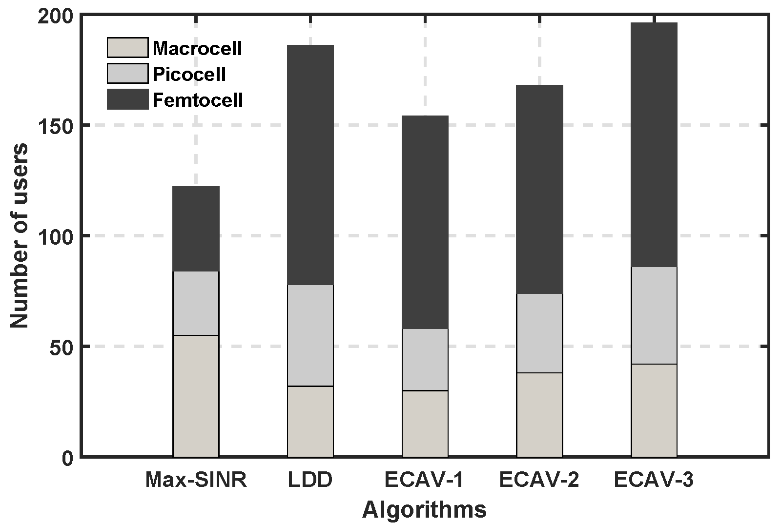
In Fig.3, we check the connection state between 200 users and BSs in different tiers. A phenomenon we can observe from the figure is that there are more or less some users out of service even we use different kinds of algorithms. It is not only caused by the limited resource configured at each BSs, but also related to the positions of such kinds of users. They are located at the edge of the square and hardly served by any BS in the system. Further, more users are served by macro BS in Max-SINR algorithm because a larger SINR always eixsts between the users and macro BS. As a result, the total non-served users in Mmax-SINR algorithms are more than the other two if there is no scheme for allocating the left resource. On the other hand, the number of non-served users in MC are less than LDD when $\eta=3$ since the user $\mathcal{U}_{j}$ will select a BS $\mathcal{B}_{i}$ with the maximal $QI_{ij}$ in each iteration of the LDD algorithm. In other words, the users prefer to connect with a BS which can offer better QoS even when more resources are consumed. Therefore, some BSs have to spend more RBs which leads to the resource at these BSs being more easily used up.

In Fig.4, we produce a statistic of the number of non-served users when we change the total number of users configured in the HetNet. The average number of non-served users for each algorithm along with the standard deviation is presented in the figure. Compared with Fig.3, a more clear results imply that more than 60 (at worst, around 70) non-served users in the Max-SINR algorithm. The LDD based algorithm comes the second with approximate 20 users. The best resutls are obtained by the MC algorithm with no more than 20 users even the total users in the HetNet is 240.

In Fig.5, we compare the cumulative distribution function (CDF) of the rate. The rate of the users seldomly drops below the threshold (3 bit/s) when we use the distributed algorithms (LDD and MC based algorithms), while Max-SINR algorithm is unable to satisfy the rate QoS constraints. Moreover, the rate CDFs of the MC based algorithm never lie above the corresponding CDFs obtained by implementing the Max-SINR algorithm (the gap is between $6\%-20\%$). Likewise, At worst $5\%$ gap eixts between the MC based algorithm and LDD when we set $\eta=3$.

At last, another intesest observation is made by configurating different number of RBs at macro BS (Fig.6). When we change the number of RBs from 150 to 250 at macro BS, it is clear to see that the total rate obtained by LDD is not sensitive to the variation of the resource hold by macro BS. This result is also related to the solving process in which two phases are needed when employing a LDD based algorithm. As we have discuss in the Introduction section, a solution which can satisfy the basic QoS requirement will be accepted by the LDD based algorithm. It finally affects the allocation of left resource at marco BS. As a result, the algorithm easily falls into the local optima. This problem, to some degree, can be overcome by the ECAV model since there is only one phase in the model. With the ECAV model, a constraint satisfied problem is transformed into a constraint optimizaiton problem. And the advantage of DCOP is successfully applied into solving user assocation problem.

References

- [1] F. Fioretto, F. Campeotto, A. Dovier, E. Pontelli, and W. Yeoh, Large neighborhood search with quality guarantees for distributed constraint optimization problems,” in Proceedings of the 2015 International Conference on Autonomous Agents and Multiagent Systems. International Foundation for Autonomous Agents and Multiagent Systems, 2015, pp. 1835–1836.
- [2] F. Fioretto, W. Yeoh, and E. Pontelli, A dynamic programming-based mcmc framework for solving dcops with gpus,” in International Conference on Principles and Practice of Constraint Programming. Springer, 2016, pp. 813–831.
- [3] X. Ge, S. Tu, T. Han, Q. Li, and G. Mao, Energy efficiency of small cell backhaul networks based on gauss–markov mobile models,” IET Networks, vol. 4, no. 2, pp. 158–167, 2015.
- [4] Y. Kim and V. R. Lesser, Djao: A communication-constrained dcop algorithm that combines features of adopt and action-gdl.” in AAAI, 2014, pp. 2680–2687.
- [5] T. Le, F. Fioretto, W. Yeoh, T. C. Son, and E. Pontelli, Er-dcops: A framework for distributed constraint optimization with uncertainty in constraint utilities,” in Proceedings of the 2016 International Conference on Autonomous Agents & Multiagent Systems. International Foundation for Autonomous Agents and Multiagent Systems, 2016, pp. 606–614.
- [6] F. Fioretto, W. Yeoh, and E. Pontelli, Multi-variable agent decomposition for dcops,” in Thirtieth AAAI Conference on Artificial Intelligence, 2016.
- [7] W. Yeoh, P. Varakantham, X. Sun, and S. Koenig, Incremental dcop search algorithms for solving dynamic dcops,” in The 10th International Conference on Autonomous Agents and Multiagent Systems-Volume 3. International Foundation for Autonomous Agents and Multiagent Systems, 2011, pp. 1069–1070.
- [8] V. Lesser, C. L. Ortiz Jr, and M. Tambe, Distributed sensor networks: A multiagent perspective. Springer Science & Business Media, 2012, vol. 9.
- [9] G. Mao and B. D. Anderson, Graph theoretic models and tools for the analysis of dynamic wireless multihop networks,” in 2009 IEEE Wireless Communications and Networking Conference. IEEE, 2009, pp. 1–6.
- [10] G. Mao, B. D. Anderson, and B. Fidan, Online calibration of path loss exponent in wireless sensor networks,” in IEEE Globecom 2006. IEEE, 2006, pp. 1–6.
- [11] A. A. Kannan, B. Fidan, and G. Mao, Robust distributed sensor network localization based on analysis of flip ambiguities,” in IEEE GLOBECOM 2008-2008 IEEE Global Telecommunications Conference. IEEE, 2008, pp. 1–6.
- [12] K. Kinoshita, K. Iizuka, and Y. Iizuka, Effective disaster evacuation by solving the distributed constraint optimization problem,” in Advanced Applied Informatics (IIAIAAI), 2013 IIAI International Conference on. IEEE, 2013, pp. 399–400.
- [13] T. Brys, T. T. Pham, and M. E. Taylor, Distributed learning and multi-objectivity in traffic light control,” Connection Science, vol. 26, no. 1, pp. 65–83, 2014.
- [14] R. Mao and G. Mao, Road traffic density estimation in vehicular networks,” in 2013 IEEE Wireless Communications and Networking Conference (WCNC). IEEE, 2013, pp. 4653–4658.
- [15] F. Amigoni, A. Castelletti, and M. Giuliani, Modeling the management of water resources systems using multi-objective dcops,” in Proceedings of the 2015 International Conference on Autonomous Agents and Multiagent Systems. International Foundation for Autonomous Agents and Multiagent Systems, 2015, pp. 821–829.
- [16] P. Rust, G. Picard, and F. Ramparany, Using message-passing dcop algorithms to solve energy-efficient smart environment configuration problems,” in International Joint Conference on Artificial Intelligence, 2016.
- [17] N. Guan, Y. Zhou, L. Tian, G. Sun, and J. Shi, QoS guaranteed resource block allocation algorithm for lte systems,” in Proc. Int. Conf. Wireless and Mob. Comp., Netw. and Commun. (WiMob), Shanghai, China, Oct. 2011, pp. 307–312.
- [18] T. K. Vu, Resource allocation in heterogeneous networks,” Ph.D. dissertation, University of Ulsan, 2014.
- [19] D. Liu, L. Wang, Y. Chen, M. Elkashlan, K.-K. Wong, R. Schober, and L. Hanzo, User association in 5g networks: A survey and an outlook,” IEEE Communications Surveys & Tutorials, vol. 18, no. 2, pp. 1018–1044, 2016.
- [20] H. Boostanimehr and V. K. Bhargava, Unified and distributed QoS-driven cell association algorithms in heterogeneous networks,” IEEE Wireless Commun., vol. 14, no. 3, pp. 1650–1662, 2015.
- [21] Q. Ye, B. Rong, Y. Chen, C. Caramanis, and J. G. Andrews, Towards an optimal user association in heterogeneous cellular networks,” in Global Communications Conference (GLOBECOM), 2012 IEEE. IEEE, 2012, pp. 4143–4147.
- [22] V. N. Ha and L. B. Le, Distributed base station association and power control for heterogeneous cellular networks,” IEEE Transactions on Vehicular Technology, vol. 63, no. 1, pp. 282–296, 2014.
- [23] T. L. Monteiro, M. E. Pellenz, M. C. Penna, F. Enembreck, R. D. Souza, and G. Pujolle, Channel allocation algorithms for wlans using distributed optimization,” AEU-International Journal of Electronics and Communications, vol. 66, no. 6, pp. 480–490, 2012.
- [24] T. L. Monteiro, G. Pujolle, M. E. Pellenz, M. C. Penna, and R. D. Souza, A multi-agent approach to optimal channel assignment in wlans,” in 2012 IEEE Wireless Communications and Networking Conference (WCNC). IEEE, 2012, pp. 2637–2642.
- [25] J. Xie, I. Howitt, and A. Raja, Cognitive radio resource management using multi-agent systems,” in IEEE CCNC, 2007.
- [26] M. Vinyals, J. A. Rodriguez-Aguilar, and J. Cerquides, Constructing a unifying theory of dynamic programming dcop algorithms via the generalized distributive law,” Autonomous Agents and Multi-Agent Systems, vol. 22, no. 3, pp. 439–464, 2011.
- [27] S. Boyd and L. Vandenberghe, Convex optimization. Cambridge university press, 2004.
- [28] M. Chen, S. C. Liew, Z. Shao, and C. Kai, Markov approximation for combinatorial network optimization,” IEEE Transactions on Information Theory, vol. 59, no. 10, pp. 6301–6327, 2013.
- [29] H. Katagishi and J. P. Pearce, Kopt: Distributed dcop algorithm for arbitrary k-optima with monotonically increasing utility,” in Ninth DCR Workshop, 2007.
- [30] P. J. Modi, W.-M. Shen, M. Tambe, and M. Yokoo, Adopt: Asynchronous distributed constraint optimization with quality guarantees,” Artificial Intelligence, vol. 161, no. 1, pp. 149–180, 2005.