Energy-Efficient Transceiver Design for Hybrid Sub-Array Architecture MIMO Systems
Abstract
Millimeter-wave (mmWave) communication operated in frequency bands between 30 and 300 GHz has attracted extensive attention due to the potential ability of offering orders of magnitude greater bandwidths combined with further gains via beamforming and spatial multiplexing from multi-element antenna arrays. MmWave system may exploit the hybrid analog and digital precoding to achieve simultaneously the diversity, array and multiplexing gain with a lower cost of implementation. Motivated by this, in this paper, we investigate the design of hybrid precoder and combiner with sub-connected architecture, where each radio frequency chain is connected to only a subset of base station (BS) antennas from the perspective of energy efficient transmission. The problem of interest is a non-convex and NP-hard problem that is difficult to solve directly. In order to address it, we resort to design a two-layer optimization method to solve the problem of interest by exploiting jointly the interference alignment and fractional programming. First, the analog precoder and combiner are optimized via the alternating-direction optimization method (ADOM) where the phase shifter can be easily adjusted with an analytical structure. Then, we optimize the digital precoder and combiner based on an effective multiple-input multiple-output (MIMO) channel coefficient. The convergence of the proposed algorithms is proved using the monotonic boundary theorem and fractional programming theory. Extensive simulation results are given to validate the effectiveness of the presented method and to evaluate the energy efficiency performance under various system configurations.
Index Terms:
Millimeter-wave communication, multiple-input multiple-output (MIMO) system, analog precoding and combining, interference alignment, energy efficiency.I Introduction
Recently, data traffic has suffered an exponential growth due to the rapid proliferation of wireless devices, which are creating a spectrum crisis at the current wireless frequency bands. A variety of communication and signal processing techniques are currently being pursued for improvement of wireless rate and efficient use of the available spectrum, such as multiple-input multiple-output (MIMO) technologies [1, 2, 3, 4, 5, 6]. Despite these efforts, meeting the dramatically increasing data demands of wireless devices and applications is still a tremendous challenge for sub-6 Gigabit Hertz wireless communications [7].
Millimeter Wave (mmWave) wireless communication systems, operating in the frequency bands from GHz, are emerging as a promising technology for the exploding bandwidth requirements by enabling multi-Gpbs speeds [8, 9, 10, 11, 12]. Recently, the advance in mmWave hardware has encouraged studying and applying mmWave for outdoor cellular networks and short distance communication. However, the shortcoming is that mmWave signal may experience an order of magnitude increase in free-space path-loss due to the ten-fold increase in carrier frequency compared to sub-6 GHz frequency bands. Fortunately, the decrease in wavelength leads to a dramatic increase of the number of antenna elements within a given antenna size such that large arrays can provide narrow and high-gain beams to overcome the path-loss [13, 14, 15, 16, 17, 18, 19, 20]. Furthermore, large arrays may significantly improve the spectrum efficiency by transmitting simultaneously multiple data streams [21, 22, 25, 23, 24].
Unlike lower frequency MIMO systems, the large arrays combined with high cost and power consumption of the mixed analog/digital signal components makes it difficult to assign an RF chain per antenna, and perform all the signal processing in the baseband. To achieve both the diversity gain and the multiplexing gain in mmWave wireless communication, more recently, the research on the hybrid precoder and combiner have attracted extensive attention from both academia and industry. In such systems, analog beamforming (phase shifters) compensates the large path loss at mmWave bands, while digital beamforming provides the necessary flexibility to perform advanced multiuser MIMO techniques such as multi-streams MIMO. However, the joint design of hybrid precoder and combiner is challenging under a set of practical constraints. Most existing algorithms were designed for the hybrid precoding with fully-connected architecture, where each RF chain is connected to all BS antennas via phase shifters [26, 31, 27, 28, 29, 30, 32].
In recent years, with the rapid development of the mobile communications and the ever growing demand for data rate, the energy consumption problem has become very severe. Particularly with the widespread popularity of smart phones, the problem of battery energy consumption has become a serious constraint for users who wish to experience high-speed data transmission and multimedia services [33, 34, 35, 36, 37]. Li et al investigated the energy efficiency (EE) optimization problem using the double auction theory for relay selection networks [34]. The authors further investigated the EE problem by jointly optimizing the position and serving range of the relay station in [35]. In [36] and [37], the authors investigated the EE optimization problem for coordinated multicell multiuser cellular networks. For the conventional digital precoding [34, 35, 36, 37], each antenna requires a dedicated energy-intensive radio frequency (RF) chain (including digital-to-analog converter, up converter, etc), whose energy consumption is a large part (about 250mW per RF chain [38]) of the total energy consumption for wide bandwidth communication systems.
In this paper, we investigate the energy efficient design of the hybrid precoder and combiner with sub-connected architecture, where each RF chain is connected to only a subset of transmitting antennas, for point-to-point mmWave MIMO wireless communication. The design goal is to maximize the system energy efficiency. We design the analog precoder by resorting the idea of interference alignments. Finally, a two-layer optimization method is designed to solve the problem of interest. The contribution of this paper can be summarized as follows.
- 1.
Inspired by the idea of the interference alignment (IA) for interference channels, the analog precoder and combiner are optimized via the alternating-direction optimization method (ADOM) where the phase shifter can be easily adjusted with an analytical structure.
- 2.
After the analog precoder and combiner are designed, by regarding the sub-array point-to-point communication system as an interference channel, the digital precoder and combiner based on an effective MIMO channel coefficient are optimized.
- 3.
The convergence of the proposed algorithms is proved based on the monotonic boundary theorem and fractional programming theory.
- 4.
Extensive simulation results are provided to validate the effectiveness of the presented method and to evaluate the energy efficiency performance under various system configurations.
The remainder of this paper is organized as follows. The system model is described in Section II. In section III an effective optimization algorithm based on IA is proposed. In Section IV, numerical evaluations of these algorithms are carried out and conclusions are finally drawn in Section V.
The following notations are used throughout this paper. Bold lowercase and uppercase letters represent column vectors and matrices, respectively. The superscripts , and represent the conjugate transpose operator, and the matrix inverse, respectively. and represent the th column and the element of matrix . is the th entry of . denotes the Euclidean norm for vectors and the Frobenius norm of matrix . denotes the phase of . The probability density function (pdf) of a circular complex Gaussian random vector with mean and covariance matrix is denoted as . are the real number field. Expectation is denoted by and the real part of a variable is denoted by .
II System Model
Consider a point-to-point MIMO channel where each transceiver is equipped with a hybrid MIMO processor. For simplicity, assume that the transceivers have transmit/receive RF antenna arrays, where each RF array is fed by a separate RF chain. Each array consists of antenna elements with each connected to one phase shifter. The transmitter has antennas and sends independent data streams to the receiver which is also equipped with antennas and RF chains under the assumption of to assure the feasibility of the degrees of freedom in MIMO channel [3]. The symbols transmitted by the transmitter are processed by a baseband precoder of dimension and then up-converted through RF chains before being precoded by an RF preocder of dimension , as shown in Fig. . It should be pointed out that the baseband precoder enables both amplitude and phase modifications, while only phase changes can be realized by as it is implemented using analog phase shifter [42]. The structure of is given as
| (1) |
where denotes the steering vector of phases for the th antenna array (or RF chain) to point at some given azimuth direction.
flushleft
\onelinecaptionstrue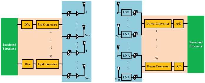
Using these notations, the transmitted signal at the transmitter is denoted as , where is a signal vector of complex information symbol to be transmitted with . For simplicity, considering a narrow block-fading propagation channel [26, 27], then the received signal vector at the receiver is then given by
| (2) |
where is the vector of i.i.d. , denotes the channel coefficients between the transmitter and the receiver with the following structure:
| (3) |
where , , and . Moreover, to enable precoding, we assume that the channel is known perfectly and instantaneously to both the transmitter and receiver. In practical systems, channel state information (CSI) at the receiver can be obtained via training and subsequently shared with the transmitter via limited feedback [22, 25, 26, 27]. In the same way as the transmitter, the steering vector for the th RF array at the receiver is written as the vector , where is the azimuth steering direction for the th RF array at the receiver. Thus, the overall RF combiner at the receiver is given by
| (4) |
Then, the baseband received signal vector at the receiver can be written as
| (5) |
where is the digital combiner at receiver. When Gaussian symbols are transmitted over the mmWave channel, the spectral efficiency achieved is given by [43, 44]
| (6a) | ||||
| (6b) | ||||
where , , . The second equality is based on the fact that .
III Transceiver Design for Maximizing System Energy Efficiency
In this section, we design hybrid mmWave precoder and combiner to maximize the system utility function defined as:
| (7) |
where and are respectively the set of feasible RF precoders at transmitter and receiver, is the power consumption at transceiver and given by
| (8a) | ||||
| (8b) | ||||
| (8c) | ||||
where and represent the power consumed by the RF chain at transmitter and receiver, respectively. and denote respectively the power consumed by the DAC and ADC. , , and denote respectively the power consumed by the power amplifier, the low noise amplifier, the phase shifter, and the baseband processor. is a constant which accounts for the inefficiency of the power amplifier [45]. Note that , then problem () can be rewritten as
| (9) |
and . Unfortunately, the fraction form of the objective and the non-convex constraints on and and the fractional form of the objective lead the optimization to be non-convex [39, 40] and NP-hard [45, 36, 37]. In other words, it is difficult to find globally optimal solution for problem () within polynomial time. In what follows, we will use two steps to solve design the hybrid precoding. First, an alternative optimization RF precoding and combiner scheme is presented using the ideas of the IA used in interference channels [3, 4]. Then, for fixed RF precoding and combiner, we further present an optimization algorithm to solve the energy efficiency problem via the relation between the user rate and the minimum mean square error (MMSE) [53] and the fractional programming theory [39, 40].
III-A Analog Precoder and Combiner Optimization
Without considering the digital baseband precoder and combiner, similar to the interference channel, the analog shifters of the transceiver can be regarded as interference channel networks where the design of precoder at each transmitter aims to minimize the interference leaking to other receivers and put all the interference into the same subspace. Different from the conventional design of the IA algorithm [3, 4], the elements of the analog precoder and combiner are subjected to constant-envelop with only changing of the phase making the problem more intractable [49].
In this subsection we design distributed analog precoder and combiner for the interference channel networks consisted by the analog shifters. In what follows, we start with arbitrary phase shifter and iteratively update phase shifter and with aiming to reduce the leakage of interference. The quality of the analog precoder is measured by the power in the leakage interference at each receiver, i.e., the interference power in the received signal after the analog combiner is applied. The total interference leakage at receive sub-array due to all undesired transmit sub-array () is given by
Similarly, in the reciprocal network, the total interference leakage at receive sub-array due to all undesired transmit sub-array () is given by
In the sequel, we aim to develop an iterative algorithm alternating between the transmitter and receiver to update their analog phase shifter to minimize their total leakage interference. For receive sub-array , we aim to solve the following optimization problem to obtain the receive phase shifter vector.
| (10) |
It is easy to see that the receive sub-array chooses its phase shifter to minimize the leakage interference due to all undesired transmit sub-array (). Unlike the method used in [4], the single eigenvalue decomposition can not be directly used to obtain the phase of the shifter vector. After some basic mathematic manipulation, it is easy to see that the objective in () can be expanded as follows
| (11) |
where is a Hermitian positive semidefinite matrix, and are a column vector of dimension obtained by removing the th entry of and the th entry of , respectively, is a matrix of dimension obtained by removing the th row and th column of matrix . Note that in () the first two item and are independent of the phase applied by the th antenna in the th sub-array. It also means that the dependence of the objective of () on the phase shift of the th antenna in the th sub-array is fully captured in the third item which can be minimized by anti-phasing and . Therefore, to minimize the objective function in () with a constant envelope constraint of phase shifter [26, 27], all elements of the vector must satisfy the following optimization condition
| (12) |
Thus, an algorithm summarized as Algorithm is designed to find the optimal array of phase shifts for fixing where , , and denote respectively the iterative counter, the objective of () and the stop threshold.
Note that in Algorithm , the mathematical operation includes complex multiplication, complex addition and phase operation. Furthermore, each sub-array can simultaneously update its analog beamforming vector that facilitates parallel hardware implementation.
Similarly, for transmit sub-array , we aim to solve the following optimization problem to obtain the receive phase shifters.
| (13) |
Likely, the objective in () can be expanded as follows
| (14) |
where is a Hermitian positive semidefinite matrix, and are a column vector of dimension obtained by removing the th entry of and the th entry of , respectively, is a matrix of dimension obtained by removing the th row and th column of matrix . Note that in () the first two item and are independent of the phase applied by the th antenna in the th sub-array. It also means that the dependence of the objective of () on the phase shift of the th antenna in the th sub-array is fully captured in the third item which can be minimized by anti-phasing and . Therefore, to minimize the objective of () subject to the constant envelope constraint of phase shifter, all elements of the vector must satisfy the optimization condition
| (15) |
Thus, a simple algorithm summarized as Algorithm is also designed to find the optimal array of phase shifts where , , and denote respectively the iterative counter, the objective of () and the stop threshold. In Algorithm and Algorithm , the major computational complexity comes from Step . For each iteration of Step , it needs complex multiplications, one real number substraction, and phase operation, which can be realized using coordinate rotation digital computer (CORDIC) algorithm [50]. Therefore, the total computational complexity of Algorithm is about real operations, where denotes the number of real operation occurring in phase operation.
Note that each array at transceiver can concurrently use Algorithm or Algorithm to update the combiner or precoder for each sub-array of sub-arrays. Furthermore, the aforementioned two algorithms only apply the complex multiplier operation and phase operation without needing the matrix multiplier operation and single value decomposition (SVD) operation [25, 26, 27, 29, 30]. Exploiting jointly the aforementioned Algorithm and Algorithm , an alternative optimization procedure that generates the analog precoder and combiner are summarized as Algorithm illustrated in Fig. .
flushleft
\onelinecaptionstrue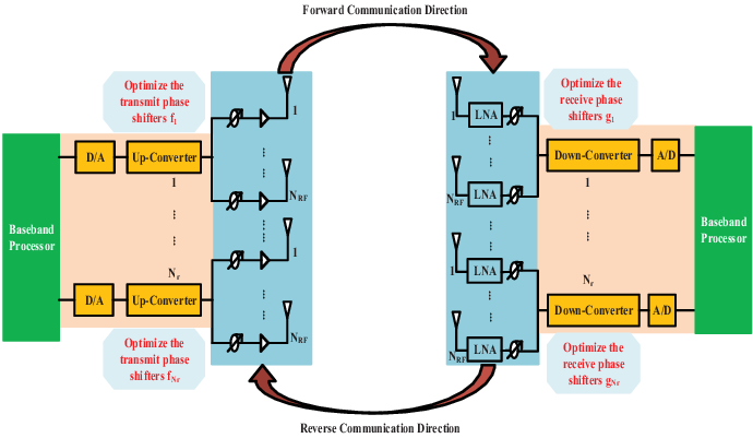
It is not difficult to find that Algorithm , Algorithm , and Algorithm can be extended to design the hybrid precoder and combiner for the multiuser MIMO interference channels with sub-connected architecture [29]. In order to show that the converge of Algorithm to Algorithm can be guaranteed, here, the total interference metric is firstly defined as
| (16) |
Proposition 1.
The sequences produced by Algorithm , Algorithm and Algorithm all are a monotonically non-increasing objective and always converge.
Proof.
For given , Algorithm aims to minimize the interference received by each receive sub-array via optimizing the receive phase shifter vector, i.e, each update of each receive sub-array phase shifter vector minimizes the objective of problem (). It also means that the iterative procedure generates a non-increasing sequence which is lower bounded by the minimum singular value of . Thus, the convergence of Algorithm is guaranteed by the monotonic boundary sequence theorem [41]. Similarly, the conclusion also holds for Algorithm . Furthermore, it is easy to see that the total interference sequence generated by Algorithm is also non-increasing sequence and the convergence of Algorithm is also guaranteed by the monotonic boundary sequence theorem [41]. ∎
III-B Digital Precoder and Combiner Optimization
Once the analog precoder and combiner are obtained, the channel coefficient between the transmitter and receiver becomes an equivalent MIMO channel and can be rewritten as
| (17) |
While the baseband received signal can be reformulated as where is the effective additive noise with zero mean and variance . Further, the spectral efficiency given by () can also be rewritten as
| (18a) | ||||
| (18b) | ||||
We apply an whitening filter at the receiver, which is shown to be related with as [51, 52]. With this whitening filter, the baseband received signal after post-processing is . Under the independence assumption of ’s and ’s, the MSE matrix can be written as
| (19) |
Combining () with (), we have . Fixing all the transmit precoder and minimizing MSE lead to the well-known MMSE receiver:
| (20) |
and
| (21) |
The corresponding MSE matrix with MMSE combiner is applied can be written as
| (22) |
From (18b) and (), it is easy to see that . Now, we resort to solve the following problem () to obtain the baseband precoder and the baseband combiner .
| (23) |
where is a positive semidefinite weight matrix and .
Note that the numerator is concave in each of the optimization variables , , and , the denominator is convex with respect to . Therefore, it belongs to the class of the standard fractional programming problem. The research results in [47, 48, 36, 37] have shown that the fractional programming problem can be transformed into a parameterized subtractive form by introducing an auxiliary variable, i.e.
| (24) |
The existing research on the fractional programming problem have shown that solving the above problem is equivalent to look up a solution of problem () such that its objective equals zero and the optimal solution of can be obtained by using Newton-like method. In what follows, we focus on solve problem () with fixed and propose to use the block coordinate descent method to solve it. Specially, we maximize the cost function by sequentially fixing two of the three variables , , and , and updating the third. It is easily known that the optimal solutions of and are respectively given by () and [53].
For fixed and , the Lagrange function of problem () is given as follows
| (25) |
where is a Lagrange multiplier associated with the power budget constraint of transmitter. The first-order optimality condition of with respect to yields
| (26) |
where and should be chosen such that the complementarity slackness condition of the power budget constraint is satisfied. Let denote the right hand of (). When the matrix is invertible and , then , otherwise the equality must be held. Let the eigendecomposition of be , then can be equivalent to
| (27) |
where . Note that the optimum (denoted by ) must be positive in this case and the left-hand side of () is a decreasing function in for and . Hence, () can be easily solved using one dimensional search techniques, such as bisection method. Plugging , the optimal can be obtained.
Thus, a two layer algorithm used to design the digital precoder and the digital combiner is summarized as Algorithm to solve problem () where is a stop threshold and denotes the objective of problem (). At the outer layer of Algorithm , the auxiliary variable is optimized via the fractional programming method [39, 40]. At the inner layer of Algorithm , due to that the cost function of () is convex in each of the optimization variables , , and , we propose to use the block coordinate descent method to solve () via alternative iteration method. In other words, () is optimized sequentially via fixing two of the three variables , , and , and updating the third.
Note that Algorithm aims to optimize the system energy efficiency and can be used to optimize the spectral efficiency by omitting the outer loop. Furthermore, Algorithm can also be applied to optimize the digital precoder and combiner without the phase shifter constraints. According to the monotonic boundary theorem and fractional programming theory, it is easy to prove the following proposition [39, 40, 41]. The computational complexity analysis is similar with that of the developed algorithms in [36, 37].
Proposition 2.
The sequence produced by Algorithm is a monotonically non-decreasing objective and always converge.
Proof.
Based on the aforementioned design method of the hybrid precoder and combiner, we can obtain a solution to problem () via alternative optimization method. First, the RF precoder and the RF combiner are designed using Algorithm aiming to minimize the total interference. Then, the baseband precoder and the baseband combiner are designed using Algorithm aiming to maximize the system energy efficiency.
IV Numerical Results
In this paper, we adopt a narrowband clustered channel representation in [26]. It is based on the extended Saleh-Valenzuela model [46] which has been used for modeling a 60-GHz wireless local area network [19] and personal area network [13]. This model allows us to accurately capture the mathematical structure presented in mmWave channels. The channel matrix is assumed to be a sum of the contributions of scattering clusters, each of which contribute propagation paths to . Therefore, the can be written as
| (28) |
where is the complex gain of the th ray in the th scattering cluster and is complex Gaussian random variable with zero mean and variance , whereas and are its azimuth (elevation) angles of arrival and departure (AoA and AoD), respectively. The mean angle associated with each cluster is uniformly distributed over , and the distribution of the difference between an AoA (AoD) and its mean is Laplacian with angular standard deviation [14, 15, 16]. The vector and are the normalized receive and transmit array response vectors at an azimuth (elevation) angle of and , respectively [26, 27, 29, 30, 31].
In our simulations, the propagation environment is model as a cluster environment with rays per cluster with Laplacian distributed azimuth and elevation angles of arrival and departure [14, 15]. For simplicity of exposition, The inter-element spacing is assumed to be half wavelength. We compare the performance of the proposed strategy to optimal unconstrained precoding in which a complete antenna array with one RF chain per antenna and the power consumption is
| (29a) | ||||
| (29b) | ||||
| (29c) | ||||
In our simulations, we set mW, mW, mW, mW and mW [54, 55, 56]. For simpicity, the value of the inefficiency of the power amplifier is set to be unit. We assume uniform linear arrays with antenna spacing of . dBm. The variance of the channel gains , and the angular standard deviation (angular spread) [26, 27, 29, 30, 31].
Fig. , Fig. , and Fig. show the convergence trajectory of Algorithm , Algorithm , and Algorithm for four random channel realizations, respectively. It is illustrated from these figures that the three algorithms converge to a stationary point within iterations. In other words, the proposed algorithms have a fast convergence speed.
flushleft
\onelinecaptionstrue
flushleft
\onelinecaptionstrue
flushleft
\onelinecaptionstrue
Fig. shows the convergence behavior of Algorithm under different allowable transmit power constraint for four random channel realizations. Numerical results also show that Algorithm can converge to a stationary point within iterations.
flushleft \onelinecaptionstrue


Fig. and Fig. show the average energy efficiency performance of proposed hybrid precoder and combiner scheme compared with digital precoder and combiner scheme under different antenna configurations and different power consumptions of over random channel realizations. Numerical results show that the digital precoder as well as combiner scheme outperforms the hybrid precoder and combiner scheme with RF chains. In other words, digital precoder and combiner scheme achieves better energy efficiency performance at the cost of higher hardware implementation and more computational complexity and channel estimation and feedback overheads. We can observe that at lower transmit power region, the hybrid precoder and combiner scheme outperforms the digital precoder and combiner schemes in the case of larger number of antennas and larger value of .
flushleft \onelinecaptionstrue


flushleft \onelinecaptionstrue


V Conclusions
In this paper, we investigated the energy efficient design of the hybrid precoder and combiner with sub-connected architecture. A two layer optimization method was presented to solve the problem of interest. First, the analog precoder and combiner were optimized via the ADOM where the phase shifter can be easily adjusted with an analytical structure. Then, the digital precoder and combiner was optimized for an effective MIMO communication systems. The convergence of the proposed algorithms were proven by using the monotonic boundary theorem and fractional programming theory. Extensive simulation results were given to validate the effectiveness of the developed method and evaluate the energy efficiency performance under various circuit power consumption model and system configuration.
References
- [1] A. Ghosh, R. Ratasuk, B. Mondal, N. Mangalvedhe, and T. Thomas, “LTE-Advanced: Next-generation wireless broadband technology,” IEEE Wireless Commun., pp. 10-22, Jun. 2010.
- [2] A. Damnjanovic, J. Montojo, Y. Wei, T. Ji, T. Luo, M. Vajapeyam, T. Yoo, O. Song, and D. Malladi, “A survey on 3GPP heterogeneous networks,” IEEE Wireless Commun., pp. 10-21, Jun. 2011.
- [3] T. Gou and S. A. Jafar, “Degrees of freedom of the user MIMO interference channel,” IEEE Trans. Inf. Theory, vol. 56, no. 12, pp. 6040-6057, Dec. 2010.
- [4] K. Gomadam, V. Cadambe, and S. Jafar, “A distributed numerical approach to interference alignment and applications to wireless interference networks,” IEEE Trans. Inf. Theory, vol. 57, no. 6, pp. 3309-3322, Jun. 2011.
- [5] S. Bi, C. Ho, and R. Zhang, “Wireless powered communication: Opportunities and challenges,” IEEE Wireless Commun., pp. 117-125, Apr. 2015.
- [6] A. Pyattaev, K. Johnsson, S. Aandreev, and Y. Koucheryavy, “Communication challenges in high-density deployments of wearable wireless devices,” IEEE Wireless Commun., pp. 12-18, Feb. 2015.
- [7] J. Andrews, S. Buzzi, W. Choi, S. Hanly, A. Lozano,A. Soong, and J. Charlie Zhang, “What will 5G be?” IEEE J. Sel. Areas Commun., vol. 32, no. 6, pp. 1065-1081, Jun. 2014.
- [8] Z. Pi and F. Khan, “An introduction to millimeter-wave mobile broadband systems,” IEEE Commun. Mag., pp. 101-107, Jun. 2011.
- [9] T. Rappaport et al., “Millimeter wave Mobile communications for 5G cellular: It will work!,” IEEE Access, vol. 1, pp. 335-349, May 2013.
- [10] W. Roh, J. Seol, J. Park, B. Lee, J. Lee, Y. Kim, J. Cho, K. Cheun, and F. Aryanfar, “Millimeter-wave beamforming as an enabling technology for 5G cellular communications: Theoretical feasibility and prototype results,” IEEE Commun. Mag., pp. 106-113, Feb. 2014.
- [11] S. Rangan, T. Rappaport, and E. Erkip, “Millimeter-wave cellular wireless networks: Potentials and challenges,” Proceedings of the IEEE, vol. 102, no. 3, pp. 366-385, Mar. 2014.
- [12] S. Han, C. Lin I, Z. Xu, and C. Rowell, “Large-scale antenna systems with hybrid analog and digital beamforming for millimeter wave 5G,” IEEE Commun. Mag., pp. 186-194, Jan. 2015.
- [13] S. Yong, “TG3c channel modeling sub-committee final report,” IEEE doc. 15-07-0584-01-003c. [Online]. Available: https://mentor.ieee.org/802.15/documents.
- [14] A. Forenza, D. Love, and R. W. Heath, Jr., “Simplified spatial correlation models for clustered MIMO channels with different array configurations,” IEEE Trans. Veh. Technol., vol. 56, no. 4, pp. 1924-1934, Jul. 2007.
- [15] H. Xu, V. Kukshya, and T. Rappaport, “Spatial and temporal characteristics of 60-GHz indoor channels,” IEEE J. Sel. Areas Commun., vol. 20, no. 3, pp. 620-630, Apr. 2002.
- [16] S. Singh, R. Mudumbai, and U. Madhow, “Interference analysis for highly directional 60-GHz mesh networks: the case for rethinking medium access control,” IEEE/ACM Trans. Netw., vol. 19, no. 5, pp. 1513-1527, Oct. 2011.
- [17] P. Chang, S. Su, S. Hsu, W. Cho, and J. Jin, “An ultra-low-power transformer-feedback P60 GHz low-noise amplifier in 90 nm CMOS?” IEEE Microw. Compon. Lett., vol. 22, no. 4, pp. 197-199, 2012.
- [18] H. Hong, H. Kang, D. Jo, D. Lee, Y. You, Y. Lee, H. Park, and S. Ryu, “26.7 A 2.6b/cycle-architecture-based 10b 1JGS/s 15.4mW 4-time-interleaved SAR ADC with a multistep hardware-retirement technique?” in Solid- State Circuits Conference - (ISSCC), 2015 IEEE International, pp. 1-3, Feb 2015.
- [19] A. Maltsev et al., “Channel Models for 60 GHz WLAN Systems,” IEEE doc. 11-09-0334-08-00ad. [Online]. Available: https://mentor.ieee.org/802.11/documents.
- [20] IEEE 802.11ad, “IEEE 802.11ad standard-Enhancements for very high throughput in the 60 GHz Band.” IEEE Computer Society.
- [21] A. Molisch and X. Zhang, “FFT-based hybrid antenna selection schemes for spatially correlated MIMO channels,” IEEE Commun. Lett., vol. 8, no. 1, pp. 36-38, Jan. 2004.
- [22] J. Wang, Z. Lan, and C. Pyo, “Beam codebook based beamforming protocol for multi-Gbps millimeter-wave WPAN systems,” IEEE J. Sel. Areas Commun., vol. 27, no. 8, pp. 1390-1399, Oct. 2009.
- [23] K. Haneda, C. Gustafson, and S. Wyne, “60 GHz spatial radio transmission: Multiplexing or Beamforming?” IEEE Trans. Antennas and Prop., vol. 61, no. 11, pp. 5735-5743, Nov. 2013
- [24] X. Zhang, A. F. Molisch, and S. Y. Kung, “Variable-phase-shift-based RF baseband codesign for MIMO antenna selection,” IEEE Trans. Signal Process., vol. 53, no. 11, pp. 4091-4103, Nov. 2005.
- [25] Z. Xiao, X. Xia, D. Jin, and N. Ge, “Iterative eigenvalue decomposition and multipath-grouping Tx/Rx joint beamformings for millimeter-wave communications,” IEEE Trans. Wireless Commun., vol. 14, no. 3, pp. 1595-1607, Mar. 2015.
- [26] O. Ayach, S. Rajagopal, S. Abu-Surra, Z. Pi, and R. Heath, Jr., “Spatially sparse precoding in millimeter wave MIMO systems,” IEEE Trans. Wireless Commun., vol. 13, no. 3, pp. 1499-1513, Mar. 2014.
- [27] A. Alkhateeb, O. E. Ayach, G. Leus, and R. W. Heath Jr., “Channel estimation and hybrid precoding for millimeter wave cellular systems,” IEEE J. Sel. Topics Signal Process., vol. 8, no. 5, pp. 831-846, Oct. 2014.
- [28] L. Liang, W. Xu, and X. Dong, “Low-complexity hybrid precoding in massive multiuser MIMO systems,” IEEE Commun. Letter, vol. 3, no. 6, pp. 653-656, Dec. 2014.
- [29] A. Alkhateeb, G. Leus, and R. Heath, Jr., “Limited feedback hybrid precoding for multi-user millimeter wave systems,” IEEE Trans. Wireless Commun., vol. 14, no. 11, pp. 6481-6494, Nov. 2015.
- [30] Y. Lee, C. Wang, and Y. Huang, “A hybrid RF/baseband precoding processor based on parallel-index-selection matrix-inversion-bypass simultaneous orthogonal matching pursuit for millimeter wave MIMO systems,” IEEE Trans. Signal Process., vol. 63, no. 2, pp. 305-317, Jan 2015.
- [31] M. Kim, and Y. Lee, “MSE-Based hybrid RF/Baseband processing for millimeter-wave communication systems in MIMO interference channels,” IEEE Trans. Veh. Tech., vol. 64, no. 6, pp. 2714-2720, Jun. 2015.
- [32] J. Zhu, Wei Xu, Ning Wang, “Secure massive MIMO systems with limited RF chains,” ,” IEEE Trans. Veh. Tech., accepted, Oct. 2016.
- [33] Y. Li, M. Daneshmand, C. Wang, and W. Zhao, “Energy Efficient Femtocell Networks: Challenges and Opportunities,” IEEE Wireless Commun., vol. 20, issue. 6, pp. 99 - 105, Dec. 2013.
- [34] Y. Li, C. Liao, Y. Wang, and C. Wang, “Energy-efficient optimal relay selection in cooperative cellular networks based on double auction,” IEEE Wireless Commun., vol. 14, no. 8, pp. 4093-4104, Aug. 2015.
- [35] Y. Li, X. Zhu, C. Liao, C. Wang, and B. Cao, “Energy efficiency maximization by jointly optimizing the positions and serving range of relay stations in cellular networks,” IEEE Trans. Veh. Technol., vol. 64, no. 6, pp. 2551-2560, Jun. 2015.
- [36] S. He, Y. Huang, S. Jin, and L. Yang, “Coordinated beamforming for energy efficient transmission in multicell multiuser systems,” IEEE Trans. Commun., vol. 61, no. 12, pp. 4961-4971, Dec. 2013.
- [37] S. He, Y. Huang, L. Yang , and B. Ottersten, “Coordinated multicell multiuser precoding for maximizing weighted sum energy efficiency,” IEEE Trans. Sig. Proc., vol. 62, no. 3, pp. 741-751, Feb. 2014.
- [38] P. Amadori and C. Masouros, “Low RF-complexity millimeter-wave beamspace-MIMO systems by beam selection,” IEEE Trans. Commun., vol. 63, no. 6, pp. 2212-2222, Jun. 2015.
- [39] R. Jagannathan, “On some properties of programming problems in parametric form pertaining to fractional programming,” Management Science, vol. 12, no. 7, pp. 609-615, Mar. 1966.
- [40] W. Dinkelbach, “On nonlinear fractional programming,” Bulletin of the Australian Mathematical Society, vol. 13, pp. 492-498, Mar. 1967.
- [41] J. Bibby, “Axiomatisations of the average and a further generalisation of monotonic sequences,” Glasgow Mathematical Journal, vol. 15, pp. 63-65, 1974.
- [42] E. Firouzjaei, mm-Wave phase shifters and switches, Electrical Engineering and computer Sciences University of California at Berkeley, Technical Report No. UCB/EECS-2010-163, December 16, 2010, http://digitalassets.lib.berkeley.edu/techreports/ucb/text/EECS-2010-163.pdf.
- [43] A. Goldsmith, S. Jafar, N. Jindal, and S. Vishwanath, “Capacity limits of MIMO channels,” IEEE J. Sel. Areas Commun., vol. 21, no. 5, pp. 684-702, 2003.
- [44] D. Tse, and P. Viswanath, Fundamentals of Wireless Communication, 1st edition. Cambridge University Press, 2005.
- [45] D. Ng, E. Lo, and R. Schober, “Energy-efficient resource allocation in OFDMA systems with large numbers of base station antennas,” IEEE Trans. Wireless Commun., vol. 11, no. 9, pp. 3292-3304, Sep. 2012.
- [46] B. Clerckx and C. Oestges, MIMO Wireless Networks, 2nd ed. New York, NY, USA: Academic, 2013.
- [47] D. Palomar, J. Cioffi, and M. Lagunas, “Joint Tx-Rx beamforming design for multicarrier MIMO channels: A unified framework for convex optimization,” IEEE Trans. Signal Process., vol. 51, no. 9, pp. 2381-2401, Sep. 2003.
- [48] D. Palomar and M. Chiang, “A tutorial on decomposition methods for network utility maximization,” IEEE J. Sel. Areas Commun., vol. 24, no. 8, pp. 1439-1451, Aug. 2006.
- [49] S. Mohammed and E. Larsson, “Single-user beamforming in large-scale MISO systems with per-antenna constant-envelope constraints: The doughnut channel,” IEEE Trans. Wireless Commun., vol. 11, no. 11, pp. 3992-4005, Nov. 2012.
- [50] N. Kumar and A. Sappal, “Coordinate rotation digital computer algorithm: Design and architectures,” (IJACSA) International Journal of Advanced Computer Science and Applications, vol. 2, no. 4, 2011.
- [51] S. Shim, J. S. Kwak, R. W. Heath, Jr., and J. G. Andrews, “Block diagonalization for multi-user MIMO with other-cell interference,” IEEE Trans. Wireless Commun., vol. 7, no. 7, pp. 2671-2681, July 2008.
- [52] D. Palomar and S. Verdu, “Gradient of mutual information in linear vector gaussian channels,” IEEE Trans. Inform. Theory, vol. 52, no. 1, pp. 141-154, Jan. 2006.
- [53] S. Christensen, R. Argawal, E. Carvalho, and J. Cioffi, “Weighted sum-rate maximization using weighted MMSE for MIMO-BC beamforming design,” IEEE Trans. Wireless Commun., vol. 7, no. 12, pp. 1-7, Dec. 2008.
- [54] S. Rangan, T. Rappaport, E. Erki, Z. Latinovic, M. R. Akdeniz, and Y. Liu, “Energy efficient methods for millimeter wave picocellular systems,” in IEEE Communication Theory Workshop, 2013.
- [55] Y. Yu, P. Baltus, A. De Graauw, E. Van Der Heijden, C. Vaucher, and A. Van Roermund, “A 60 GHz phase shifter integrated with LNA and PA in 65 nm CMOS for phased array systems,” IEEE Journal of Solid-State Circuits, vol. 45, no. 9, pp. 1697-1709, Sep. 2010.
- [56] W. Li, Y. Chiang, J. Tsai, H. Yang, J. Cheng, and T. Huang, “60-GHz 5-bit phase shifter with integrated VGA phase-error compensation,” IEEE Transactions on Microwave Theory and Techniques, vol. 61, no. 3, pp. 1224-1235, Mar. 2013.