A Probabilistic View of Neighborhood-based Recommendation Methods
Abstract
Probabilistic graphic model is an elegant framework to compactly present complex real-world observations by modeling uncertainty and logical flow (conditionally independent factors). In this paper, we present a probabilistic framework of neighborhood-based recommendation methods (PNBM) in which similarity is regarded as an unobserved factor. Thus, PNBM leads the estimation of user preference to maximizing a posterior over similarity. We further introduce a novel multi-layer similarity descriptor which models and learns the joint influence of various features under PNBM, and name the new framework MPNBM. Empirical results on real-world datasets show that MPNBM allows very accurate estimation of user preferences.
I Introduction
Collaborative filtering, which leverages user history information to predict users’ unknown preference, is one of the most successful techniques to build recommender systems [17]. Matrix factorization (MF) [12] and neighborhood-based methods (NBMs) [9] are two representative approaches. MF family attracts more attention due to its ability of modeling influence of various features (e.g. [22, 20, 11]), thus to improve accuracy. However, it is difficult to provide explainable recommendation results. NBM family, shown as Fig. 1, is very popular mainly due to the fact that it naturally explains recommendation results (e.g. An item which is similar with what you bought before). Similarity serves as the basis of weighting neighbors which is crucial to the accuracy of NBM recommender systems. However, existing similarity computation scheme is incapable of capturing influence from different features which hampers further polishing similarity to improve accuracy. In this paper, we first present a basic probabilistic framework of NBM family (PNBM) which leads learning similarity to a regression problem. Then we introduce a novel multi-layer similarity descriptor which models and learns the joint influence of different features under PNBM.
I-A Related Work
Commonly, NBMs are divided into two classes [9]. One is user-based approach which predicts the rating that a user will assign to an unrated item by referring to other users who are similar to this user. The other is item-based approach which estimates a user’s preference to an unrated item based on other items that are similar to this unrated item. The two approaches follow the same principle.
With respect to NBM, researches have mainly focused on similarity computation schemes [9] and neighbor selection strategies [5]. Similarity also serves as the basis for neighbor selection, thus we concentrate upon similarity in this paper. Generally, there are two main approaches to compute similarity. One introduces different kinds of correlation coefficients as similarity [9], such as Pearson and Cosine correlations. However, some researchers argue that such kind of methods isolate the relations between two items without leveraging global information. The other approach learns similarity via regression models. [7, 18] introduce a way to learn similarity by minimizing mean squared error between observed ratings and their corresponding estimation. [18] factors similarity matrix via low-rank approximations. [6] presents a weighted error function which gives more weight to the users who rated items most similar to the estimated item. [14, 15] simplify standard neighborhood-based models to a simple linear regression problem for top- recommendation based on binary databases.

A number of probabilistic models have been introduced to collaborative filtering. However, only a very small portion of them are NBM related. [15] presents a generic Bayesian personalized ranking framework which is optimized for the area under ROC (AUC) metric. [21] introduces a probabilistic memory-based collaborative filtering method in which they use a mixture Gaussian model built on the basis of a set of user profiles and use the posterior distribution of user ratings for prediction. [8] builds a Markov network using Pearson-correlation NBM as basis. People also place probabilistic prior assumptions to observations to model uncertainty. Such as, [10] places Dirichlet distribution on the absolute value of rating difference. [5] uses different probabilistic density functions to sample neighbors from a predefined similarity matrix (vectors).
Unfortunately, these models are incapable of representing complex features, and none of them discusses NBM family itself from a Bayesian perspective.
I-B Contribution
In this paper, we present a probabilistic (Bayesian) framework of NBM family, and our contribution is twofold.
- •
First, we present a general graphical model of NBM family (PNBM) which leads the estimation of user preference to maximizing a posterior over similarity.
- •
Then, we introduce a novel multi-layer similarity descriptor which is capable of modeling and learning the joint influence of various features (e.g. rating, text, genre) under PNBM, and we name the new framework as MPNBM.
MPNBM is evaluated on three popular real-world datasets via root-mean-square-error (RMSE) metric. Empirical results show that MPNBM consistently outperform state-of-art approaches on the datasets we choose.
II Preliminary
Suppose we have a data set organized in form of matrix , it contains users and items. is item similarity matrix, denotes similarity between item and , we further assume . presents indicator matrix, and . if user rated item , otherwise . denotes all the observed ratings.
So far, many neighborhood-based methods have been proposed, as surveyed in [9]. For simplicity, we take a variant of mean-centering NBM [16] as instance throughout the paper. The predication formula is defined in Equation (1).
| (1) |
where is rating score that user gave to item . denotes the estimation of user ’s preference on item . is the mean value of all the ratings given to item . presents a set containing all the items.
For further simplicity, Equation (1) is transformed into a vectorization form:
| (2) |
where and . denotes similarity vector corresponding to item and represents rating vector of user . The multiplication denotes the inner product of the two vectors. is an indicator vector of user . The symbol means a vector that does not contain an item which is being predicted. For example, with regard to Equation (2), denotes a vector does not contain . Moreover, we assume the testing set is excluded from the training set, when we predict in the testing set, in the training set is always zero.
III Probabilistic Framework of NBM

In this section, we present a probabilistic graphical model of NBMs (PNBM), shown in Fig. 2. It is a Bayesian network which describes the following factorization:
| (3) |
In our context, placing prior distribution on hyper-parameters does not significantly improve accuracy while dramatically increasing time complexity. For the sake of simplicity and reduction of time complexity, we simply let be constant, and is also constant. So we can simplify Equation (3) to
| (4) |
We introduce a general Gaussian distribution (but not limited to, other distribution can be also applied to. It depends on real-world context.) to density function which naturally leads to a sum-of-square-error.
More specifically, assume that an item’s similarity vector is independent from those of other items, and is sampled from a mean-zero spherical Gaussian distribution. Thus we have
| (5) |
where denotes the Gaussian distribution for with mean and precision . We also assume that ratings are independent with each other. Combine with Equation (2), we have following
| (6) |
IV Multi-layer Similarity Descriptor
In Section III, we introduced a general probabilistic (Bayesian) NBM framework which is simple and straightforward. However, like other similarity computation methods, PNBM falls short in feature representation which extremely limits the accuracy improvement. In this section, we present a multi-layer similarity descriptor (MLSD, shown in Fig.3 ) which is able to model and learn the joint influence of various features (e.g. ratings, text, genre, time). MLSD is mathematically defined as

| (7) |
where denotes the similarity basis at -th layer. is ’s constraint matrix which presents an influence of observed features. For example, it can present the similarity of text description ( or time closeness ) between any two-item. Note that different influences may be generated from the same feature. denotes the importance of the feature-influence modeled at layer . is the number of layers (influence) employed to model similarity. In this paper, we don’t require , since we always have a normalization factor in the prediction equation, i.e. Equation (2). denotes point-wise product operation (Hadamard product) on matrices and , e.g.
MLSD can be smoothly integrated into PNBM, shown in Fig. 4, named MPNBM. The Bayesian network is mathematically describe as
| (8) |
where . Follow the same assumptions in Section III, we define the prior of layer ( ) as
| (9) |
And we have the conditional distribution over observed ratings defined as
| (10) |

V Maximum a Posterior
PNBM is a specific case of MPNBM, which only has one layer with constraint-matrix set to 1. In this section, we take MPNBM as example to present how we optimize similarity via maximizing a posterior.
The log of Bayesian network defined in Equation (8) is given by
| (11) |
In fact, it defines the posterior distribution over similarity. Combine it with Equation (9) and Equation (10), we have
| (12) |
Maximizing the above Bayesian network distribution with hyper-parameters being kept fixed is equivalent to minimizing an error function defined as
| (13) |
where is the regularization parameter for layer .
A simple linear Gaussian model sometimes makes prediction value fall out of the range of valid rating values. In order to force the predication values to fall into valid range, we pass the linear-Gaussian model through hyperbolic tangent function which makes prediction values be in range of [-1,1]. We map the centralized ratings to range [-1, 1] with Equation (14).
| (14) |
where and are the max and min value of ratings, respectively. Since the ratings are centralized by their corresponding mean value, we always have and . As a result, the range of valid rating value align with the estimation produced by our models.
The conditional distribution of observed ratings becomes
| (15) |
We adopt stochastic gradient descent (SGD) as learning algorithm to train latent factors, shown in Algorithm 1.
VI Experiments
VI-A Description of Data Sets
In the experiments, we evaluate our models and state-of-art methods over three different data sets, summarized in Table I.
| data set | user# | item# | ratings# | scales | density |
| ML-20M | 138,493 | 26,744 | 20,000,263 | [0.5,5] | 0.54% |
| ML-10M | 69,878 | 1,0677 | 10,000,054 | [0.5,5] | 1.34% |
| Netflix | 32,682 | 13,139 | 3,967,477 | [1,5] | 0.92% |
| Yahoo-R4 | 7,637 | 3,791 | 207,854 | [1,5] | 0.72% |
ML-20M, ML-10M are data sets provided by MovieLens [1]. Netflix is a subset sampled from Netflix Prize data set [2] such that each user rated 50-1500 movies, and each movie is rated by 5-1800 users. Yahoo-R4 is a subset of the movie-rating data set provided by the Yahoo Labs Webscope Team [4] such that each movie are at least rated by 5 users.
- •
We use ML-10M, Netflix and Yahoo-R4 to compare the models’ accuracy.
- •
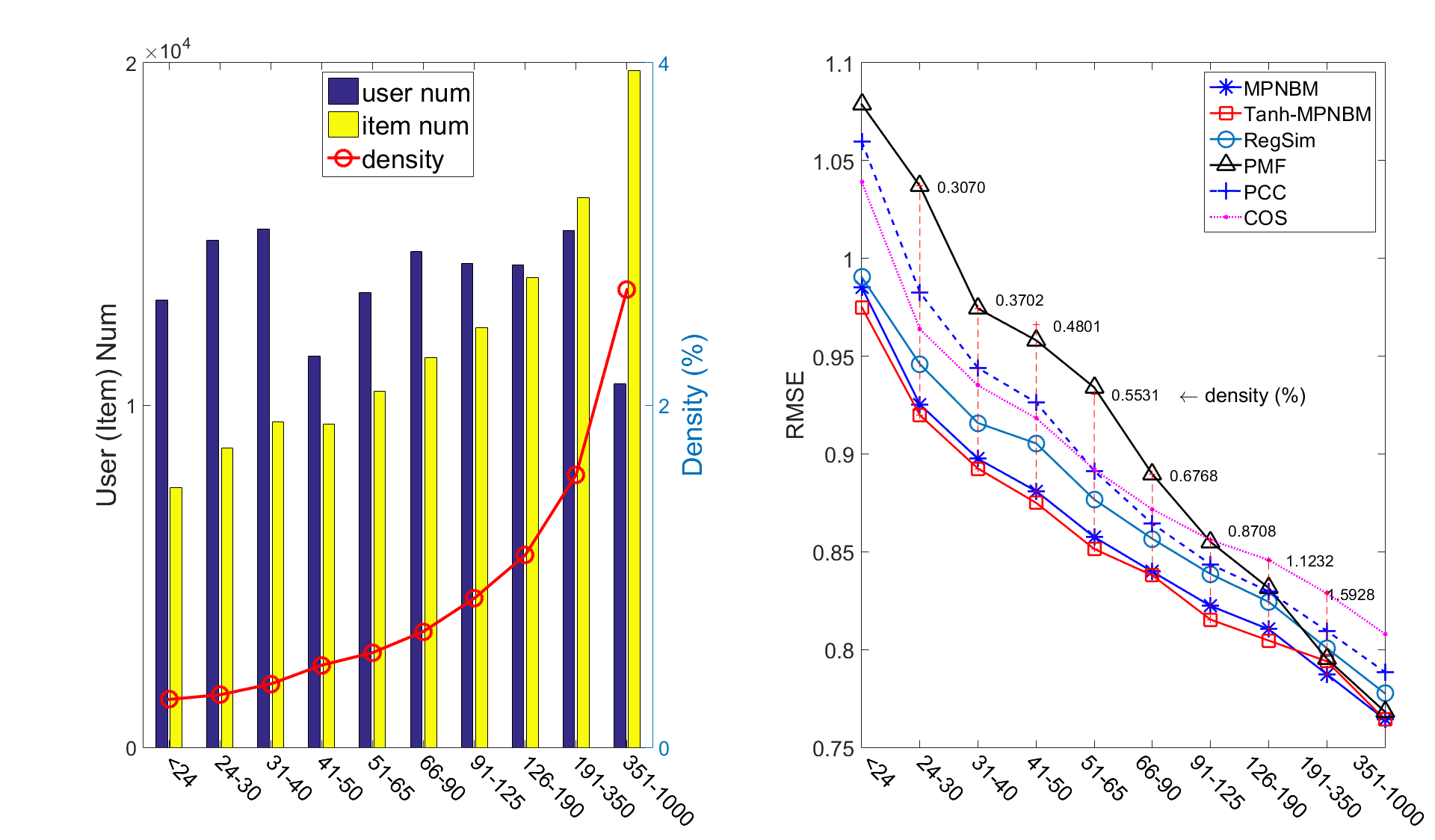
We also compare each model’s accuracy on data sets with different densities. In order to avoid the inherent differences of data sets from different originations, we extract 10 subsets from one single data set (ML-20M) based on the users’ rating number. Precisely, each subset has similar amount of users and items, the number of users and items are in range [10000, 15000] and [8000, 20000] respectively. The density of each data set is from 0.28% to 2.67%.

VI-B Models for Comparison
In this paper, the following models are compared:
- •
RegSim: Regression on similarity [18], a representative work which learns similarity via a regression method.
- •
SLIM: Sparse linear methods [14], a regression model for top- recommendation on binary data set. We extend it to a arbitrary real-value prediction model by placing a jointly Gaussian-Laplace prior on similarity vectors. It has a very similar error function as SLIM,
(16) where is a non-zero mean value of the Gaussian prior.
- •
PCC: NBM using Pearson correlation as similarity [16].
- •
COS: NBM using Cosine correlation as similarity [9].
- •
PMF: Probabilistic matrix factorization [3].
- •
MPNBM: In this paper, we exploit influence from ratings as an instance to demonstrate MLSD’s ability of modeling various features, thus to improve accuracy. We use a 3-layer similarity descriptor in which layer-1 treats latent influence equally with constraint-matrix set to 1; Layer-2 adopts Pearson correlation as constraint-matrix that stresses the influence from those items which either have significant positive correlation or strong negative correlation with the item under predication; Layer-3 employs Jaccard index to form a constraint-matrix that amplifies the influence from those items which have similar rating history, alleviates the divergence from infrequent-rated items and frequent-rated items. Time Complexity. The computational time is mainly taken by updating similarity. At a single epoch, approximately similarities are updated, where is the size of training set, is the average rating number per users and is the number of influence layers. Intuitively, a single epoch takes about 4, 260, 340 seconds on Yahoo-R4, Netflix, ML-10M respectively.
- •
Tanh-MPNBM: The model which we pass MPNBM through hyperbolic tangent function ( detailed in Section V ).
Experiment setting. All models are implemented with Matlab, and run on a single core of a Intel (R) Xeon(R) 3.50 GHz machine with 16 GB memory.
VI-C Parameters Setting
For RegSim, MPNBM, Tanh-MPNBM and SLIM, we empirically choose parameters for each model after a grid search in which . The finally chosen parameters are summarized in Table II ( indicates a model does not have such a parameter).
| RegSim | 0.1 | (0.01,,) | (,,) |
|---|---|---|---|
| MPNBM | 0.2 | (0.05,0.05,0.05) | (3,1,1) |
| Tanh-MPNBM | 0.4 | (0.05,0.05,0.05) | (3,1,1) |
| SLIM | 0.4 | (0.02,,) | (,,) |
For PMF, we choose latent feature dimension and the momentum of mini-batch SGD . Regularized parameters ( for user latent factors and latent item factors respectively) and learning rate are set to
For PCC and COS, we use top-200 the most similar neighbors for prediction.
VI-D Comparison Results
During the test, we randomly divide each data set into training set (85%), validation set (5%) and testing set (10%). We adopt RMSE for evaluation. We repeat the experiments 5 times.
| Yahoo-R4 | Netflix | ML-10M | ||||
|---|---|---|---|---|---|---|
| RMSE | INC% | RMSE | INC% | RMSE | INC% | |
| RegSim | 0.9723 | 0 | 0.8713 | 0 | 0.8034 | 0 |
| MPNB | 0.9641 | 0.84 | 0.8425 | 3.31 | 0.7941 | 1.16 |
| TMPN | 0.9629 | 0.97 | 0.8363 | 4.02 | 0.7955 | 0.98 |
| SLIM | 0.9725 | -0.02 | 0.8731 | -0.21 | 0.8004 | 0.37 |
| PMF | 1.0608 | -9.1 | 0.8826 | -1.3 | 0.7957 | 0.96 |
| PCC | 0.9813 | -0.93 | 0.8620 | 1.07 | 0.8121 | -1.08 |
| COS | 0.9722 | 0.01 | 0.8605 | 1.24 | 0.8362 | -4.08 |
VI-D1 Accuracy
The comparison is performed over :
- •
Accuracy on different data sets.
- •
Accuracy on different density.
Fig. 5 presents the detail of training on different data sets. Table III records the final accuracy comparison (the training process is conducted by validation set). RegSim is selected as baseline model, the accuracy improvement of each model is displayed in the INC % column.
Fig. 6 shows the accuracy comparison on data sets with different density. MPNBM and Tanh-MPNBM consistently outperform outperform state-of-art models, especially on those extremely sparse data sets ( which have serious cold start problem). For simplicity, we don’t draw SLIM on the graph, since SLIM has similar accuracy with RegSim.

We are also interested in that how the layer importance-factor affects the MPNBM (Tanh-MPNBM). We use two strategies to select parameters for each layer, 1) we consistently choose for all the three data sets, named TMPN-V1; 2) letting , we assign higher value to the which corresponding has lower RMSE, named TMPN-V2. The comparison is shown in Fig. 7, and 1) the accuracy is not significantly influenced, MPNBM (Tanh-MPNBM) is able to balance the influence automatically. 2) Assigning proper weight to according to the RMSE of results in faster convergence.
VI-D2 Stability
Model based approach may easily over fit when increasing the number of parameters under training. The system can be beneficent from the stability of algorithms which is defined by
- •
converge speed: the first epoch where a model converges to the local best solution, denoted as .
- •
ability of models to maintain their best status: the number of epochs that a model stays in the local best solution, denoted as .
Table IV shows the values of and of each model over different data sets.
| Yahoo-R4 | Netflix | ML-10M | ||||
|---|---|---|---|---|---|---|
| RegSim | 86 | 102 | 134 | 67 | 96 | 91 |
| MPNBM | 84 | 59 | * | 141 | 60 | |
| Tanh-MPNBM | 158 | 43 | 166 | 35 | 115 | 86 |
| SLIM | 39 | 51 | 186 | 15 | 150 | 51 |
| PMF | 87 | 6 | 64 | 12 | 93 | 34 |
In the comparison of stability, we treat RMSE values , if . Note that with regard to a model which does not over fit after 200 epochs (value of prefixed with ), if the lowest RMSE value appears at least 10 epochs, it is seen as the local best solution. * in Table IV means a model does not converge after 200 epochs on a data set. e.g, MPNBM does not converge on Netflix data set, also shown in Fig. 5. The experimental results show that MPNBM and Tanh-MPNBM stay in the local best solution for many ( 40) epochs which is better than PMF. With regard to converge speed, as shown in Table IV, it seems that sometimes MPNBM and Tanh-MPNBM do not converge as fast as PMF. In fact, they achieve a considerable accuracy at a much earlier epoch.
VII Conclusion
In this paper, we have presented a probabilistic framework of NBM family, and introduced a multi-layer similarity descriptor under PNBM which is capable of modeling and learning the joint influence of various features. Our experiments show that MPNBM and Tanh-MPNBM allow accurate and stable estimation of user preferences.
Privacy is a serious problem to recommender systems. Nowadays, applying differential privacy to recommendation algorithms attracts great attention. A common approach is adding noise to data set. Recently, people find that sampling from a posterior distribution achieves some extent of differential privacy “for free” [19], and this idea has been already successfully applied to probabilistic matrix factorization [13]. Following the same idea, our models can also provide such kind of “free privacy”. We leave a detailed investigation as future work.
VIII Acknowledgments
Both authors are supported by a CORE (junior track) grant from the National Research Fund, Luxembourg. Qiang Tang is also partially supported by an internal project from University of Luxembourg.
References
- [1] Movielens, http://grouplens.org/datasets/movielens/.
- [2] Netflix prize, https://www.netflix.com.
- [3] http://www.utstat.toronto.edu/~rsalakhu/BPMF.html.
- [4] Yahoo!: Webscope movie data set (version 1.0), http://research.yahoo.com/.
- [5] P. Adamopoulos and A. Tuzhilin. On over-specialization and concentration bias of recommendations: Probabilistic neighborhood selection in collaborative filtering systems. In Proceedings of the 8th ACM Conference on Recommender systems, pages 153–160. ACM, 2014.
- [6] R. Bell, Y. Koren, and C. Volinsky. Modeling relationships at multiple scales to improve accuracy of large recommender systems. In Proceedings of the 13th ACM SIGKDD international conference on Knowledge discovery and data mining, pages 95–104. ACM, 2007.
- [7] R. M. Bell and Y. Koren. Scalable collaborative filtering with jointly derived neighborhood interpolation weights. In Data Mining, 2007. ICDM 2007. Seventh IEEE International Conference on, pages 43–52. IEEE, 2007.
- [8] A. Defazio and T. Caetano. A graphical model formulation of collaborative filtering neighbourhood methods with fast maximum entropy training. arXiv preprint arXiv:1206.4622, 2012.
- [9] C. Desrosiers and G. Karypis. A comprehensive survey of neighborhood-based recommendation methods. In Recommender systems handbook, pages 107–144. Springer, 2011.
- [10] G. Guo, J. Zhang, and N. Yorke-Smith. A novel bayesian similarity measure for recommender systems. In Proceedings of the Twenty-Third international joint conference on Artificial Intelligence, pages 2619–2625. AAAI Press, 2013.
- [11] Y. Koren. Factorization meets the neighborhood: a multifaceted collaborative filtering model. In Proceedings of the 14th ACM SIGKDD international conference on Knowledge discovery and data mining, pages 426–434. ACM, 2008.
- [12] Y. Koren, R. Bell, and C. Volinsky. Matrix factorization techniques for recommender systems. Computer, (8):30–37, 2009.
- [13] Z. Liu, Y.-X. Wang, and A. Smola. Fast differentially private matrix factorization. In Proceedings of the 9th ACM Conference on Recommender Systems, pages 171–178. ACM, 2015.
- [14] X. Ning and G. Karypis. Slim: Sparse linear methods for top-n recommender systems. In Data Mining (ICDM), 2011 IEEE 11th International Conference on, pages 497–506. IEEE, 2011.
- [15] S. Rendle, C. Freudenthaler, Z. Gantner, and L. Schmidt-Thieme. Bpr: Bayesian personalized ranking from implicit feedback. In Proceedings of the twenty-fifth conference on uncertainty in artificial intelligence, pages 452–461. AUAI Press, 2009.
- [16] P. Resnick, N. Iacovou, M. Suchak, P. Bergstrom, and J. Riedl. Grouplens: an open architecture for collaborative filtering of netnews. In Proceedings of the 1994 ACM conference on Computer supported cooperative work, pages 175–186. ACM, 1994.
- [17] X. Su and T. M. Khoshgoftaar. A survey of collaborative filtering techniques. Advances in artificial intelligence, 2009:4, 2009.
- [18] A. Töscher, M. Jahrer, and R. Legenstein. Improved neighborhood-based algorithms for large-scale recommender systems. In Proceedings of the 2nd KDD Workshop on Large-Scale Recommender Systems and the Netflix Prize Competition, page 4. ACM, 2008.
- [19] Y.-X. Wang, S. E. Fienberg, and A. Smola. Privacy for free: Posterior sampling and stochastic gradient monte carlo. arXiv preprint arXiv:1502.07645, 2015.
- [20] J. Yang, Z. Sun, A. Bozzon, and J. Zhang. Learning hierarchical feature influence for recommendation by recursive regularization. In Proceedings of 10th ACM Conference on Recommender Systems.(RecSys 2016). ACM, 2016.
- [21] K. Yu, A. Schwaighofer, V. Tresp, X. Xu, and H.-P. Kriegel. Probabilistic memory-based collaborative filtering. Knowledge and Data Engineering, IEEE Transactions on, 16(1):56–69, 2004.
- [22] Y. Zheng, B. Mobasher, and R. Burke. Incorporating context correlation into context-aware matrix factorization. In Proceedings of the 2015 International Conference on Constraints and Preferences for Configuration and Recommendation and Intelligent Techniques for Web Personalization-Volume 1440, pages 21–27. CEUR-WS. org, 2015.