Efficient Multi-Dimensional Mapping Using QAM Constellations for BICM-ID

Hassan M. Navazi and Md. Jahangir Hossain, Member, IEEE Affiliation: The University of British Columbia, Kelowna, BC, Canada
hnavazi@alumni.ubc.ca, jahangir.hossain@ubc.ca

Abstract

Bit-interleaved coded modulation with iterative decoding (BICM-ID) offers very good error performance over additive white Gaussian noise (AWGN) and fading channels if it uses a wisely designed signal mapping. Further, error performance of BICM-ID can significantly be improved by employing multi-dimensional (MD) modulation. However, suitable MD mappings are obtained by computer search techniques except for MD modulations that use smaller constellation e.g., binary phase shift keying (BPSK), quadrature phase shift keying (QPSK) and $8$ -ary phase shift keying ( $8$ -PSK) as basic modulation. The alphabet size of MD modulations increases exponentially as the order of the basic modulation increases and computer search becomes intractable. In this paper, we propose a systematic mapping method for MD modulations. The innovativeness of our proposed method is that it generates MD mappings using $16$ - and $64$ -quadrature amplitude modulation (QAM) very efficiently. The presented numerical results show that the proposed method improves bit error rate (BER) of BICM-ID.

Index Terms:

BICM-ID, multi-dimensional signal mapping, QAM constellations.

I Introduction

In [1], Zehavi proposed bit-interleaved coded modulation (BICM) which was analytically investigated by G. Caire et al [2]. BICM uses a bit-interleaver to separate the modulator from the encoder. Due to this separation, the modulator can be chosen independently from the encoder and it increases design flexibility [2]. It also improves the time diversity order of coded modulation [1]. Although random interleaving improves performance of BICM over fading channels, it reduces the minimum Euclidean distance between signals and degrades performance over additive white Gaussian noise (AWGN) channels [3]. To overcome this problem, iterative decoding was proposed for BICM receiver [4]-[6]. The resulted system is known as BICM with iterative decoding (BICM-ID) and achieves a significant coding gain through iterations. As such a good performance is obtained over both AWGN and fading channels [7].

Symbol mapping is defined as labeling of constellation symbols with binary digits. It is well-known that the performance of BICM-ID depends on the applied symbol mapping and a number of works has been carried out to address this issue, see for examples, [7]-[21]. If a sequence of bits is mapped to a vector of symbols (symbol-vector) rather than a single symbol, the mapping is referred to as multi-dimensional (MD) mapping [11]. For example, if $N$ symbols from phase shift keying (PSK) or quadrature amplitude modulation (QAM) are used in each symbol-vector, a $2N$ -D modulation is obtained. In fact, error performance of BICM-ID can be significantly improved by employing MD modulation due to the increased Euclidean distance between symbol-vectors [11], [21].

Although a higher order MD modulation offers more flexibility in generating good mappings for BICM-ID [13], it tremendously increases the number of possible mappings. In particular, $2N$ -D modulations using $2^{m}$ -QAM symbols have $2^{mN}!$ possible mappings where $!$ denotes a factorial operation. So, it is difficult to find good/optimum mappings for MD modulations. This problem is more severe when MD modulations are constructed using higher order 2-D modulations. For example, the number of possible mappings for $4$ -D modulation using $16$ -QAM approaches infinity. Suitable MD mappings are obtained by computer search techniques except for MD modulations that use smaller constellation e.g., binary PSK (BPSK), quadrature PSK (QPSK) and $8$ -PSK as basic modulation. The so-called binary switch algorithm (BSA) [8] is the best known computer search method for finding good mappings. However to obtain suitable mappings for larger modulations such as MD modulations, the BSA becomes intractable due to its complexity [20]. In [20] and [22], authors demonstrated that random mapping can lead to efficient MD mappings. According to the random mapping technique, computer search is used to obtain a good mapping from a large set of randomly generated mappings that makes the procedure complex. Moreover, it degrades the resulted mappings’ performance especially for larger MD modulations.

In this paper, we propose an efficient mapping method for MD modulations that use $2^{m}$ -QAM ( $m=4,6$ ) as basic modulation. Our goal is to obtain mappings which achieve a lower error rate for BICM-ID at low SNR values as well as at high SNR values. A similar objective is considered in [10] where the authors used a doping technique (combining two mappings) to obtain mappings for $2$ -D modulations. However, instead of combining mappings, we develop a single mapping for a given MD modulation to achieve a lower error rate for BICM-ID at low SNR values as well as at high SNR values. Furthermore, our proposed method yields mappings for MD constellations rather than $2$ -D ones. The proposed method is a heuristic-based technique and does not employ any computer search. The presented numerical results show that our approach not only yields mapping efficiently but also improves bit error rate (BER) performance of BICM-ID over both AWGN and Rayleigh fading channels. For example, it can save about $3$ dB transmit signal energy for a target BER of $10^{-6}$ compared to the mappings found by the BSA and random mappings.

The rest of the paper is organized as follows. While in Section II we provide BICM-ID system model, in Section III we describe the design criteria of MD mappings for BICM-ID over AWGN and Rayleigh fading channels. In Section IV, we describe our proposed MD mapping method. In Section V, we present numerical results and compare the performance of our resulted mapping. Finally, Section VI concludes the paper.
Notations: Throughout the paper, we use a lowercase letter e.g., $x$ to represent a variable, a boldface letter e.g., $\boldsymbol{x}$ to denote a row vector, and $x^{(i)}$ to represent $i$ th element of $\boldsymbol{x}$ . The norm of a vector is denoted by $\|\boldsymbol{x}\|$ which is defined as $\|\boldsymbol{x}\|^{2}=\sum_{i=1}^{N}x_{i}^{2}$ . Blackboard bold letters $\mathbb{E}$ and $\mathbb{O}$ denote the set of even integers and the set of odd integers, respectively. All-ones vector is also represented by $\boldsymbol{1}$ .

II System Model

A BICM-ID system model is shown in Fig. 1 where a sequence of information bits ${\boldsymbol{u}}$ is encoded by a convolutional encoder. Then, the coded bits ${\boldsymbol{c}}$ are randomly interleaved and the interleaved coded bits ${\boldsymbol{v}}$ are grouped in blocks of $mN$ bits. For notational convenience, let us denote $t$ th block of interleaved coded bits at the input of the modulator by $\boldsymbol{l}_{t}=[l_{t}^{(1)},l_{t}^{(2)},\cdots,l_{t}^{(mN)}]$ . The modulator maps ${\boldsymbol{l}}_{t}$ to a vector of $N$ consecutive $2^{m}$ -ary signals, ${\boldsymbol{x}}_{t}=[x_{t}^{(1)},x_{t}^{(2)},\cdots,x_{t}^{(N)}]$ , using a MD mapping function $\mu:\{0,1\}^{mN}\longrightarrow\boldsymbol{\chi}=\chi^{N}$ where $\chi$ denotes the $2$ -D $2^{m}$ -ary signal set. Mathematically, we can write

{\boldsymbol{x}}_{t}=[x_{t}^{(1)},x_{t}^{(2)},\cdots,x_{t}^{(N)}]=\mu({\boldsymbol{l}}_{t}).

(1)

Refer to caption — Fig. 1: The block diagram of a BICM-ID system.

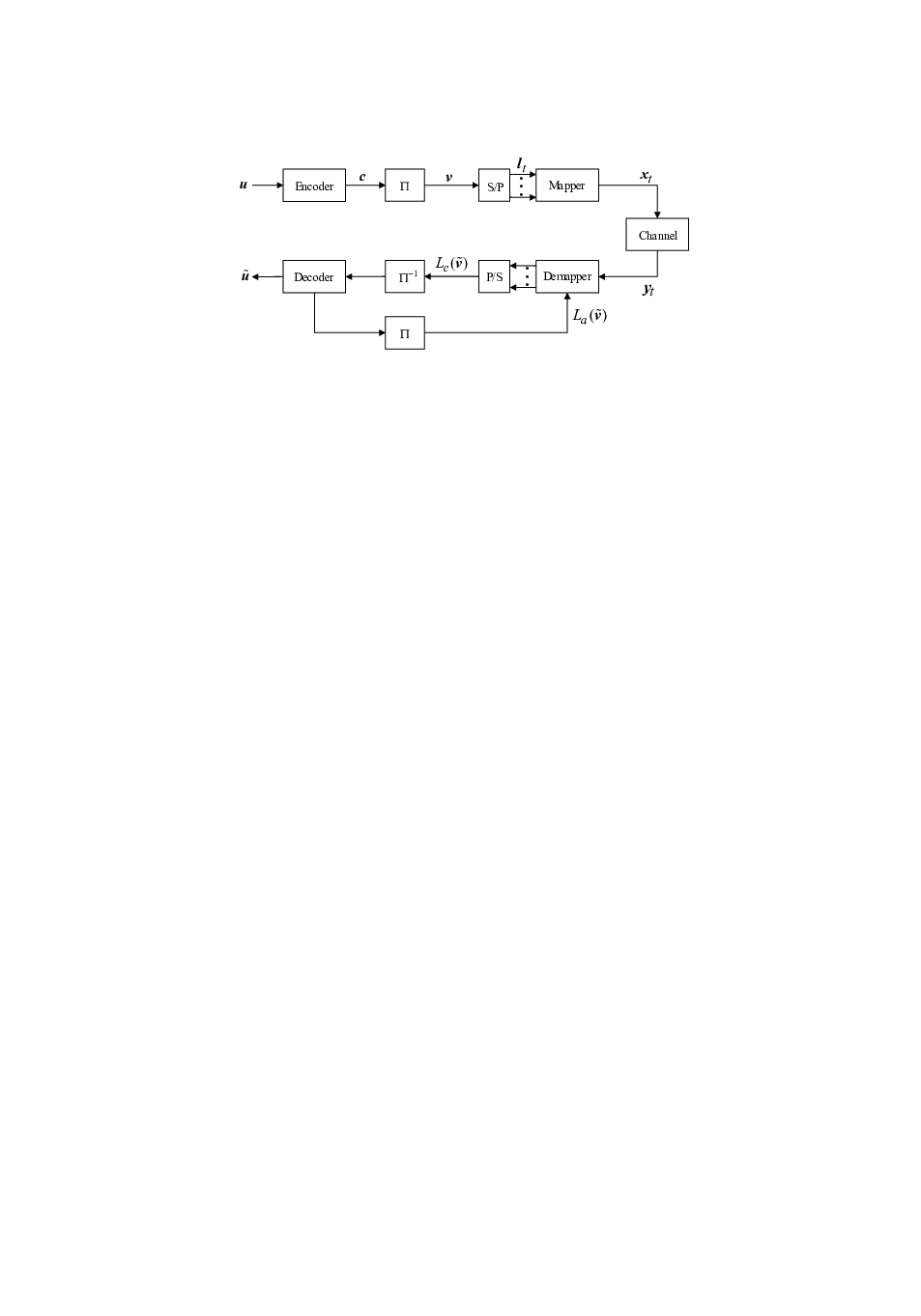
The average energy per symbol-vector is assumed to be $1$ , i.e., $E_{\boldsymbol{x}_{t}}=1$ . At the receiver, the received signal vector corresponding to the transmitted symbol-vector $\boldsymbol{x}_{t}$ can be expressed as

{\boldsymbol{y}}_{t}=\boldsymbol{h}^{T}_{t}{\boldsymbol{x}}_{t}+{\boldsymbol{n}}_{t},

(2)

where ${\boldsymbol{h}}_{t}=[h_{t}^{(1)},h_{t}^{(2)},\cdots,h_{t}^{(N)}]$ is the corresponding vector of the Rayleigh fading coefficients, $A^{T}$ represents the transpose of $A$ , and ${\boldsymbol{n}}_{t}$ is a vector of $N$ additive complex white Gaussian noise samples with zero-mean and variance $N_{0}$ . We consider two types of fading channels as follows: (i) all $N$ symbols in a symbol-vector experience a constant fading coefficient, i.e., block-fading channel [23]-[24] and (ii) the coefficients vary over the consecutive symbols in a symbol-vector, i.e., fast fading channel. Clearly, $\boldsymbol{h}_{t}=\boldsymbol{1}$ corresponds to the AWGN channel. For brevity, we omit the index $t$ in subsequent sections. It is assumed that the receiver has the perfect channel state information (CSI).

At the receiver, the demapper uses the received signal $\boldsymbol{y}_{t}$ and the a priori log-likelihood ratio (LLR) of the coded bits to compute the extrinsic LLR for each of the bits in the received symbol as described in [5]. Next, the random deinterleaver permutes the extrinsic LLRs which are used by the channel decoder. The decoder uses the BCJR algorithm [25] to calculate the extrinsic LLR values of the coded bits. These LLR values are interleaved and fed back to the demapper that uses them as the a priori LLR values in the next iteration.

III Motivation and Design Criteria of MD mappings for BICM-ID

In low SNR region, the performance of BICM-ID depends on the BER at the first iteration, i.e., BICM-ID is equivalent to BICM. So, the optimum mapping for BICM-ID in low SNR region corresponds to the optimum mapping for BICM. However, the optimal mapping designed for low SNR region is not suitable for BICM-ID in high SNR region. The reason can be explained as follows. Although the optimal mapping designed for low SNR region provides an early turbo cliff in BER performance, it offers a poor error-floor which reaches the BER range of practical interest, e.g., $10^{-6}$ at a very high SNR value. On the other hand, the mapping, which is designed to minimize the asymptotic error rate of BICM-ID, results in extremely low BER at a very high SNR value. Hence, the optimal mapping that minimizes asymptotic error rate is not very relevant for practical communication systems. Moreover, finding the optimal mapping that minimizes error-floor is computationally expensive. Therefore, designing an efficient MD mapping for BICM-ID that offers good BER in both low and high SNR regions is very desirable. Motivated by the above discussion, our objective is to develop an efficient MD mapping method for BICM-ID to achieve good BER performance over AWGN and Rayleigh fading channels in both low and high SNR regions. In what follows, we investigate the design criteria to achieve a good mapping for AWGN and Rayleigh fading channels. It is important to mention that in order to investigate the design criteria of a suitable mapping in low SNR region, we consider BICM-ID performance at the first iteration.

III-A AWGN Channel

III-A1 Low SNR region

Let ${\boldsymbol{d}}=\{d_{1},\cdots,d_{p}\}$ be the set of all possible Euclidean distances between two signal points in $\boldsymbol{\chi}$ where $d_{i}<d_{j}$ if ${i}<{j}$ and $p$ depends on the constellation. For example, $p$ takes value two and five, respectively, for 2-D and 4-D QPSK. A larger value of $d_{1}$ is desired to achieve a better BER performance of BICM over AWGN channel [2]. Moreover, in order to achieve a good asymptotic BER performance of BICM over AWGN channel, the value of $N_{min}$ should be as small as possible [2] where $N_{min}$ is defined as

N_{min}=\dfrac{1}{mN2^{mN}}\sum_{i=1}^{mN}\sum_{b=0}^{1}\sum_{{\boldsymbol{x}}\in\boldsymbol{\chi}_{b}^{i}}N({\boldsymbol{x}},i)

(3)

where $\boldsymbol{x}=(x_{1},x_{2},\cdots,x_{N})$ is a $2N$ -D signal point, $\boldsymbol{\chi}_{b}^{i}$ is the subset of all $\boldsymbol{x}\in\boldsymbol{\chi}$ whose labels take value $b$ in $i$ th bit position, and $N({\boldsymbol{x}},i)$ is the number of signal points at the Euclidian distance $d_{1}$ from ${\boldsymbol{x}}$ that are different from ${\boldsymbol{x}}$ in $i$ th bit position.

III-A2 High SNR region

$\hat{d}_{min}^{2}$ , which is defined as the minimum squared Euclidean distance (MSED) between two symbol-vectors with Hamming distance one, is the dominant factor for the asymptotic performance of BICM-ID over AWGN channels [26].

III-B Block-Fading Channel

The so called harmonic mean of the MSED [2] of mappings is a well-known parameter that relates to the BER performance of BICM-ID in Rayleigh fading channels and is defined as [2]

\Phi_{br}(\mu,\boldsymbol{\chi})=\left(\dfrac{1}{mN2^{mN}}\sum_{i=1}^{mN}\sum_{b=0}^{1}\sum_{{\boldsymbol{x}}\in\boldsymbol{\chi}_{b}^{i}}\dfrac{1}{\|{\boldsymbol{x}}-\hat{\boldsymbol{x}}\|^{2}}\right)^{-1}.

(4)

For the performance at the first iteration, $\hat{\boldsymbol{x}}$ refers to the nearest neighbor of $\boldsymbol{x}$ in $\boldsymbol{\chi}_{\bar{b}}^{i}$ and (4) is referred to as harmonic mean of the MSED before feedback. For the asymptotic performance $\boldsymbol{\chi}_{\bar{b}}^{i}$ involves only one symbol-vector $\hat{\boldsymbol{x}}$ which is different from $\boldsymbol{x}$ in only $i$ th bit position [26]. In this case, (4) is referred to as harmonic mean of the MSED after feedback which is denoted by $\hat{\Phi}_{br}(\mu,\boldsymbol{\chi})$ . To achieve a good performance at the first iteration, a larger value of $\Phi_{br}(\mu,\boldsymbol{\chi})$ is desired. Let $n_{i}$ be defined as

n_{i}=\sum_{j=1}^{mN}\sum_{b=0}^{1}\sum_{{\boldsymbol{x}}\in\boldsymbol{\chi}_{b}^{j}}I_{i}({\boldsymbol{x}},\hat{\boldsymbol{x}});~~~~~~i=1,\cdots,p,

(5)

where $I_{i}({\boldsymbol{x}},\hat{\boldsymbol{x}})$ is an indicator function that takes value one if the Euclidean distance between ${\boldsymbol{x}}$ and $\hat{\boldsymbol{x}}$ is equal to $d_{i}$ , otherwise it is equal to zero. Then, substituting (5) into (4), we obtain

\Phi_{br}(\mu,\boldsymbol{\chi})=\left(\dfrac{1}{mN2^{mN}}\sum_{i=1}^{p}\dfrac{n_{i}}{d_{i}^{2}}\right)^{-1}.

(6)

In what follows, we describe the mapping design criteria for block-fading channel in low and high SNR regions.

III-B1 Low SNR region

In low SNR region, $\hat{\boldsymbol{x}}$ in (4) is the nearest neighbour of $\boldsymbol{x}$ in $\boldsymbol{\chi}_{\bar{b}}^{i}$ . Since each signal is different from its nearest neighbor at least in one bit position, $\hat{\boldsymbol{x}}$ is at the Euclidean distance $d_{1}$ from $\boldsymbol{x}$ for some values of $i$ . As a result, $n_{1}$ in (6) has a non-zero value. Moreover, summation of $n_{i}$ for all $i$ is constant, i.e.,

\sum_{i=1}^{p}n_{i}=mN2^{mN}.

(7)

Considering (6) and (7), it is obvious that any reduction in $n_{i}$ for a specific $i$ without increasing $n_{j}$ , where $j<i$ , yields a larger value of $\Phi_{br}(\mu,\boldsymbol{\chi})$ . In particular, one can increase $\Phi_{br}(\mu,\boldsymbol{\chi})$ by decreasing $n_{1}$ .

III-B2 High SNR region

For the asymptotic performance of BICM-ID, $\hat{\boldsymbol{x}}$ is considered to be different from $\boldsymbol{x}$ only in $i$ th bit position. In other words, $\boldsymbol{\chi}_{\bar{b}}^{i}$ includes only one signal. As a result, it is possible to design a mapping in which $\hat{d}_{min}>d_{i}$ for some small values of $i$ . This gives $n_{i}=0$ for some small values of $i$ and it yields a greater value for $\hat{\Phi}_{br}(\mu,\boldsymbol{\chi})$ . Numerical examples show that a significant increase in $\hat{d}_{min}$ leads to a considerable enhancement in $\hat{\Phi}_{br}(\mu,\boldsymbol{\chi})$ .

III-C Fast Rayleigh Fading Channel

The effect of mapping on the BER performance of BICM-ID over the fast Rayleigh fading channel is characterized by $\Phi_{fr}(\mu,\boldsymbol{\chi})$ which is expressed as [27]

\Phi_{fr}(\mu,\boldsymbol{\chi})=\left(\dfrac{1}{mN2^{mN}}\sum_{i=1}^{mN}\sum_{b=0}^{1}\sum_{{\boldsymbol{x}}\in\boldsymbol{\chi}_{b}^{i}}\prod_{j=1}^{N}\left(1+\dfrac{\|{x_{j}}-\hat{x}_{j}\|^{2}}{4N_{0}}\right)^{-1}\right)^{-1}.

(8)

In particular, a greater value of $\Phi_{fr}$ offers a better BER performance for BICM-ID. Similar to the block-fading case, it is easy to show that by decreasing $n_{1}$ and increasing $\hat{d}_{min}$ one can improve $\Phi_{fr}(\mu,\boldsymbol{\chi})$ at low and high SNR values, respectively.

In summary, it can be concluded that a mapping which offers a small value of $N_{min}$ while it gives a large value of $\hat{d}_{min}$ , is suitable to achieve good error performance of BICM-ID over both AWGN and Rayleigh fading channels in low and high SNR regions. A small value of $N_{min}$ implies that the average Hamming distance between neighbouring symbols, i.e., symbols with Euclidean distance $d_{1}$ , is small and consequently $n_{1}$ is small. This eventually increases $\Phi_{br}(\mu,\boldsymbol{\chi})$ and $\Phi_{fr}(\mu,\boldsymbol{\chi})$ at the first iteration of BICM-ID in Rayleigh fading channels. So, a small value of $N_{min}$ can improve the mapping’s performance at the first iteration, i.e., in low SNR region not only in AWGN channel but also in Rayleigh fading channels. On the other hand, a large value of $\hat{d}_{min}$ implies that $n_{i}$ is equal to zero for small values of $i$ . This increases $\hat{\Phi}_{br}(\mu,\boldsymbol{\chi})$ and $\Phi_{fr}(\mu,\boldsymbol{\chi})$ at high SNR values. As a consequence, the asymptotic BER performance of BICM-ID improves over AWGN and Rayleigh fading channels as the value of $\hat{d}_{min}$ increases.

IV Proposed Mapping Method

Based on the above discussion, we take a heuristic approach to obtain a mapping that offers good BER performance in low and high SNR regions over AWGN and Rayleigh fading channels. In particular, we apply two key techniques as follows. First, to generate a mapping with a large value of $\hat{d}_{min}$ , we map binary labels with the Hamming distance one to the symbol-vectors with a large Euclidean distance. This leads to good error-floors in Rayleigh fading and AWGN channels. Second, most of the nearest neighbouring symbol-vectors are mapped to the binary labels that have Hamming distance two. This results in a small value of $N_{min}$ and yields good BER performance in low SNR region over AWGN and Rayleigh fading channels.

The proposed MD mapping using $2^{m}$ -QAM symbols is obtained progressively in $(m-1)$ steps. The mappings in steps $i~(1\leq i\leq(m-2))$ are intermediate mappings whereas the mapping in step $i=(m-1)$ is the final mapping. In $i$ th step, $2^{i+1}$ symbols from $2^{m}$ -ary constellation are selected to be used in the mapping process. The symbols selection process is descried as below.

IV-A Symbols Selection Process

We assume that position-indexes of symbols in a given QAM constellation, increase by moving right or down. For example, Fig. 2(a) shows a $16$ -QAM constellation where $S_{j}$ represents the symbol with position-index $j$ and $j$ increases from left to right or from top to bottom. The general-principles in choosing $2^{i+1}$ symbols from a $2^{m}$ -QAM constellation in $i$ th step are as follows: (i) by moving the set of selected symbols one can cover all symbols of the constellation, provided that each symbol is covered only one time. In other words, the square $M$ -QAM constellations can be partitioned into a number of subsets where the structures/shapes formed by these subsets are congruent with one another. Thus, by moving one of the subsets and superimposing it on the remaining subsets, one can cover all symbols in the constellation while each symbol is covered only once. (ii) The MSED between the chosen symbols is as large as possible. Without loss of generality, let us use ${\chi}_{i}$ to denote the set of $2^{i+1}$ chosen symbols in step $i$ and ${\boldsymbol{\alpha}}_{i}=[\alpha^{(1)}_{i},\alpha^{(2)}_{i},\cdots,\alpha^{(2^{i+1})}_{i}]$ indicates the position-indexes of symbols in ${\chi}_{i}$ . The set of used symbols in step $(i+1)$ contains all the used symbols in step $i$ , i.e., ${\chi}_{i}\subset{\chi}_{i+1}$ and ${\boldsymbol{\alpha}}_{i}\subset{\boldsymbol{\alpha}}_{i+1}$ .

Example 1

In step $i=1$ , four symbols are selected from a 16-QAM constellation to be used in the mapping process. There are four distinct sets, which are made of four symbols, as follows: $\mathcal{S}_{1,1}=\{S_{1},S_{2},S_{3},S_{4}\}$ , $\mathcal{S}_{1,2}=\{S_{1},S_{2},S_{5},S_{6}\}$ , $\mathcal{S}_{1,3}=\{S_{1},S_{3},S_{5},S_{7}\}$ , and $\mathcal{S}_{1,4}=\{S_{1},S_{3},S_{9},S_{11}\}$ . It is obvious that by moving any of these sets, one can cover all symbols of 16-QAM constellation, provided that each symbol is covered only once. Among these sets, $\mathcal{S}_{1,4}$ provides the maximum value of MSED between its symbols. As a result, for 16-QAM, we have ${\chi}_{1}=\mathcal{S}_{1,4}$ and $\boldsymbol{\alpha}_{1}=[1,3,9,11]$ . In Fig. 2(b) dark symbols indicate the symbols in $\mathcal{\chi}_{1}$ .

In step $i=2$ , eight symbols are selected and these eight symbols should include all symbols in $\chi_{1}$ . There are two sets of eight symbols as follows: $\mathcal{S}_{2,1}=\{S_{1},S_{2},S_{3},S_{4},S_{9},S_{10},S_{11},S_{12}\}$ and $\mathcal{S}_{2,2}=\{S_{1},S_{3},S_{5},S_{7},S_{9},S_{11},S_{13},S_{15}\}$ , that include all symbols in $\chi_{1}$ , and also can cover all the symbols in the constellation by moving right or down. Both $\mathcal{S}_{2,1}$ and $\mathcal{S}_{2,2}$ offer the same MSED between the selected symbols. Therefore, either $\mathcal{S}_{2,1}$ or $\mathcal{S}_{2,2}$ can be selected in step 2. We assume that the set of the selected 16-QAM symbols in the second step, ${\chi}_{2}=\mathcal{S}_{2,1}$ . The symbols in ${\chi}_{2}$ are shown by dark colour in Fig. 2(c). The corresponding vector of position-indexes for $\chi_{2}$ is $\boldsymbol{\alpha}_{2}=[1,2,3,4,9,10,11,12]$ . In step $i=3$ , all 16-QAM symbols are used in our mapping process.

IV-B Mapping Process

Let ${\boldsymbol{l}}=[l^{(1)},l^{(2)},\cdots,l^{(mN)}]$ be a $mN$ -bit binary label and in step $i$ , ${\boldsymbol{a}}_{i}=[a^{(1)}_{i},a^{(2)}_{i},\cdots,a^{((i+1)N)}_{i}]$ denotes $(i+1)N$ least significant bits of ${\boldsymbol{l}}$ where $a^{(k)}_{i}$ is given by

a^{(k)}_{i}=l^{(mN-(i+1)N+k)},~~~~~~~~~~k=1,2,\cdots,(i+1)N.

(9)

Let ${\boldsymbol{a}}_{i}$ be mapped to symbol-vector ${\boldsymbol{x}}_{i}=[x^{(1)}_{i},\cdots,x^{(N)}_{i}]$ where $x^{(k)}_{i}\in{\chi}_{i}$ . We denote the corresponding position-index vector for ${\boldsymbol{x}}_{i}$ by ${\boldsymbol{j}}_{i}=[j^{(1)}_{i},\cdots,j^{(N)}_{i}]$ , where $j^{(k)}_{i}\in{\boldsymbol{\alpha}}_{i}$ refers to the position-index of symbol $x^{(k)}_{i}$ . The steps of our proposed mapping method are described in the following.

IV-B1 First step

In step $i=1$ , the selected symbol set $\chi_{1}$ is equivalent to QPSK symbols in terms of intersymbol Euclidean distances. Therefore, in order to achieve a good mapping, we apply the efficient MD QPSK mapping method introduced in [11]. In particular, t he $2N$ -bit label, $\boldsymbol{a}_{1}$ , is mapped to $N$ consecutive QPSK symbols using the method proposed in [11]. Then, we use a conversion vector, denoted by $\boldsymbol{\gamma}=[\gamma^{(1)},\cdots,\gamma^{(4)}]$ , to convert each symbol in the achieved MD QPSK mapping to one of symbols in $\chi{{}_{1}}$ . Table I provides the proposed conversion vectors.

TABLE I: Conversion vector,

\boldsymbol{\gamma}

Basic Modulation	$\boldsymbol{\gamma}$
$16$ -QAM	[11, 3, 1, 9]
$64$ -QAM	[37, 5, 1, 33]

The conversion process is described as follows. Without loss of generality, we assume the QPSK symbols are expressed as

P_{k}=e^{j\frac{\pi k}{2}};~~~k=1,\cdots,4;~~~j^{2}=-1,

(10)

where, $k$ is the symbol position-index in QPSK constellation. A particular QPSK symbol $P_{k}$ is converted to one of symbols in $\chi_{1}$ as follows

P_{k}\rightarrow S_{z};~~~z=\gamma^{(k)},

(11)

where $S_{z}$ is the symbol with position-index $z$ in $2^{m}$ -QAM constellation. It is important to note that $\boldsymbol{\gamma}$ , converts each QPSK symbol to the corresponding symbol in the 4-ary constellation created using the four chosen $2^{m}$ -QAM symbols. As a consequence, all properties of the MD QPSK mapping [11] are conserved for our MD mapping using four selected $2^{m}$ -QAM symbols.

Example 2

Let in our proposed MD mapping method, $m=4$ (16-QAM), $N=2$ , and $\boldsymbol{l}=[1,1,1,0,0,1,1,1]$ . For this example, $\boldsymbol{a}_{1}$ is made of four least significant bits of ${\boldsymbol{l}}$ , i.e., $\boldsymbol{a}_{1}=[0,1,1,1]$ . In step $i=1$ , $\boldsymbol{a}_{1}$ is mapped to a vector of two QPSK symbols following the proposed method in [11] that results QPSK symbol-vector $\boldsymbol{P}=[P_{4},P_{2}]$ . Then $\boldsymbol{P}$ is converted to the 16-QAM symbol-vector $\boldsymbol{x}_{1}$ using $\boldsymbol{\gamma}$ . Therefore, by applying (11) and $\boldsymbol{\gamma}=[11,3,1,9]$ (c.f., Table I for 16-QAM), $\boldsymbol{x}_{1}$ is obtained as

\displaystyle\boldsymbol{x}_{1}=[S_{{\gamma}^{(4)}},S_{{\gamma}^{(2)}}]=[S_{9},S_{3}].

(12)

The vector of position-indexes corresponding to the symbol-vector $\boldsymbol{x}_{1}$ , $\boldsymbol{j}_{1}=[9,3]$ .

IV-B2 Subsequent steps

In general, in step $i~(i=2,3\cdots,m-1$ ), label ${\boldsymbol{a}}_{i}$ is mapped to a vector of $N$ symbols using the intermediate mapping in step $(i-1)$ and symbol set $\chi_{i}$ . Let in step $i$ , ${\boldsymbol{b}}_{i}=[b^{(1)}_{i},b^{(2)}_{i},\cdots,b^{(N)}_{i}]$ denote the $N$ most significant bits of $\boldsymbol{a}_{i}$ , i.e., $b_{i}^{(k)}=a_{i}^{(k)}$ for $k=1,\cdots,N$ . Each symbol in $\boldsymbol{x}_{i-1}$ is transformed to obtain symbol-vector in step $i$ , $\boldsymbol{x}_{i}$ . The transformation rule is defined by $\boldsymbol{\beta}_{i,k}$ , i.e.,

x_{i-1}^{(k)}\xrightarrow{\boldsymbol{\beta}_{i,k}}x_{i}^{(k)},~~~x_{i-1}^{(k)}\in\chi_{i-1},~~~x_{i}^{(k)}\in\chi_{i},

(13)

where $\boldsymbol{\beta}_{i,k}$ is determined based on the Hamming weight of ${\boldsymbol{b}}_{i}$ and bit value of $b_{i}^{(k)}$ .

Design consideration of ${\boldsymbol{\beta}}_{i,k}$ : There are two key ideas in designing $\boldsymbol{\beta}_{i,k}$ ( $i>1$ ) as follows. As discussed in Section III, in order to achieve a good error performance at high SNRs, a larger value of $\hat{d}_{min}^{2}$ is desired for AWGN and Rayleigh fading channels. Let $\hat{d}_{min,i}^{2}$ be the MSED between two symbol-vectors with Hamming distance one in $i$ th step of our proposed mapping process. As mentioned earlier that the intermediate MD mapping in first step is equivalent to the optimum MD QPSK mapping developed in [11]. Therefore, it yields the largest possible value of $\hat{d}_{min,1}^{2}$ for the selected four symbols from $2^{m}$ -QAM. In order to achieve a large value of $\hat{d}_{min}^{2}$ , $\boldsymbol{\beta}_{i,k}$ should be designed such that $\hat{d}_{min,i}^{2}\geq\hat{d}_{min,1}^{2}$ for $i=2,3,\cdots,m-1$ . As it is mentioned earlier, it is desirable to achieve a value of the average Hamming distance between the nearest symbol-vectors, i.e., $N_{min}$ , close to two. To meet this goal, $\boldsymbol{\beta}_{i,k}$ is designed such that the most of the symbol-vectors with the Euclidean distance $d_{min,i}$ are mapped by binary labels with Hamming distance two in each step; where $d_{min,i}$ is the minimum Euclidean distance between the symbols in $\chi_{i}$ . Based on the above discussion, we design $\boldsymbol{\beta}_{i,k}$ as follows.

Let $\boldsymbol{a}_{i}=[\boldsymbol{b}_{i},\boldsymbol{a}_{i-1}]$ be a given label in step $i$ where $\boldsymbol{b}_{i}$ and $\boldsymbol{a}_{i-1}$ are two binary sequences of lengths $N$ and $iN$ bits, respectively. Assume that $\hat{\boldsymbol{a}}_{i}$ is a binary sequence of $(i+1)N$ bits and is different from $\boldsymbol{a}_{i}$ only in $k$ th bit position. Then, there are two possible cases for $\hat{\boldsymbol{a}}_{i}$ as follows

\hat{\boldsymbol{a}}_{i}=\left\{\begin{array}[]{ll}[\hat{\boldsymbol{b}}_{i},\boldsymbol{a}_{i-1}]&\mbox{if}~k\leq N,\\ [\boldsymbol{b}_{i},\hat{\boldsymbol{a}}_{i-1}]&\mbox{if}~k>N,\\ \end{array}\right.

(14)

where $\hat{\boldsymbol{b}}_{i}$ and $\hat{\boldsymbol{a}}_{i-1}$ are $N$ and $iN$ bit sequences that have Hamming distance one from $\boldsymbol{b}_{i}$ and $\boldsymbol{a}_{i-1}$ , respectively. Our first goal is to map $\boldsymbol{a}_{i}$ and $\hat{\boldsymbol{a}}_{i}$ to the symbol-vectors $\boldsymbol{x}_{i}$ and $\hat{\boldsymbol{x}}_{i}$ , respectively such that

\|\boldsymbol{x}_{i}-\hat{\boldsymbol{x}}_{i}\|^{2}\geqslant\hat{d}_{min,1}^{2}.

(15)

Let $\tilde{\boldsymbol{a}}_{i}$ be a binary sequence of length $(i+1)N$ and different from $\boldsymbol{a}_{i}$ in $j$ th and $k$ th bit positions where $j<k\leqslant(i+1)N$ . Then, $\tilde{\boldsymbol{a}}_{i}$ can be defined as one of the three following possible cases

\tilde{\boldsymbol{a}}_{i}=\left\{\begin{array}[]{ll}[\tilde{\boldsymbol{b}}_{i},\boldsymbol{a}_{i-1}]&\mbox{if}~j<N,k\leqslant N,\\ [\hat{\boldsymbol{b}}_{i},\hat{\boldsymbol{a}}_{i-1}]&\mbox{if}~j\leqslant N,k>N,\\ [\boldsymbol{b}_{i},\tilde{\boldsymbol{a}}_{i-1}]&\mbox{if}~j>N,k>N,\\ \end{array}\right.

(16)

where $\tilde{\boldsymbol{b}}_{i}$ is a $N$ -bit sequence with Hamming distance two from $\boldsymbol{b}_{i}$ and $\tilde{\boldsymbol{a}}_{i-1}$ is a $iN$ -bit sequence with Hamming distance two from $\boldsymbol{a}_{i-1}$ . Suppose that in step $i$ , $\tilde{\boldsymbol{x}}_{i}\in\boldsymbol{\psi}_{i}$ , where $\boldsymbol{\psi}_{i}$ denotes the set of the nearest symbol-vectors to $\boldsymbol{x}_{i}$ in $\boldsymbol{\chi}_{i}=\chi_{i}^{N}$ . Our second goal is to map the most of the symbol-vectors in $\boldsymbol{\psi}_{i}$ by one of the possible cases of $\tilde{\boldsymbol{a}}_{i}$ in (16). As such we can have

d_{H}(\boldsymbol{x}_{i},\tilde{\boldsymbol{x}}_{i})=2,

(17)

for the most cases of $\tilde{\boldsymbol{x}}_{i}$ , where $d_{H}(a,b)$ denotes the Hamming distance between $a$ and $b$ .

Above mentioned two goals are achieved via a systematic symbol transformation from step $(i-1)$ to step $i$ using $\boldsymbol{\beta}_{i,k}$ . Specifically, $\boldsymbol{\beta}_{i,k}$ depends on the Hamming weight of $\boldsymbol{b}_{i}$ as well as the bit value ${b}_{i}^{(k)}$ . So, there can be four possible cases which are represented by $\boldsymbol{\beta}_{E0}$ , $\boldsymbol{\beta}_{E1}$ , $\boldsymbol{\beta}_{O0}$ , and $\boldsymbol{\beta}_{O1}$ as follows

\boldsymbol{\beta}_{i,k}=\left\{\begin{array}[]{ll}\boldsymbol{\beta}_{E0}&\mbox{if}~w_{H}(\boldsymbol{b}_{i})\in\mathbb{E},~b^{(k)}_{i}=0,\\ \boldsymbol{\beta}_{E1}&\mbox{if}~w_{H}(\boldsymbol{b}_{i})\in\mathbb{E},~b^{(k)}_{i}=1,\\ \boldsymbol{\beta}_{O0}&\mbox{if}~w_{H}(\boldsymbol{b}_{i})\in\mathbb{O},~b^{(k)}_{i}=0,\\ \boldsymbol{\beta}_{O1}&\mbox{if}~w_{H}(\boldsymbol{b}_{i})\in\mathbb{O},~b^{(k)}_{i}=1,\\ \end{array}\right.

(18)

where $\boldsymbol{\beta}_{E0}$ , $\boldsymbol{\beta}_{E1}$ , $\boldsymbol{\beta}_{O0}$ , and $\boldsymbol{\beta}_{O1}$ are vectors of the position-indexes of symbols in $\chi_{i}$ . Tables II and III provide our proposed vectors $\boldsymbol{\beta}_{E0}$ , $\boldsymbol{\beta}_{E1}$ , $\boldsymbol{\beta}_{O0}$ , and $\boldsymbol{\beta}_{O1}$ for different steps in the MD mapping using 16-QAM and 64-QAM, respectively.

TABLE II:

\boldsymbol{\alpha}_{i-1}

and different

\boldsymbol{\beta_{i,k}}

for 16-QAM.

Index-vector	$i=2$	$i=3$
$\boldsymbol{\alpha}_{i-1}$	[1, 3, 9, 11]	[1, 2, 3, 4, 9, 10, 11, 12]
$\boldsymbol{\beta}_{E0}$	[1, 3, 9, 11]	[1, 2, 3, 4, 9, 10, 11, 12]
$\boldsymbol{\beta}_{E1}$	[2, 4, 10, 12]	[5, 6, 7, 8, 13, 14, 15, 16]
$\boldsymbol{\beta}_{O0}$	[11, 9, 3, 1]	[11, 12, 9, 10, 3, 4, 1, 2]
$\boldsymbol{\beta}_{O1}$	[12, 10, 4, 2]	[15, 16, 13, 14, 7, 8, 5, 6]

TABLE III:

\boldsymbol{\alpha}_{i-1}

and different

\boldsymbol{\beta_{i,k}}

for 64-QAM.

Index-vector	$i=2$	$i=3$	$i=4$	$i=5$
$\boldsymbol{\alpha}_{i-1}$	[1, 5, 33, 37]	[1, 3, 5, 7, 33, 35, 37, 39]	[1, 3, 5, 7, 17, 19, 21, 23, 33, 35, 37, 39, 49, 51, 53, 55]	[1, 3, 5, 7, 9, 11, 13, 15, 17, 19, 21, 23, 25, 27, 29, 31, 33,
$\boldsymbol{\alpha}_{i-1}$	[1, 5, 33, 37]	[1, 3, 5, 7, 33, 35, 37, 39]		35, 37, 39, 41, 43, 45, 47, 49, 51, 53, 55, 57, 59, 61, 63]
$\boldsymbol{\beta}_{E0}$	[1, 5, 33, 37]	[1, 3, 5, 7, 33, 35, 37, 39]	[1, 3, 5, 7, 17, 19, 21, 23, 33, 35, 37, 39, 49, 51, 53, 55]	[1, 3, 5, 7, 9, 11, 13, 15, 17, 19, 21, 23, 25, 27, 29, 31, 33,
$\boldsymbol{\beta}_{E0}$	[1, 5, 33, 37]	[1, 3, 5, 7, 33, 35, 37, 39]		35, 37, 39, 41, 43, 45, 47, 49, 51, 53, 55, 57, 59, 61, 63]
$\boldsymbol{\beta}_{E1}$	[3, 7, 35, 39]	[17, 19, 21, 23, 49, 51, 53, 55]	[9, 11, 13, 15, 25, 27, 29, 31, 41, 43, 45, 47, 57, 59, 61, 63]	[2, 4, 6, 8, 10, 12, 14, 16, 18, 20, 22, 24, 26, 28, 30, 32, 34,
$\boldsymbol{\beta}_{E1}$	[3, 7, 35, 39]	[17, 19, 21, 23, 49, 51, 53, 55]		36, 38, 40, 42, 44, 46, 48, 50, 52, 54, 56, 58, 60, 62, 64]
$\boldsymbol{\beta}_{O0}$	[37, 33, 5, 1]	[37, 39, 33, 35, 5, 7, 1, 3]	[37, 39, 33, 35, 53, 55, 49, 51, 5, 7, 1, 3, 21, 23, 17, 19]	[37, 39, 33, 35, 45, 47, 41, 43, 53, 55, 49, 51, 61, 63, 57,
$\boldsymbol{\beta}_{O0}$	[37, 33, 5, 1]	[37, 39, 33, 35, 5, 7, 1, 3]		59, 5, 7, 1, 3, 13, 15, 9, 11, 21, 23, 17, 19, 29, 31, 25, 27]
$\boldsymbol{\beta}_{O1}$	[39, 35, 7, 3]	[53, 55, 49, 51, 21, 23, 17, 19]	[45, 47, 41, 43, 61, 63, 57, 59, 13, 15, 9, 11, 29, 31, 25, 27]	[38, 40, 34, 36, 46, 48, 42, 44, 54, 56, 50, 52, 62, 64, 58,
$\boldsymbol{\beta}_{O1}$	[39, 35, 7, 3]	[53, 55, 49, 51, 21, 23, 17, 19]		60, 6, 8, 2, 4, 14, 16, 10, 12, 22, 24, 18, 20, 30, 32, 26, 28]

Symbol transformation using $\boldsymbol{\beta}_{i,k}$ : For given $\boldsymbol{j}_{i-1}$ and $\boldsymbol{\alpha}_{i-1}$ and for a particular value of $k$ ( $k=1,\cdots,N$ ), there exists a $q\in\{1,\cdots,2^{i}\}$ such that $j^{(k)}_{i-1}=\alpha^{(q)}_{i-1}.$ Then the position-index of $k$ th symbol in $\boldsymbol{x}_{i}$ , i.e., $j^{(k)}_{i}$ is given by

j^{(k)}_{i}=\beta^{(q)}_{i,k},

(19)

where $\beta^{(q)}_{i,k}$ is the $q$ th element of the corresponding vector $\boldsymbol{\beta}_{i,k}$ . The values of $j^{(k)}_{i}$ determine the symbols in $\boldsymbol{x}_{i}$ . As an example, Table IV shows the transformation from $x_{1}^{(k)}$ to $x_{2}^{(k)}$ (using $\boldsymbol{\beta}_{2,k}$ in Table II) and Table V illustrates the transformation from $x_{2}^{(k)}$ to $x_{3}^{(k)}$ in our proposed MD mapping method using 16-QAM (using $\boldsymbol{\beta}_{3,k}$ in Table II).

TABLE IV: Transformation of symbols from step

1

to step

2

using

16

-QAM.

$x_{1}^{(k)}$	$x_{2}^{(k)}$
$x_{1}^{(k)}$	$\boldsymbol{\beta}_{E0}$	$\boldsymbol{\beta}_{E1}$	$\boldsymbol{\beta}_{O0}$	$\boldsymbol{\beta}_{O1}$
$S_{1}$	$S_{1}$	$S_{2}$	$S_{11}$	$S_{12}$
$S_{3}$	$S_{3}$	$S_{4}$	$S_{9}$	$S_{10}$
$S_{9}$	$S_{9}$	$S_{10}$	$S_{3}$	$S_{4}$
$S_{11}$	$S_{11}$	$S_{12}$	$S_{1}$	$S_{2}$

TABLE V: Transformation of symbols from step

2

to step

3

using

16

-QAM.

$x_{2}^{(k)}$	$x_{3}^{(k)}$
$x_{2}^{(k)}$	$\boldsymbol{\beta}_{E0}$	$\boldsymbol{\beta}_{E1}$	$\boldsymbol{\beta}_{O0}$	$\boldsymbol{\beta}_{O1}$
$S_{1}$	$S_{1}$	$S_{5}$	$S_{11}$	$S_{15}$
$S_{2}$	$S_{2}$	$S_{6}$	$S_{12}$	$S_{16}$
$S_{3}$	$S_{3}$	$S_{7}$	$S_{9}$	$S_{13}$
$S_{4}$	$S_{4}$	$S_{8}$	$S_{10}$	$S_{14}$
$S_{9}$	$S_{9}$	$S_{13}$	$S_{3}$	$S_{7}$
$S_{10}$	$S_{10}$	$S_{14}$	$S_{4}$	$S_{8}$
$S_{11}$	$S_{11}$	$S_{15}$	$S_{1}$	$S_{5}$
$S_{12}$	$S_{12}$	$S_{16}$	$S_{2}$	$S_{6}$

Example 3

Using example 2 and for step $i=2$ , we have $\boldsymbol{a}_{2}=[1,0,0,1,1,1]$ and corresponding $\boldsymbol{b}_{2}=[1,0]$ . Let us consider that $\boldsymbol{a}_{2}$ is mapped to symbol-vector $\boldsymbol{x}_{2}=[x_{2}^{(1)},x_{2}^{(2)}]$ in this step. Since $\boldsymbol{b}_{2}$ has an odd Hamming weight and $b_{2}^{(1)}=1$ , according to (18) $\boldsymbol{\beta}_{2,1}=\boldsymbol{\beta}_{O1}$ . From Table II, we have $\boldsymbol{\alpha}_{1}=[1,3,9,11]$ and $\boldsymbol{\beta}_{O1}=[12,10,4,2]$ . Since $\boldsymbol{j}_{1}=[9,3]$ (see Example 2), we have $j_{1}^{(1)}=\alpha_{1}^{(q)}$ when $q=3$ . Using $q=3$ and (19), we obtain $j_{2}^{(1)}=\boldsymbol{\beta}_{2,1}^{(3)}=4$ . Since $b_{2}^{2}=0$ , we have $\boldsymbol{\beta}_{2,2}=\boldsymbol{\beta}_{O0}$ where $\boldsymbol{\beta}_{O0}=[11,9,3,1]$ (c.f., Table III for $i=2$ ). Moreover, we have $j_{1}^{(2)}=\alpha_{1}^{(q)}$ when $q=2$ . Using $q=2$ and (19), we obtain $j_{2}^{(2)}=\boldsymbol{\beta}_{2,2}^{(2)}=9$ . As a result, $\boldsymbol{j}_{2}=[4,9]$ which means that $\boldsymbol{x}_{1}$ will be transformed to $\boldsymbol{x}_{2}=[S_{4},S_{9}]$ . In other words, $\boldsymbol{a}_{2}$ is mapped to $\boldsymbol{x}_{2}=[S_{4},S_{9}]$ in step $i=2$ .

In step $i=3$ , $\boldsymbol{a}_{3}=[1,1,1,0,0,1,1,1]$ and $\boldsymbol{b}_{3}=[1,1]$ . The Hamming weight of $\boldsymbol{b}_{3}$ is even and both elements of $\boldsymbol{b}_{3}$ are equal to one. As a result, in order to determine the elements of $\boldsymbol{j}_{3}=[j_{3}^{(1)},j_{3}^{(2)}]$ we set $\boldsymbol{\beta}_{3,1}=\boldsymbol{\beta}_{E1}$ and $\boldsymbol{\beta}_{3,2}=\boldsymbol{\beta}_{E1}$ . From Table II for $i=3$ , we have $\boldsymbol{\beta}_{E1}=[5,6,7,8,13,14,15,16]$ and $\boldsymbol{\alpha}_{2}=[1,2,3,4,9,10,11,12]$ . In addition, in step $i=2$ we have $\boldsymbol{j}_{2}=[4,9]$ . It is obvious that $j_{2}^{(1)}=\alpha_{2}^{(q)}$ when $q=4$ and $j_{2}^{(2)}=\alpha_{2}^{(q)}$ when $q=5$ . By applying (19) we have $j_{3}^{(1)}=\beta_{E1}^{(4)}=8$ and $j_{3}^{(2)}=\beta_{E1}^{(5)}=13$ . Consequently, $\boldsymbol{j}_{3}=[8,13]$ which means that $\boldsymbol{x}_{2}$ will be transformed to $\boldsymbol{x}_{3}=[S_{8},S_{13}]$ . In other words, $\boldsymbol{l}$ is finally mapped to symbol-vector $\boldsymbol{x}_{3}=[S_{8},S_{13}]$ .

Example 4

Table VI illustrates the proposed 4-D mapping using 16-QAM symbols. In this table, the decimal label in $(j+1,k+1)$ th entry is mapped to symbol-vector $\boldsymbol{x}=[S_{j},S_{k}]$ . For example, decimal label 231 corresponding to binary label $\boldsymbol{l}=[1,1,1,0,1,1,1]$ , is $(9,14)$ th entry of Table IV which is mapped to symbol-vector $\boldsymbol{x}=[S_{8},S_{13}]$ according to our proposed 4-D mapping using 16-QAM symbols.

TABLE VI: The resulted

4

-D 16-QAM mapping.

	$S_{1}$	$S_{2}$	$S_{3}$	$S_{4}$	$S_{5}$	$S_{6}$	$S_{7}$	$S_{8}$	$S_{9}$	$S_{10}$	$S_{11}$	$S_{12}$	$S_{13}$	$S_{14}$	$S_{15}$	$S_{16}$
$S_{1}$	0	17	14	31	65	80	79	94	3	18	13	28	66	83	76	93
$S_{2}$	33	48	47	62	96	113	110	127	34	51	44	61	99	114	109	124
$S_{3}$	5	20	11	26	68	85	74	91	6	23	8	25	71	86	73	88
$S_{4}$	36	53	42	59	101	116	107	122	39	54	41	56	102	119	104	121
$S_{5}$	129	144	143	158	192	209	206	223	130	147	140	157	195	210	205	220
$S_{6}$	160	177	174	191	225	240	239	254	163	178	173	188	226	243	236	253
$S_{7}$	132	149	138	155	197	212	203	218	135	150	137	152	198	215	200	217
$S_{8}$	165	180	171	186	228	245	234	251	166	183	168	185	231	246	233	248
$S_{9}$	9	24	7	22	72	89	70	87	10	27	4	21	75	90	69	84
$S_{10}$	40	57	38	55	105	120	103	118	43	58	37	52	106	123	100	117
$S_{11}$	12	29	2	19	77	92	67	82	15	30	1	16	78	95	64	81
$S_{12}$	45	60	35	50	108	125	98	115	46	63	32	49	111	126	97	112
$S_{13}$	136	153	134	151	201	216	199	214	139	154	133	148	202	219	196	213
$S_{14}$	169	184	167	182	232	249	230	247	170	187	164	181	235	250	229	244
$S_{15}$	141	156	131	146	204	221	194	211	142	159	128	145	207	222	193	208
$S_{16}$	172	189	162	179	237	252	227	242	175	190	161	176	238	255	224	241

V Numerical Results and Discussion

In this section we provide some numerical examples to demonstrate the performance and advantage of our proposed MD mapping for BICM-ID systems. We compare our resulted mappings with random mappings and also with the mappings that are optimized for the considered channel models using the well-known BSA. According to the BSA, a cost function is calculated for each symbol in the constellation. The BSA starts with an initial mapping and then finds the symbol with the highest cost in the constellation and switches the label of this symbol with the label of another symbol. As such the total cost is reduced as much as possible [8]. The BSA is the best known computer search technique to find suitable mappings for BICM-ID. However, it becomes intractable to obtain good mappings for MD modulations with higher alphabet size e.g., $6$ -D $64$ -QAM due to computational time complexity. The considered random mappings for each channel type, in this section, are obtained by selecting the best mappings from a large number of randomly generated mappings. We consider a rate- $1/2$ convolutional code with the generator polynomial of $(13,15)_{8}$ . An interleaver of length about $10000$ bits is used. All BER curves are presented with seven iterations and all gains reported in this section are measured at BER of $10^{-6}$ .

V-A Performance in AWGN Channel

As we mentioned earlier for AWGN channel, there are two important parameters for a mapping, i.e., $N_{min}$ and $\hat{d}_{min}^{2}$ that are relevant to BER performance of BICM-ID systems. In Table VII, we compare the values of $N_{min}$ and $\hat{d}_{min}^{2}$ of our MD mappings using $16$ -QAM and $64$ -QAM with those of well-known BSA mappings that are optimized for AWGN channel and random mappings. In this table, BSA MD $64$ -QAM mapping for higher dimension e.g., $N=3$ is not reported as it is not obtained due to the computational complexity. Table VII clearly shows that our mappings offer smaller values of $N_{min}$ compared to their counterparts. So, our MD mappings will improve the BER performance of BICM-ID at low SNR values over AWGN channel. This is confirmed in Fig. 3 which plots the BER of various mappings over AWGN channel. As it can be observed from this figure, the proposed mappings outperform the BSA mappings by $1.5$ dB, $2.5$ dB and $3.5$ dB for $4$ -D $16$ -QAM, $6$ -D $16$ -QAM, and $4$ -D $64$ -QAM, respectively in low SNR region. The improvement with our proposed mappings over random mappings is even better. From Table VII it is also obvious that our mappings have larger values of $\hat{d}_{min}^{2}$ compared to the BSA and random mappings. Thus, the proposed mappings result in improved BER performance in high SNR region over AWGN channel. This can be observed from the plotted error-floor bounds in Fig. 4.

TABLE VII: Comparison of

N_{min}

and

\hat{d}_{min}^{2}

Mapping	$N=2$		$N=3$
Mapping	$N_{min}$	$\hat{d}_{min}^{2}$	$N_{min}$	$\hat{d}_{min}^{2}$
Random MD $16$ -QAM	4.04	0.2	6.01	0.1333
BSA MD $16$ -QAM	3.7305	1.2	5.8254	1.3333
Proposed MD $16$ -QAM	2.25	2.4	2.2778	2.6667

Random MD $64$ -QAM	6.01	0.0476	8.9979	0.0317
BSA MD $64$ -QAM	5.8240	1.1905	-	-
Proposed MD $64$ -QAM	2.3214	2.2857	2.3571	2.5397

V-B Performance in Block-Fading Channel

For block-fading channel, $\Phi_{br}(\mu,\boldsymbol{\chi})$ and $\hat{\Phi}_{br}(\mu,\boldsymbol{\chi})$ are two important mapping parameters to compare BER performance of BICM-ID systems. We compare the values of $\Phi_{br}(\mu,\boldsymbol{\chi})$ and $\hat{\Phi}_{br}(\mu,\boldsymbol{\chi})$ for various mappings in Table VIII. From this table it is obvious that our mappings offer larger values of $\Phi_{br}(\mu,\boldsymbol{\chi})$ in comparison with the BSA and random mappings. This results in better BER performance in low SNR region with our mappings. The BER plots in Fig. 5 show that the proposed mappings offer a gain of $1.5$ dB, $1.6$ dB and $3$ dB for $4$ -D $16$ -QAM, $6$ -D $16$ -QAM, and $4$ -D $64$ -QAM, respectively, compared to the BSA mappings that are optimized for block-fading channel. The performance gain with respect to the random mappings is larger. From the listed values of $\hat{\Phi}_{br}(\mu,\boldsymbol{\chi})$ in Table VIII, we observe that our proposed mappings increase the values of $\hat{\Phi}_{br}(\mu,\boldsymbol{\chi})$ . Therefore, our mappings offer improved error-floor bounds as illustrated in Fig. 6.

TABLE VIII: Comparison of

\Phi_{br}(\mu,\boldsymbol{\chi})

and

\hat{\Phi}_{br}(\mu,\boldsymbol{\chi})

Mapping	$N=2$		$N=3$
Mapping	$\Phi_{br}(\mu,\boldsymbol{\chi})$	$\hat{\Phi}_{br}(\mu,\boldsymbol{\chi})$	$\Phi_{br}(\mu,\boldsymbol{\chi})$	$\hat{\Phi}_{br}(\mu,\boldsymbol{\chi})$
Random MD $16$ -QAM	0.2012	1.4350	0.1335	1.4934
BSA MD $16$ -QAM	0.2026	2.5814	0.1342	2.8047
Proposed MD 16-QAM	0.2151	2.8491	0.1446	2.9741

Random MD $64$ -QAM	0.0478	1.1688	0.0318	1.4370
BSA MD $64$ -QAM	0.0481	2.6899	-	-
Proposed MD $64$ -QAM	0.0579	2.8166	0.0392	2.9040

V-C Performance in Fast Rayleigh Fading Channel

As mentioned earlier, $\Phi_{fr}(\mu,\boldsymbol{\chi})$ predicts BER performance of mappings for BICM-ID in fast Rayleigh fading channel. Table IX compares the value of $\Phi_{fr}(\mu,\boldsymbol{\chi})$ for various mappings at different SNR values. In order to calculate the values of $\Phi_{fr}(\mu,\boldsymbol{\chi})$ at low and high SNR values we assume SNR $=2$ dB and SNR $=10$ dB, respectively. It is clear from Table IX that our proposed mappings offer larger values of $\Phi_{fr}(\mu,\boldsymbol{\chi})$ at both low and high SNR values. As a result, it is expected that our proposed mappings improve the BER in comparison with their counterparts. This is confirmed by the BER plots in Fig. 7. This figure shows that our mappings outperform the BSA mappings by $2$ dB, $3.5$ dB and $3.75$ dB for $4$ -D $16$ -QAM, $6$ -D $16$ -QAM, and $4$ -D $64$ -QAM, respectively in fast Rayleigh fading channel. The improvement is even more significant compared to random mappings.

TABLE IX: Comparison of

\Phi_{fr}(\mu,\boldsymbol{\chi})

at low and high SNR values.

Mapping	$N=2$		$N=3$
Mapping	$\Phi_{fr}(\mu,\boldsymbol{\chi})$ , $SNR=2$ dB	$\Phi_{fr}(\mu,\boldsymbol{\chi})$ , $SNR=10$ dB	$\Phi_{fr}(\mu,\boldsymbol{\chi})$ , $SNR=2$ dB	$\Phi_{fr}(\mu,\boldsymbol{\chi})$ , $SNR=10$ dB
Random MD $16$ -QAM	4.2146	27.807	8.5527	131.19
BSA MD $16$ -QAM	9.0667	154.63	23.699	1422.8
Proposed MD 16-QAM	10.212	209.86	35.434	3474.2

Random MD $64$ -QAM	5.9020	45.960	14.267	305.68
BSA MD $64$ -QAM	15.774	329.58	-	-
Proposed MD $64$ -QAM	18.109	448.25	82.458	10483

V-D Convergence Behaviour

Extrinsic information transfer chart (known as EXIT chart) [28] is a suitable technique to investigate the convergence behavior of BICM-ID systems. The area between the decoder curve and the demapper curve in EXIT chart is referred to as EXIT tunnel [29]. To improve the BER performance through the iterative process, BICM-ID needs to provide an open Exit tunnel. Fig. 9 depicts the EXIT charts for BICM-ID using various $4$ D $64$ -QAM mappings in AWGN channel. For brevity, we plot the EXIT chart only for AWGN channels. The results are very similar for other considered channel models. It is obvious from this figure that at SNR equal to $2$ dB, BICM-ID with our proposed mapping exhibits an open tunnel. It means that at SNR values greater than $2$ dB, iterative decoding with our proposed mapping improves the BER performance. However, corresponding value of SNR using BSA MD mapping or random mappings is about $8$ dB. As a result, the BER performance of BICM-ID systems with our proposed mapping starts to improve through the iterative decoding process about $6$ dB earlier than those of BSA mapping and random mapping. This also explains the reason of the early turbo cliff in BER curves which can be observed in Fig. 3.

VI Conclusion

We have proposed a systematic method to design MD mappings for BICM-ID systems using $16$ - and $64$ -QAM constellations. The innovativeness of our proposed mapping method is that it can efficiently generate MD mappings using $16$ - and $64$ -QAM. Presented numerical results have shown that in comparison with the well-known BSA mappings and random mappings, our resulted mappings outperform significantly in AWGN, block-fading and fast fading channels in the BER range of practical interest. Compared to the BSA mappings for a target BER of $10^{-6}$ , our mappings can save up to $3.5$ dB, $3$ dB, and $3.75$ dB transmit signal power over AWGN, block-fading and fast fading channels, respectively. The corresponding performance gains are larger compared to random mappings. The proposed mappings also have improved error-floor performance compared to random mappings and the mappings obtained by BSA.

References

[1] E. Zehavi, “8-PSK trellis codes for a Rayleigh channel,” IEEE Trans. Commun., vol. 40, pp. 873-884, May 1992.
[2] G. Caire, G. Taricco, and E. Biglieri, “Bit-interleaved coded modulation,” IEEE Trans. Inform. Theory, vol. 44, pp. 927-946, May 1998.
[3] X. Li, A. Chindapol, and J. A. Ritcey, “Bit-interleaved coded modulation with iterative decoding and 8PSK signaling,” IEEE Trans. Commun., vol. 50, pp. 1250-1257, Aug. 2002.
[4] X. Li and J. A. Ritcey, “Bit-interleaved coded modulation with iterative decoding,” IEEE Commun. Lett., vol. 1, pp. 169-171, Nov. 1997.
[5] S. T. Brink, J. Speidel, and R. H. Han, “Iterative demapping for QPSK modulation,” Electron. Lett., vol. 34, pp. 1459-1460, Jul. 1998.
[6] S. Benedetto, G. Montorsi, D. Divsalar, and F. Pollara, “Soft-input soft-output modules for the construction and distributed iterative decoding of code networks,” Eur. Trans. Telecommun., vol. 9, pp. 155-172, Mar. 1998.
[7] N. H. Tran and H. H. Nguyen, “Signal mappings of 8-ary constellations for bit interleaved coded modulation with iterative decoding,” IEEE Trans. Broadcasting, vol. 52, pp. 92-99, Mar. 2006.
[8] F. Schreckenbach, N. Gortz, J. Hagenauer, and G. Bauch,“Optimized symbol mappings for bit-interleaved coded modulation with iterative decoding,” IEEE Global Telecommunications Conference, vol. 6, pp. 3316-3320, Dec. 2003.
[9] N. H. Tran and H. H. Nguyen, ”Improving the performance of QPSK BICM-ID by mapping on the hypercube,” IEEE Veh. Technol. Conf., pp. 1299-1303, Sept. 2004.
[10] J. Tan and G. L. St¨uber, “Analysis and design of symbol mappers for iteratively decoded BICM,” IEEE Trans. Wireless Commun., vol. 4, pp. 662–672, Mar. 2005.
[11] F. Simoens, H. Wymeersch, H. Bruneel, and M. Moeneclaey, “Multi-dimensional mapping for bit-interleaved coded modulation with BPSK/QPSK signaling,” IEEE Commun. Lett., vol. 9, pp. 453-455, May 2005.
[12] Y. Huang and J. A. Ritcey, “Optimal constellation labeling for iteratively decoded bit-interleaved space-time coded modulation,” IEEE Trans. Inform. Theory, vol. 51, pp. 1865-1871, May 2005.
[13] N. H. Tran and H. H. Nguyen “Design and performance of BICM-ID systems with hypercube constellations,” IEEE Trans. Wireless Commun., vol. 5, pp. 1169-1179, May 2006.
[14] N. H. Tran and H. H. Nguyen “A novel multi-dimensional mapping of 8-PSK for BICM-ID,” IEEE Trans. Wireless Commun., vol. 6, pp. 1133-1142, Mar. 2007.
[15] M. C. Valenti, R. Doppalapudi, and D. Torrieri, “A genetic algorithm for designing constellations with low error floors,” 42nd Annual Conference on Information Sciences and Systems, pp. 1155-1160, Mar. 2008.
[16] M. Samuel, M. Barsoum and M. P. Fitz, ”On the suitability of gray bit mappings to outer channel codes in iteratively decoded BICM,” 2009 Conference Record of the Forty-Third Asilomar Conference on Signals, Systems and Computers, Pacific Grove, CA, 2009, pp. 982-985.
[17] S. P. Herath, N. H. Tran and T. Le-Ngoc, ”Rotated Multi-D Constellations in Rayleigh Fading: Mutual Information Improvement and Pragmatic Approach for Near-Capacity Performance in High-Rate Regions,” in IEEE Transactions on Communications, vol. 60, 2012.
[18] H. M. Navazi and H. H. Nguyen, “A novel and efficient mapping of 32-QAM constellation for BICM-ID systems,” Springer, Wireless Personal Communications, Vol. 79, pp. 197-210, Jun. 2014.
[19] H. M. Navazi and Md. J. Hossain, “A novel symbol mapping method for BICM-ID systems for higher order signal constellations,” IEEE Commun. Lett., Vol. 18, no. 8, pp. 1323-1326, Aug. 2014.
[20] N. Gresset, J. J. Boutros, and L. Brunel, “Multidimensional mappings for iteratively decoded BICM on multiple-antenna channels,” IEEE Trans. Inform. Theory, vol. 51, no. 9, pp. 3337-3346, Sept. 2005.
[21] T. Koike-Akino and V. Tarokh, ”Sphere Packing Optimization and EXIT Chart Analysis for Multi-Dimensional QAM Signaling,” 2009 IEEE International Conference on Communications, Dresden, 2009, pp. 1-5.
[22] M. Lamarca, H. Lou and J. Garcia-Frias, ”Random Labeling: A New Approach to Achieve Capacity in MIMO Quasi-Static Fading Channels,” 2006 IEEE International Symposium on Information Theory, Seattle, WA, 2006, pp. 1959-1963.
[23] E. Biglieri, J. Proakis, and S. Shamai, “Fading channels: Informatic-theoretic and communications aspects,” IEEE Trans. Inf. Theory, vol. 44, no. 6, pp. 2619–2692, Oct. 1998.
[24] L. H . Ozarow, S. Shamai, and A. D. Wyner, “Information theoretic considerations for cellular mobile radio,” IEEE Trans. Veh. Tech., vol. 43, no. 2, pp. 359–378, May 1994.
[25] L. R. Bahl, J. Cocke, F. Jelinek, and J. Raviv, “Optimal decoding of linear codes for minimising symbol error rate,” IEEE Trans. Inform. Theory, vol. 20, pp. 284-287, Mar. 1974.
[26] A. Chindapol and J. A. Ritcey, “Design, analysis, and performance evaluation for BICM-ID with square QAM constellations in Rayleigh fading channels,” IEEE J. Select. Areas Commun., vol. 19, pp. 944–957, May 2001.
[27] N. H. Tran and H. H. Nguyen, ”Improving the performance of QPSK BICM-ID by mapping on the hypercube,” IEEE Veh. Technol. Conf., pp. 1299-1303, Sept. 2004.
[28] S. T. Brink, “Convergence behavior of iteratively decoded parallel concatenated codes,” IEEE Trans. Commun., vol. 49, pp. 1727-1737, Oct. 2001.
[29] R. Y. S. Tee, R. G. Maunder, and L. Hanzo, “EXIT-chart aided near-capacity irregular bit-interleaved coded modulation design,” IEEE Trans. Wireless Commun., vol. 8, pp. 32-37, Jan. 2009.