∎
Estimation of block sparsity in compressive sensing Thanks: This work was supported by the Swedish Research Council grant (Reg.No. 340-2013-5342) and the Zhejiang Provincial Natural Science Foundation of China under Grant No. LQ21A010003.
Abstract
Explicitly using the block structure of the unknown signal can achieve better reconstruction performance in compressive sensing. Theoretically, an unknown signal with block structure can be accurately recovered from a few number of under-determined linear measurements provided that it is sufficiently block sparse. From the practical point of view, a severe concern is that the block sparse level appears often unknown. In this paper, we introduce a soft measure of block sparsity with , and propose an estimation procedure by using multivariate centered isotropic symmetric -stable random projections. The limiting distribution of the estimator is established. Simulations are conducted to illustrate our theoretical results.
Keywords:
Compressive sensing Block sparsity Multivariate centered isotropic symmetric -stable distribution Characteristic function.1 Introduction
Over the past decade, an extensive literature on compressive sensing (CS) has been developed, see the monographs [11, 14] for a comprehensive view. Formally, one considers the standard CS model,
| (1) |
where is the measurements, is the measurement matrix, is the unknown signal, is the measurement error, and . The goal of CS is to recover the unknown signal based on the under-determined measurements and the matrix . It is well-known that under the sparsity assumption of the signal and a properly chosen measurement matrix , can be reliably recovered from by certain algorithms, such as the Basis Pursuit (BP) [6], the Orthogonal Matching Pursuit (OMP) [29], the Compressive Sampling Matching Pursuit (CoSaMP) [23] and the Iterative Hard Thresholding (IHT) [3]. Specifically, when the sparsity level of the signal is , if with some universal constant , and is a subgaussian random matrix, then accurate recovery can be guaranteed with high probability.
The sparsity level parameter plays a fundamental role in CS, as the required number of measurements, the properties of measurement matrix , and even some recovery algorithms are all depending on it. However, the sparsity level of a signal is usually unknown in practice. To fill the gap between theory and practice, [15, 16] proposed a numerically stable measure of sparsity with , which is in ratios of norms. By random linear projections using independent and identically distributed (i.i.d.) univariate symmetric -stable random variables, the author constructed an estimation equation for with by adopting the characteristic function method and obtained the asymptotic normality of the estimator.
As a natural extension of the sparsity with non-zero entries arbitrarily spread throughout the signal, a sparse signal can exhibit additional structure where the non-zero entries occur in clusters. Such signals are referred to as block sparse [8, 10, 12]. Block sparse signals appear in many practical situations, such as when dealing with multi-band signals [22], in measurements of gene expression levels [25], and in color imaging [18]. Moreover, block sparse model can be used to treat the problems of multiple measurement vector [5, 7, 12, 21] and sampling signals that lie in a union of subspaces [4, 12, 22]. The corresponding block sparse signal recovery algorithms have been developed to make explicit use of the block structure to achieve better reconstruction performance, such as the mixed norm recovery algorithm [10, 12, 28], the mixed () norm recovery algorithm [13], group lasso [31] or adaptive group lasso [17], iterative reweighted recovery algorithms [32], the block version of OMP algorithm [10] and the model-based CS algorithms [1].
1.1 Motivations
The block sparsity level introduced in this paper plays the same central role in block sparse signal recovery as its counterpart does in non-block sparse signal recovery. In what follows, as discussed in [16] we illustrate the importance of accurately estimating block sparsity from three aspects: the required number of measurements, the measurement matrix and the recovery algorithms. In addition, we demonstrate an example for a better understanding.
- (a)
As we know, there are many algorithms that can reliably recover block sparse signal when the number of measurements is larger than . To keep the required number of measurements as small as possible, an accurate block sparsity estimator is desired.
- (b)
An upper bound of (say ) is explicitly related to the incoherent properties of the measurement matrix such as the block restricted isometry property of order [12], and the block null space property of order [35], which can lead to a successful recovery for block -sparse signal. To verify whether a given measurement matrix satisfies these properties, we have to know the in advance, hence estimating will be of great importance.
- (c)
The block sparsity level of the signal of interest is often acting as a tuning parameter in recovery algorithms. For instance, the block version of OMP algorithm [10] converges in at most steps if is an upper bound of , and the block sparsity level of should be used to tune the regularization parameter in the group lasso algorithm [31]. Generally, a good estimate of will enable us to reduce computation time by restricting the possible choices of or , and guarantee that the reconstructed signal’s block sparsity level conforms to the true one.
Next, to further demonstrate that the unknown block sparsity level plays a vital role in the block sparse signal recovery algorithms, we present here a test example using the model-based CoSaMP algorithm in [1] for a block -sparse signal reconstruction with a Gaussian random measurement matrix . The block -sparse signal is generated by choosing blocks uniformly at random, and then choosing the non-zero entries from the standard normal distribution for these blocks. We fix the block size and consider the case that the measurements are noise free. As shown in Figure 1, a perfect recovery can be achieved via the model-based CoSaMP algorithm with an accurate input block sparsity , while it causes a huge recovery bias if is used as input. Furthermore, we replicated the experiments times with different Gaussian random measurement matrices and evaluated the recovery performance in terms of the mean relative error (MRE) . Figure 2 shows how the MRE varies with input block sparsity. We can clearly observe that MRE reaches its minimum when the input block sparsity is exactly the underlying true block sparsity , and it increases as the input block sparsity slips away from the true value.


As a result, obtaining an accurate estimate for the block sparsity level in CS is critical from both theoretical and practical standpoints, and hence it is desirable to develop a new block sparsity estimation approach.
1.2 Contributions
In this paper, we first introduce a new soft measure of block sparsity, that is with , and study its properties. It is an extension of the entropy-based non-block sparsity measure given in [15, 16].
Then we propose an estimator for the block sparsity by using multivariate centered isotropic symmetric -stable random projections and present its asymptotic properties. It covers the results from [16] as a special case when the block size equals to one (i.e. there is no block structure in the signal).
Finally, a series of numerical experiments are conducted to implement the proposed method and illustrate our theoretical results. To the best of our knowledge, we are the first to address the issue of estimating the block sparsity in CS.
1.3 Organization and Notations
The remainder of the paper is organized as follows. In Section 2, we introduce the definition of block sparsity and a soft measure of block sparsity. In Section 3, we present the estimation procedure for the proposed block sparsity measure and obtain the asymptotic properties for the estimators. In Section 4, we conduct simulations to illustrate the theoretical results. Section 5 is devoted to the conclusion. Finally, the proofs are postponed to the Appendix.
Throughout the paper, we denote vectors by boldface lower case letters e.g., , and matrices by upper case letters e.g., . Vectors are columns by default. is the transpose of the vector . The notation denotes the -th component of . For any vector , we denote the -norm for . is the indicator function. is the expectation function. is the bracket function, which takes the maximum integer value. is the real part function. is the Euler’s number. is the unit imaginary number. is the inner product of two vectors. indicates convergence in probability, while is convergence in distribution.
2 Block Sparsity Measures
2.1 Definitions
We firstly introduce some basic concepts for block sparsity and propose a new soft measure of block sparsity.
With , we define the -th block of a length- vector over . The -th block is of length , and the blocks are formed sequentially so that
| (2) |
Without loss of generality, throughout the paper we assume that , then . A vector is called block -sparse over if is nonzero for at most indices . In other words, by denoting the mixed norm
a block -sparse vector can be defined by .
However, in practice this traditional block sparsity measure has a severe drawback of being insensitive to blocks with small entries. For instance, if has blocks with large entries and blocks with small entries, then as soon as they are non-zero. To address this issue, a soft version of the mixed norm should be used instead. In this paper we generalize the entropy-based non-block sparsity measure proposed in [15, 16] to the block sparsity case.
Definition 1
For any non-zero as given in (2) and , the soft block sparsity measure is defined in terms of mixed norms by
| (3) |
where the mixed norm for . The cases of are evaluated as limits: , , and , where .
In addition, for such a block signal , a distribution can be induced on the block index set , by assigning mass at block index with . Hence, we have the following lemma, which establishes the connection between this soft block sparsity measure and the Rényi entropy.
Lemma 1
When the block size equals 1, our block sparsity measure reduces to the non-block sparsity measure given by [16]. Note that the sparsity measure is called -ratio sparsity level of in [34, 36], based on which the -ratio constrained minimal singular value (CMSV) is developed for sparse recovery analysis. Very recently, a minimization of (called block -ratio sparsity) has been proposed for block sparse signal recovery in [33].
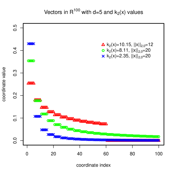
The fact that () is a sensible measure of the block sparsity for non-idealized signals is illustrated in Figure 3. In the case that has blocks with large entries and blocks with small entries, we have , whereas .
2.2 Properties
The block sparsity measure has many appealing properties which are similar to those of the non-block sparsity measure given in [16].
- (a)
Continuity: The function is continuous on for all so that it is stable with respect to small perturbations of the signal.
- (b)
Scale-invariance: It holds that for all . As a result, relies only on relative (rather than absolute) magnitudes of the entries of .
- (c)
Non-increasing in : For any , we have
which follows from the non-increasing property of the Rényi entropy with respect to .
- (d)
Range equal to : For all as given in (2) and all , we have
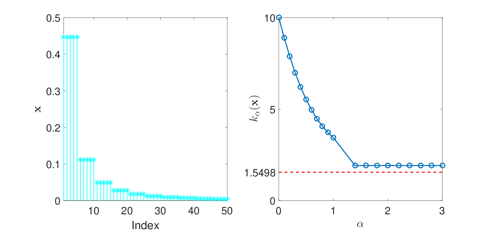
To illustrate the properties of this block sparsity measure, we show the block sparsity levels for a block compressible signal displayed in Figure 4. As we can see, for a block compressible signal with very small but non-zero entries, with a proper provided a better block sparsity measure compared to the traditional . In addition, the block sparsity level is non-increasing with respect to and its value range is between and .
2.3 An Error Bound in terms of
Before presenting the estimation procedure for the and with , we give the block sparse signal recovery results in terms of . To recover the block sparse signal in CS model (1), here we use the following mixed norm optimization algorithm proposed in [10, 12]:
| (5) |
where and is an upper bound on the noise level . Then, we have the following result concerning the robust recovery for block sparse signals.
Lemma 2
([12]) Let be noisy measurements of a vector and fix a number . Let denote the best block -sparse approximation of , such that is block -sparse and minimizes over all the block -sparse vectors , and let be a solution to (5), a Gaussian random matrix of size with entries , and block sparse signals over , where for some integer . Then, there are constants , such that with probability at least , we have
| (6) |
whenever .
Remark 1. Note that the first term on the right-hand side of (6) results from the fact that is not exactly block -sparse, while the second term quantifies the recovery error due to the measurement noise. When the block size , this lemma goes to the conventional CS result for non-block sparse signal recovery. Explicit use of block sparsity reduces the required number of measurements from to by times.
However, the relative error bound established above has the drawback that the ratio term is often unknown. As a result, it is unclear how large should be chosen to make the relative error small. In order to address this issue, in the following lemma we present an upper bound for the relative error in terms of and the new estimable block sparsity measure .
Lemma 3
Let be noisy measurements of a vector , and let be a solution to (5), a Gaussian random matrix of size with entries , and block sparse signals over , where for some integer . Then, there are constants such that with probability at least , we have
| (7) |
whenever and satisfy .
3 Block Sparsity Estimation
Let us now turn to the estimation of block sparsity with . There are two reasons to consider this interval. One is that small is usually a better block sparsity measure than very large in applications. And we can approximate by with very small as will be shown later. The other reason is that our estimation method relies on the -stable distribution, which requires to lie in . The core idea to obtain the block sparsity estimators is using random projections. In contrast to the conventional non-block sparsity estimation by using projections with univariate symmetric -stable random variables [16, 37], we use projections with multivariate centered isotropic symmetric -stable random vectors for the block sparsity estimation.
3.1 Multivariate Isotropic Stable Distribution
We start with the definition of multivariate centered isotropic symmetric -stable distribution.
Definition 2
Remark 2. The most well-known example of multivariate centered isotropic symmetric stable distribution is the case of (Multivariate Independent Gaussian Distribution), and in this case, the components of the Multivariate Gaussian random vector are independent. Another case is (Multivariate Spherical Symmetric Cauchy Distribution [27]), unlike the Multivariate Independent Gaussian case, the components of Multivariate Spherical Symmetric Cauchy random vector are uncorrelated, but dependent. The perspective and contour plots for the densities of these two cases are illustrated in Figure 5. The multivariate centered isotropic symmetric -stable random vector is a direct extension of the univariate symmetric -stable random variable, which is the special case when the dimension parameter . In practice, to simulate a -dimensional random vector from the multivariate centered isotropic symmetric -stable distribution , we can adopt the fact that , where is an independent univariate positive -stable random variable and is a standard -dimensional Gaussian random vector, see [24] for more details.

3.2 Estimation Procedure
The most important finding in our paper is that by adopting random projections using i.i.d. multivariate centered isotropic symmetric -stable random vectors, we can directly generalize the estimation procedure for the non-block sparsity measure given in [16] and obtain the estimators for and with . In the subsection that follows, we will present the corresponding estimation procedure.
We estimate the based on the random linear projection measurements:
| (9) |
where is an i.i.d. random vector, and with i.i.d. drawn from . The noise terms are i.i.d. generated from a distribution with its characteristic function being . The variable sets and are independent. In addition, we assume that are symmetric about , with , but they may have infinite variance. We impose a minor technical constraint on that the roots of its characteristic function are isolated (i.e. no limit points). It is easy to verify that many families of distributions, including Gaussian, Student’s , Laplace, uniform, and stable laws, satisfy this condition. For simplicity, throughout this paper we assume that the noise scale parameter and the distribution are known .
Because our work involves multiple values of , next we will use instead of to avoid confusion. Before proceeding to the detailed estimation procedure for and , it is necessary to obtain the following key lemma that establishes the relationship between the multivariate isotropic -stable distribution and the mixed norm .
Lemma 4
Let be fixed, and suppose with i.i.d. drawn from with and . Then, the random variable has the distribution .
Remark 3. If has different block lengths which are respectively, then we need to choose the projection random vector with i.i.d. drawn from . In that case, the conclusion in this lemma and all the results in what follows still hold without any modifications.
Remark 4. Lemma 1 in [16] is a special case of this lemma when the block size is one.
From this lemma, we can get that if with a set of i.i.d. measurement random vectors given as mentioned above, then is an i.i.d. sample from the distribution . Therefore, the problem of estimating the norm from noiseless random linear measurements reduces to a problem of estimating the scale parameter of a univariate stable distribution from an i.i.d. sample.
Now we are ready to extend this idea and present the estimation procedure for and by adopting the characteristic function method [16, 19, 20]. We use two separate sets of measurements to estimate and with their corresponding estimators denoted as and . We denote the sample sizes of these two measurements by and , respectively. In order to simplify the discussion, we only introduce the procedure to obtain for any with being a special case. We suggest the following estimator for with by integrating these two estimators and :
| (10) |
With regard to the estimation of based on the noisy random linear projection measurements (9), the characteristic function of has the form:
| (11) |
where . Then, we have the estimation equation
By adopting the empirical characteristic function
to estimate , we are able to obtain the estimator of given by
| (12) |
when and .
3.3 Asymptotic Properties
This subsection draws together the large sample properties for the proposed estimators. Let the noise-to-signal ratio constant be . We have the following uniform central limit theorem (CLT) [9] for .
Theorem 3.1
Let and be any function of such that
| (13) |
as for some finite constant and . Then, it holds that
| (14) |
as , where the limiting variance is strictly positive and defined by
| (15) |
Because it is easy to implement and produces a fairly good estimator, throughout this paper we use as our , where is any number such that for all and is the median absolute deviation statistic. Then we can obtain the consistent estimator of a constant , where random variable (see the Proposition 3 in [16]), and the consistent estimator of , . Therefore, the consistent estimator of the limiting variance is .
According to these results, we can derive the following corollary, in which a confidence interval for is constructed.
Corollary 1
Under the conditions of Theorem 1, as , we have
| (16) |
Consequently, the asymptotic confidence interval for is
| (17) |
where is the -quantile of the standard normal distribution.
It should be noted that the simple confidence interval given above is obtained using a CLT for the reciprocal via the delta method. Following this corollary, we are ready to obtain the asymptotic results for with , by combining the estimators and with their corresponding values. For each , we make the assumption that there is a constant , such that as ,
Theorem 3.2
Let and assume that the conditions of Theorem 1 hold. Then as , we have
| (18) |
where . Consequently, the asymptotic confidence interval for is
| (19) |
where is the -quantile of the standard normal distribution.
3.4 Estimating by with Small
This subsection presents the approximation of to when is close to . We begin with defining the block dynamic range (BDNR) of a non-zero signal (as given in (2)) by
| (20) |
where denotes the smallest norm of the non-zero block of . Note that our includes the dynamic range (DNR) defined in [16] as a special case of block size . Then we obtain the approximation result as follows.
Theorem 3.3
Let , is non-zero signal as given in (2), and let be any real number. Then, it holds that
| (21) |
Remark 5. Note that the approximation result established above involves no randomness and it applies to any estimator . The first term on the right-hand side of (21) can be controlled by Theorem 2, when is chosen as our proposed estimator . The second term on the right-hand side of (21) is the approximation error, which decreases as decreases. In addition, when the norms of the signal’s blocks are similar, the quantity of will not be too large so that the bound behaves well and estimating is of interest. Whereas, if there is a big difference in the norms of the signal’s blocks, then will be very large such that may not be the best block sparsity measure to estimate.
4 Simulations
In this section, we conduct numerical experiments to illustrate our theoretical results. We start with the discussion of , that is, we use to estimate the block sparsity measure . To obtain the estimator , we require a set of measurements by using the multivariate centered isotropic symmetric Cauchy projection, and a set of measurements by using the multivariate centered isotropic symmetric Gaussian projection. The samples and are generated as:
| (22) |
where with being i.i.d. random vector, and with i.i.d. drawn from with . Similarly, with being i.i.d. random vector, and with i.i.d. drawn from with . The noise terms and are generated with i.i.d entries from a standard normal distribution. In this set of experiments, we consider a sequence of pairs for the sample sizes . For each experiment, we replicated times. Consequently, we have realizations of for each . Throughout all the experiments, we fix .
4.1 Exactly Block Sparse Case
First, we let our signal be the following simple exactly block sparse vector
where is a vector of length with entries all ones, is the zero vector of length . Then it is obvious that , while and depend on the block size that we choose. Under this exactly block sparse setting, we have performed the following two simulation studies on the error dependence on the parameters and the asymptotic normality of the proposed estimators.
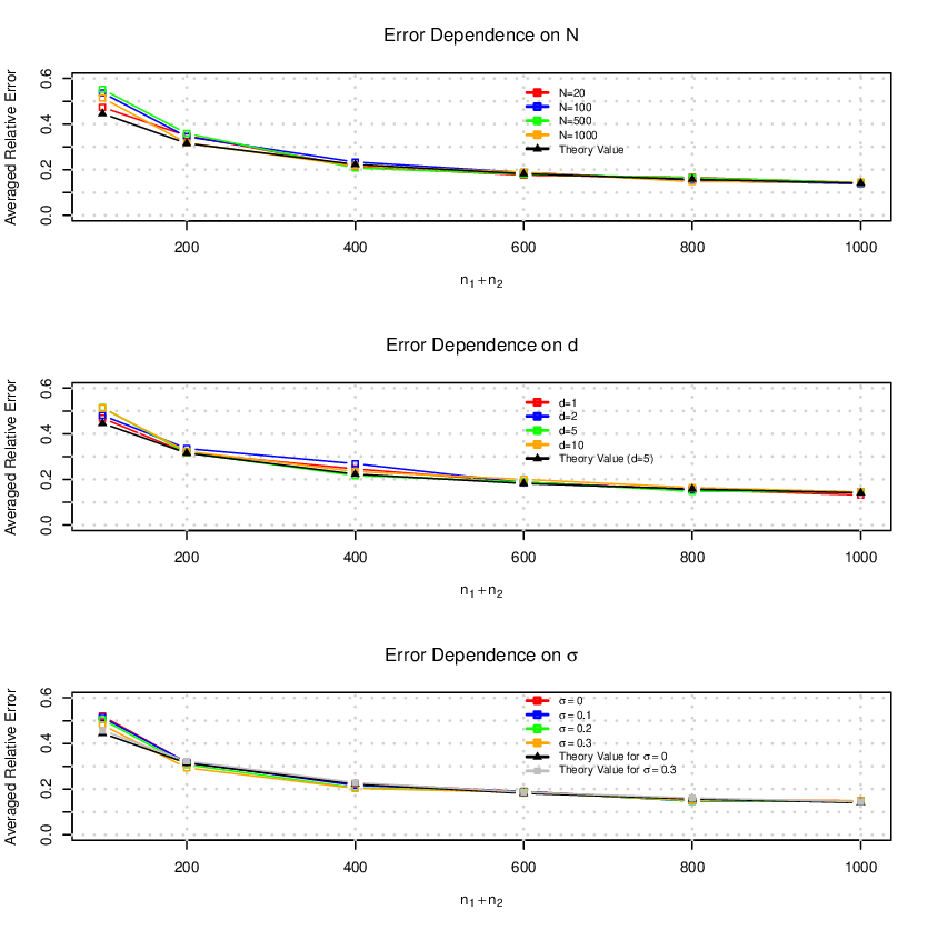
a) The first simulation study in this part is conducted to illustrate the influence of varying the parameter settings. It is done with a variety of parameters, like , and , each of which corresponds to a separate plot in Figure 6. Except in the top plot where , the signal dimension is set to . The block size is set to in all cases, except in the middle plot where , which corresponds to the true value (here also equals , the exact block sparsity level of our signal with the block size set to ). In all cases, , except in the bottom plot where .
The quantities are averaged over the replications as an approximation of . According to Theorem 2, we get , where is a standard normal random variable and . Then the fact that implies that the theoretical curves for are simply , as a function of . It should be note that depends on and , but not on .
From Figure 6, we can see that the theoretical curves (black) coincide well with the empirical ones (colored). Moreover, the averaged relative error does not depend on or (when is fixed), as expected from Theorem 2, and its dependence on the is also negligible.
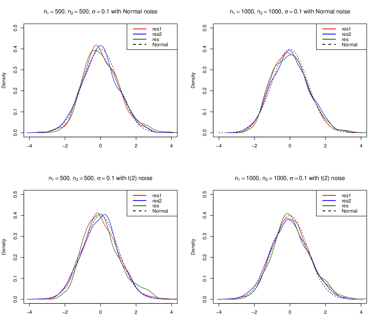
b) Meanwhile, the second simulation study in this part has been conducted to illustrate the asymptotic normality of our estimators in Corollary 1 and Theorem 2. We have replications for these experiments, that is, we have samples of the standardized statistics , and . We consider four cases, with and the noise distribution is standard normal and which has infinite variance. In all these cases, we fix , , and .
Figure 7 shows that all the probability density curves of the standardized statistics are very close to the standard normal density curve, which verifies our theoretical results. And these results hold even when the noise distribution is heavy-tailed. Comparing these four plots, it can be observed that the normal approximation improves as the sample size increases or the noise variance decreases.
4.2 Nearly Block Sparse Case
Second, we consider our signal to be not exactly block sparse but nearly block sparse, i.e., the entries of -th block all equal , with chosen so that . In this case, the norms of the signal’s blocks decay like for . Figure 8 and Figure 9 display simulation results that are similar to those obtained in the exactly block sparse case, using the same settings as in the previous subsection.


4.3 Estimating by with Small
Third, we consider the estimation of the mixed norm by using with . We consider the signal of the form
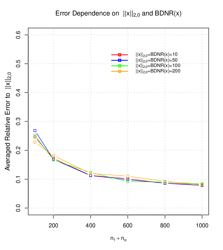
with chosen so that . In this set of experiments, we fix and . To obtain , we generate the samples and , where with being i.i.d. random vector, and with i.i.d. drawn from with . Similarly, with being i.i.d. random vector, and with i.i.d. drawn from with . The noise terms and are generated with i.i.d. entries from a standard normal distribution. The noise level is set to . We consider a sequence of pairs for the sample sizes . For each experiment, we replicate times. Then, we have realizations of for each . We vary and , and average the quantities . Specifically, we consider the four cases with .
As expected in Theorem 3, it can be seen from Figure 10 that accurately estimates across a broad set of parameters and , and these parameters have a very limited effect on the relative estimation error.
5 Conclusion
In this paper, we consider the estimation of block sparsity in compressive sensing, which is crucial from both theoretical and practical points of view. We introduced a new soft measure of block sparsity and developed its estimators by using multivariate centered isotropic symmetric -stable random projections. The asymptotic properties of the estimators were established. A series of numerical experiments illustrated our theoretical results.
There are some interesting issues left for future research. Throughout the paper, we assume that the noise scale parameter and the characteristic function of noise are known. In practice, however, they are usually unknown and need to be estimated. Although [16] considered the effects of adopting their estimators in the estimation procedure, how to estimate these parameters based on our random linear projection measurements itself is still unknown. In addition, we have been considering the sparsity and block sparsity estimations for real-valued signals so far. It will be interesting to generalize the existing results to the case of complex-valued signals.
Appendix Proofs
Our main theoretical findings Theorem 1 and Theorem 2 follow from Theorem 2 and Corollary 1 in [16], because in these two estimation procedures, the noiseless measurements after random projections both have univariate symmetric stable distributions, but with different scale parameters, i.e., for the non-block sparsity estimation in [16] and for the block sparsity estimation in the present paper. Therefore, the asymptotic results for the scale parameters estimation by using the characteristic function method are rather similar. In order not to repeat, all the details are omitted. Here we only present the proofs of Lemma 3, Lemma 4 and Theorem 3.
Proof of Lemma 3. The proof procedure follows from the proof of Proposition 1 in [16] with some careful modifications. We will use the same as in Lemma 2 and some number that satisfies
| (23) |
In Lemma 2, we choose with . It is worth noting that when , this is at most , and thus lies in . Then we have
by using our assumption that . Therefore, it is easy to verify that our choice of fulfills .
Next, we let be as in Lemma 2 so that (6) holds with probability at least . Moreover, it holds that
Thus, with and being the same as in (6), we get
Finally, the proof is completed by setting , and noticing the fact that .
Proof of Lemma 4. By using the independence of , for , the characteristic function of has the form:
Then, this lemma follows from Definition 2.
Proof of Theorem 3. The proof technique of this theorem is adopted from the proof of Proposition 5 in [16]. We reproduce the proof procedure for the sake of completeness. Combining the triangle inequality that
and the fact that , we get
Thus, to prove Theorem 3, it suffices to bound the last term on the right-hand side. Next, according to the fact that and that is a non-increasing function of , it follows that
Our task now is to derive a bound on . For any , and , let us introduce the probability vector with and defined as in Section 2.1. Then, according to the definition of , we infer that
provided that and the formula for given in the book [2] (page 72). Furthermore, since and , then for any with , we have
where . As a result, for all and , it holds that
due to . Hence, the proof is completed according to the basic integral result .
References
- (1) Baraniuk, R.G., Cevher, V., Duarte, M.F., Hegde, C.: Model-based compressive sensing. IEEE Transactions on Information Theory 56(4), 1982–2001 (2010)
- (2) Beck, C., Schögl, F.: Thermodynamics of chaotic systems: an introduction. 4. Cambridge University Press (1995)
- (3) Blumensath, T., Davies, M.E.: Iterative hard thresholding for compressed sensing. Applied and Computational Harmonic Analysis 27(3), 265–274 (2009)
- (4) Blumensath, T., Davies, M.E.: Sampling theorems for signals from the union of finite-dimensional linear subspaces. IEEE Transactions on Information Theory pp. 1872–1882 (2009)
- (5) Chen, J., Huo, X.: Theoretical results on sparse representations of multiple-measurement vectors. IEEE Transactions on Signal processing 54(12), 4634–4643 (2006)
- (6) Chen, S.S., Donoho, D.L., Saunders, M.A.: Atomic decomposition by basis pursuit. SIAM Journal on Scientific Computing 20, 33–61 (1998)
- (7) Cotter, S.F., Rao, B.D., Engan, K., Kreutz-Delgado, K.: Sparse solutions to linear inverse problems with multiple measurement vectors. IEEE Transactions on Signal Processing 53(7), 2477–2488 (2005)
- (8) Duarte, M.F., Eldar, Y.C.: Structured compressed sensing: From theory to applications. IEEE Transactions on Signal Processing 59(9), 4053–4085 (2011)
- (9) Dudley, R.M.: Uniform central limit theorems, vol. 63 of cambridge studies in advanced mathematics (1999)
- (10) Eldar, Y.C., Kuppinger, P., Bolcskei, H.: Block-sparse signals: Uncertainty relations and efficient recovery. IEEE Transactions on Signal Processing 58(6), 3042–3054 (2010)
- (11) Eldar, Y.C., Kutyniok, G.: Compressed Sensing: Theory and Applications. Cambridge University Press (2012)
- (12) Eldar, Y.C., Mishali, M.: Robust recovery of signals from a structured union of subspaces. IEEE Transactions on Information Theory 55(11), 5302–5316 (2009)
- (13) Elhamifar, E., Vidal, R.: Block-sparse recovery via convex optimization. IEEE Transactions on Signal Processing 60(8), 4094–4107 (2012)
- (14) Foucart, S., Rauhut, H.: A Mathematical Introduction to Compressive Sensing, vol. 1. Birkhäuser Basel (2013)
- (15) Lopes, M.: Estimating unknown sparsity in compressed sensing. In: International Conference on Machine Learning, pp. 217–225 (2013)
- (16) Lopes, M.E.: Unknown sparsity in compressed sensing: Denoising and inference. IEEE Transactions on Information Theory 62(9), 5145–5166 (2016)
- (17) Lv, X., Bi, G., Wan, C.: The group lasso for stable recovery of block-sparse signal representations. IEEE Transactions on Signal Processing 59(4), 1371–1382 (2011)
- (18) Majumdar, A., Ward, R.K.: Compressed sensing of color images. Signal Processing 90(12), 3122–3127 (2010)
- (19) Markatou, M., Horowitz, J.L.: Robust scale estimation in the error-components model using the empirical characteristic function. Canadian Journal of Statistics 23(4), 369–381 (1995)
- (20) Markatou, M., Horowitz, J.L., Lenth, R.V.: Robust scale estimation based on the the empirical characteristic function. Statistics & probability letters 25(2), 185–192 (1995)
- (21) Mishali, M., Eldar, Y.C.: Reduce and boost: Recovering arbitrary sets of jointly sparse vectors. IEEE Transactions on Signal Processing 56(10), 4692–4702 (2008)
- (22) Mishali, M., Eldar, Y.C.: Blind multiband signal reconstruction: Compressed sensing for analog signals. IEEE Transactions on Signal Processing 57(3), 993–1009 (2009)
- (23) Needell, D., Tropp, J.A.: CoSaMP: Iterative signal recovery from incomplete and inaccurate samples. Applied and Computational Harmonic Analysis 26(3), 301–321 (2009)
- (24) Nolan, J.P.: Multivariate elliptically contoured stable distributions: theory and estimation. Computational Statistics 28(5), 2067–2089 (2013)
- (25) Parvaresh, F., Vikalo, H., Misra, S., Hassibi, B.: Recovering sparse signals using sparse measurement matrices in compressed dna microarrays. IEEE Journal of Selected Topics in Signal Processing 2(3), 275–285 (2008)
- (26) Plan, Y., Vershynin, R.: One-bit compressed sensing by linear programming. Communications on Pure and Applied Mathematics 66(8), 1275–1297 (2013)
- (27) Press, S.J.: Multivariate stable distributions. Journal of Multivariate Analysis 2(4), 444–462 (1972)
- (28) Stojnic, M., Parvaresh, F., Hassibi, B.: On the reconstruction of block-sparse signals with an optimal number of measurements. IEEE Transactions on Signal Processing 57(8), 3075–3085 (2009)
- (29) Tropp, J.A., Gilbert, A.C.: Signal recovery from random measurements via orthogonal matching pursuit. IEEE Transactions on Information Theory 53(12), 4655–4666 (2007)
- (30) Vershynin, R.: Estimation in high dimensions: a geometric perspective. In: Sampling theory, a renaissance, pp. 3–66. Springer (2015)
- (31) Yuan, M., Lin, Y.: Model selection and estimation in regression with grouped variables. Journal of the Royal Statistical Society: Series B (Statistical Methodology) 68(1), 49–67 (2006)
- (32) Zeinalkhani, Z., Banihashemi, A.H.: Iterative reweighted recovery algorithms for compressed sensing of block sparse signals. IEEE Transactions on Signal Processing 63(17), 4516–4531 (2015)
- (33) Zhou, Z.: Block sparse signal recovery via minimizing the block -ratio sparsity. arXiv preprint arXiv:2103.07145 (2021)
- (34) Zhou, Z., Yu, J.: On -ratio CMSV for sparse recovery. Signal Processing 165, 128–132 (2019)
- (35) Zhou, Z., Yu, J.: Recovery analysis for weighted mixed minimization with . Journal of Computational and Applied Mathematics 352, 210–222 (2019)
- (36) Zhou, Z., Yu, J.: Sparse recovery based on -ratio constrained minimal singular values. Signal Processing 155, 247–258 (2019)
- (37) Zolotarev, V.M.: One-dimensional stable distributions, vol. 65. American Mathematical Soc. (1986)