A Conforming Primal-Dual Mixed Formulation
for the 2D Multiscale Porous Media Flow Problem

A Conforming Primal-Dual Mixed Formulation for the 2D Multiscale Porous Media Flow Problem

A Conforming Primal-Dual Mixed Formulation
for the 2D Multiscale Porous Media Flow Problem

1 Introduction

2 Preliminaries

3 The Discretization of the Problem

4 Numerical Examples

5 Conclusions and Final Discussion

Acknowledgements

References

1 Introduction

2 Preliminaries

3 The Discretization of the Problem

4 Numerical Examples

5 Conclusions and Final Discussion

Acknowledgements

References

2.1 Geometric Setting

2.2 The Strong Problem and its Continuous Weak Formulation

3.1 Strong Convergence

3.2 Rate of Convergence

2.1 Geometric Setting

2.2 The Strong Problem and its Continuous Weak Formulation

3.1 Strong Convergence

3.2 Rate of Convergence

Abstract

Keywords:

2010 MSC

Definition 1

Hypothesis 1

Definition 2

Definition 3

Theorem 1

Lemma 2

Proof 1

Remark 1

Hypothesis 2

Theorem 3

Proof 2

Theorem 4

Proof 3

Theorem 5

Proof 4

Lemma 6

Proof 5

Lemma 7

Proof 6

Theorem 8

Proof 7

Proposition 9

Proof 8

Proposition 10

Proof 9

Theorem 11

Proof 10

Corollary 12

Proposition 13

Proof 11

Theorem 14

Proof 12

Theorem 15

Proof 13

Definition 4

Remark 2

Theorem 16

Proof 14

Theorem 17

Proof 15

Remark 3

Example 1

Example 2

Example 3

Example 4

Abstract

Keywords:

2010 MSC

Definition 1

Hypothesis 1

Definition 2

Definition 3

Theorem 1

Lemma 2

Proof 1

Remark 1

Hypothesis 2

Theorem 3

Proof 2

Theorem 4

Proof 3

Theorem 5

Proof 4

Lemma 6

Proof 5

Lemma 7

Proof 6

Theorem 8

Proof 7

Proposition 9

Proof 8

Proposition 10

Proof 9

Theorem 11

Proof 10

Corollary 12

Proposition 13

Proof 11

Theorem 14

Proof 12

Theorem 15

Proof 13

Definition 4

Remark 2

Theorem 16

Proof 14

Theorem 17

Proof 15

Remark 3

Example 1

Example 2

Example 3

Example 4

Journal: arXiv

Fernando A Morales Email: famoralesj@unal.edu.co Address: Escuela de Matemáticas Universidad Nacional de Colombia, Sede Medellín
Calle 59 A No 63-20 - Bloque 43, of 106, Medellín - Colombia

In this paper a new primal-dual mixed finite element method is introduced, aimed to model multiscale problems with several geometric subregions in the domain of interest. In each of these regions porous media fluid flow takes place, but governed by physical parameters at a different scale; additionally, a fluid exchange through contact interfaces occurs between neighboring regions. The well-posedness of the primal-dual mixed finite element formulation on bounded simply connected polygonal domains of the plane is presented. Next, the convergence of the discrete solution to the exact solution of the problem is discussed, together with the convergence rate analysis. Finally, the numerical examples illustrate the method’s capabilities to handle multiscale problems and interface discontinuities as well as experimental rates of convergence.

coupled discontinuous Darcy system, mixed formulations, multi scale problems.

65M60 , 35J50 , 65N12

Mixed variational formulations are a very important topic of research in applied mathematics. The Babuska-Brezzi theory (see Theorem 1) is remarkably powerful from the theoretical point of view, however it introduces high complexity in the discrete finite element spaces approximating the solution; this reflects in numerical stability problems (see [1]). The achievements to overcome such difficulty can be on several directions. One of the streams seeks to stabilize the approximation by modifying the bilinear forms involved, namely using symmetric properties of the tensors as in [2], [3], or including terms in the bilinear forms in a “balanced" way as in[4], [1]. As this technique has proved to be fruitful and rich in terms of the possibilities to stabilize the forms of interest, some other aspects arise by itself, such as the discussion of minimal stabilisation procedures (see [5]), or the a-priori, a-posteriori error analysis for these new scheme (see [2]). A second approach uses discontinuous Galerkin finite elements (DG). The DG methods have several advantages and goals, some of these are: addressing non-conformality in a more flexible way, treating stability issues due to coupling constraints (demanding regularity in the discrete spaces), and computing in a more accurate way the physical quantity that is known to be predominant in specific subregions. The latter is attained in two ways, by local refining of the mesh and by approximating polynomial spaces; see [6], [7] for a unified vision of the DG Methods.

All the aforementioned works, whichever the problem they may be analyzing (elasticity, heat diffusion, free flow, Darcy flow, etc), treat separately the primal and dual mixed formulations (see [8], [9], [10]). The present paper is focused on using simultaneously both fundamental versions for the treatment of multiscale problems in Darcy flow (see Problem (1)), it is therefore a primal-dual mixed formulation; in a way this article is the numerical implementation of the formulation introduced in [11] (see also [12], [13] for related formulations). The stability aspects become particularly critical when dealing with multiscale problems, as the presence of physical coefficients with different orders of magnitude adds up to the built-in complexity of the mixed variational formulations (coefficient $a(\cdot)$ in Problem (1)). The primal-dual mixed formulation tackles this issue by removing coupling constraints from the discrete trial spaces while satisfying them only on the solution i.e., the continuous formulation replaces strong coupling conditions by weak coupling conditions (see Equations (7) and Problem (14)). Replacing the nature of the coupling conditions is a strategy already used in DG methods using penalization techniques; however, this is done only on the discrete version, while the continuous formulation still relies on strong coupling conditions. The latter is because, in the Darcy flow problem, while the primal mixed formulation can introduce weak coupling conditions on the normal flow exchange, the normal stress has to stay continuos. In contrast, the dual mixed formulation can introduce weak coupling conditions for the normal stress balance, but it requires the normal flow exchange to be continuous. The continuity constraints of the classical mixed formulations reflect later on, in the deep discussions of convergence present in the DG methods.

Another advantage of the discrete primal-dual mixed formulation we are to introduce in this work is that, according to the regions, the predominant effect can be chosen to be modeled with the discrete space holding the sense of continuity, while the secondary effect is modeled with the discontinuous space. In the case of Darcy flow, the pressure is the dominant effect in regions of low permeability, while the flow velocity is the predominant one in regions of high permeability (see Figures 4, 6 and 10). This concept has already araised naturally in previous DG methods coupling advection with diffusion phenomena, due to the discrete spaces involved in the formulations, see [14]. To the author’s best knowledge there is no precedent for having this level of flexibility in the analysis of coupling fluid flow phenomena, as the literature analyzing multiscale flow is mainly focused in coupling Stokes flow with Darcy flow, see [15], [16], [17], [18], [19].

The proposed model is to analyze a variation of the classic porous media problem on a connected bounded open region $\Omega\subset\bm{\mathbbm{R}}^{2}$ , i.e.,

	$a(\cdot)\,\mathbf{u}+\bm{\nabla}p+\mathbf{g}=0\,,$		(1a)
	$\bm{\nabla}\cdot\mathbf{u}=F\,\quad\mathrm{in}\;\Omega.$		(1b)
	$p=0\,\quad\mathrm{on}\;\Gamma_{d},$		(1c)
	$\mathbf{u}\cdot\bm{\widehat{n}}=0\quad\mathrm{on}\;\Gamma_{f}\overset{\mathbf{def}}{=}\partial\Omega-\Gamma_{d};$		(1d)

more specifically, when $\Omega$ is partitioned in two subdomains $\Omega_{1},\Omega_{2}$ such that $a(\cdot)\big|_{\Omega_{1}}=O(1)$ and $a(\cdot)\big|_{\Omega_{2}}=O(\epsilon)$ for $\epsilon>0$ small (see Figure 1). Recall that $a(\cdot)$ is the flow resistance i.e., the viscosity times the inverse of permeability of the porous medium. Systems such as this, are suited for the modeling of oil reservoirs and subsurface water, where a network of thin channels, embedded in bedrock occurs, therefore the flow resistance coefficient changes its order of magnitude from one region $\Omega_{1}$ to the other $\Omega_{2}$ . In this context the continuity of the solution $[\mathbf{u},p]$ across the interface between $\Omega_{1}$ and $\Omega_{2}$ becomes a liability from the numerical point of view. Therefore, if it is possible to estimate a-priori, the magnitude of change that the solution will experience from one subdomain to the other (see Example 4), it is a more strategic approach to artificially introduce a discontinuity across the interface, and model it with a system, see Equations (6), satisfying a balance/coupling condition for both, normal flux and normal stress, see Equations (7). As mentioned above, these exchange conditions will be introduced weakly in the formulation allowing full decoupling of the underlying function spaces. Moreover, the trial spaces require that the pressure $q$ is only square integrable $L^{2}$ on one side of the interface, while it belongs to $H^{1}$ on the other side of the interface (see Figure 4 (a)); such discontinuity on the test spaces is ideal to handle discontinuities on the normal stress across the interface. The analogous takes place on the velocities modeling spaces, here the test functions $\mathbf{v}$ belong to $\mathbf{H_{div}}$ on one side of the interface while they are only square integrable $\mathbf{L}^{2}$ on the other (see Figure 4 (b)). Again, this scenario will be ideal for discontinuities of normal flux across the interface. In summary, the primal-dual mixed formulation method will be able to capture interface discontinuities using uncoupled, conforming, finite dimensional spaces, presented in Definitions 17 and 18.

We close this section introducing the general notation. In the present work vectors are denoted by boldface letters as are vector-valued functions and corresponding function spaces. The symbols $\bm{\nabla}$ and $\bm{\nabla}\cdot$ represent the gradient and divergence operators respectively. The dimension is indicated by $N$ which will be equal to $2$ or $3$ depending on the context. Given a function $f:\bm{\mathbbm{R}}^{N}\rightarrow\bm{\mathbbm{R}}$ then $\int_{\mathcal{M}}f\,dS$ denotes the integral on the $N-1$ dimensional manifold $\mathcal{M}\subseteq\bm{\mathbbm{R}}^{\!N}$ . Analogously, $\int_{A}f\,d\mathbf{x}$ stands for the integral in the set $A\subseteq\bm{\mathbbm{R}}^{\!N}$ ; whenever the context is clear we simply write $\int_{A}f$ . Given an open set $G$ of $\bm{\mathbbm{R}}^{N}$ , the symbols $\|\cdot\|_{0,G}$ , $\|\cdot\|_{1,G}$ , $\|\cdot\|_{1/2,\partial G}$ , $\|\cdot\|_{-1/2,\partial G}$ and $\|\cdot\|_{\mathbf{H_{div}}(G)}$ denote the $L^{2}(G)$ , $H^{1}(G)$ , $H^{1/2}(\partial G)$ , $H^{-1/2}(\partial G)$ and $\mathbf{H_{div}}(G)$ norms respectively, while $|M|$ represents the Lebesgue measure of $G$ in $\bm{\mathbbm{R}}$ , $\bm{\mathbbm{R}}^{2}$ or $\bm{\mathbbm{R}}^{3}$ depending on the context.

In this section we set the conditions on the domain of reference as well as its gridding.

Given a bounded open set $\omega$ in $\bm{\mathbbm{R}}^{2}$ we will say that a bipartite map is a finite collection of connected open subsets $\mathcal{G}=\{G_{n}:1\leq n\leq N\}$ such that

(i)

If $n\neq k$ then $G_{n}\cap G_{k}=\emptyset$ .
(ii)

The union satisfies $\Big|\omega-\bigcup\limits_{i\,=\,1}^{N}G_{n}\Big|=0$ and $\cl(\omega)=\bigcup\limits_{i\,=\,1}^{N}\cl(G_{n})$ .
(iii)
The collection $\mathcal{G}=\big\{G_{n}:1\leq n\leq N\big\}$ is partitioned in two subcollections $\mathcal{G}_{1}=\big\{G^{\,1}_{i}:1\leq i\leq I\big\}$ and $\mathcal{G}_{2}=\big\{G^{\,2}_{j}:1\leq j\leq J\big\}$ such that
1. a)
  
  $\big\{G_{n}:1\leq n\leq N\big\}=\big\{G^{1}_{i}:1\leq i\leq I\big\}\cup\big\{G^{2}_{j}:1\leq j\leq J\big\}$ .
2. b)
  
  If $i\neq k$ then $\big|\partial G^{1}_{i}\cap\partial G^{1}_{k}\big|=0$ .
3. c)
  
  If $j\neq\ell$ then $\big|\partial G^{\,2}_{j}\cap\partial G^{\,2}_{\ell}\ \big|=0$ .
The collections $\mathcal{G}_{1}$ and $\mathcal{G}_{2}$ are said to be the bipartition or the bi-coloring of the map.

The domain of interest $\Omega$ is a polygonal, bounded, connected region of the plane and, it satisfies that

(i)

It has a bipartite map $\mathcal{G}=\{G_{n}:1\leq n\leq N\}$ such that $G_{n}$ is a polygon for each $n=1,\ldots,N$ .
(ii)

If $\mathcal{G}_{1},\mathcal{G}_{2}$ is the bipartition of the map $\mathcal{G}$ then $\cl\big[\bigcup\{L:L\in\mathcal{G}_{1}\}\big]$ and $\cl\big[\bigcup\{L:L\in\mathcal{G}_{2}\}\big]$ are connected.

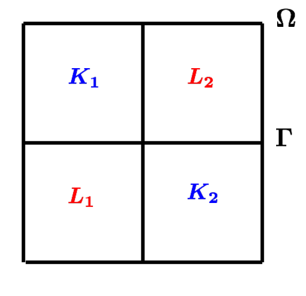
An example of bipartite map is depicted in Figure 1 (a), together with some other concepts introduced in the following definition.

Let $\Omega$ satisfy Hypothesis 1 and let $\mathcal{G}=\{G_{n}:1\leq n\leq N\}$ be its bipartite map with $\mathcal{G}_{1}$ , $\mathcal{G}_{2}$ the map bipartition.

(i)

For each polygon $K\in\mathcal{G}$ denote by $\bm{\widehat{\nu}}$ the outer normal vector to its boundary $\partial K$ .

(ii)

For each polygon $K\in\mathcal{G}$ define $\bm{\widehat{n}}$ by

\bm{\widehat{n}}(\mathbf{x})\overset{\mathbf{def}}{=}\begin{cases}\bm{\widehat{\nu}}(\mathbf{x})&K\in\mathcal{G}_{1}\;\text{and}\;\mathbf{x}\in\partial K,\\ -\bm{\widehat{\nu}}(\mathbf{x})&K\in\mathcal{G}_{2}\;\text{and}\;\mathbf{x}\in\partial K\cap\Omega,\\ \bm{\widehat{\nu}}(\mathbf{x})&K\in\mathcal{G}_{2}\,\text{and}\;\mathbf{x}\in\partial K\cap\partial\Omega.\end{cases}

(2)

(iii)

Define $\displaystyle\Omega_{1}\overset{\mathbf{def}}{=}\bigcup\{L:L\in\mathcal{G}_{1}\}$ and $\displaystyle\Omega_{2}\overset{\mathbf{def}}{=}\bigcup\{M:M\in\mathcal{G}_{2}\}$ .
(iv)

Denote by $\displaystyle\Gamma\overset{\mathbf{def}}{=}\bigcup\{\partial K:K\in\mathcal{G}\}-\partial\Omega$ , the interface of the domain.

Refer to caption — (a) Bipartite Map $\mathcal{G}$ of region $\Omega$ .

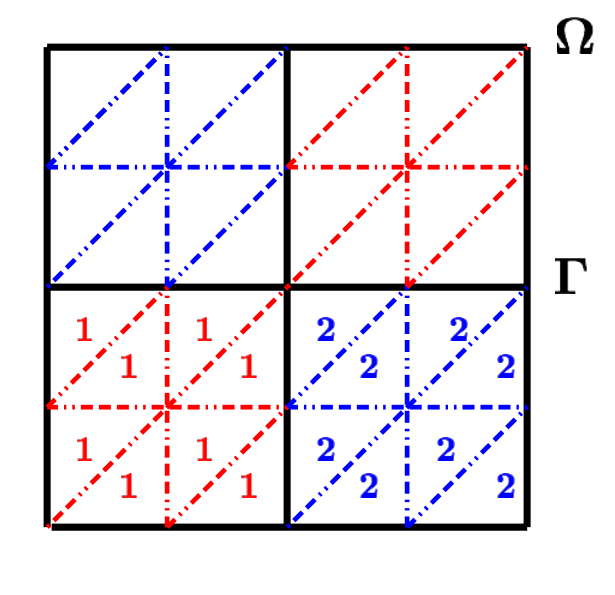
Next, we define the type of grids that will be considered in this work, see Figure 1 (b) for a simple example.

Let $\Omega$ be as in Definition 2 above, then

(i)

A triangulation $\mathcal{T}$ of the domain $\Omega$ is said to be consistent with the map $\mathcal{G}=(\mathcal{G}_{1},\mathcal{G}_{2})$ if for each triangle $K\in\mathcal{T}$ , it holds that $K\cap\Omega_{1}=\emptyset$ or $K\cap\Omega_{2}=\emptyset$ . Equivalently, $\bm{\mathbbm{1}}_{K\cap\Omega_{1}}(\cdot)\bm{\mathbbm{1}}_{K\cap\Omega_{2}}(\cdot)=0$ .
(ii)

Given two triangulations $\mathcal{T}^{\prime}$ and $\mathcal{T}$ of the domain $\Omega$ , we say that $\mathcal{T}^{\prime}$ is a refinement of $\mathcal{T}$ , denoted by $\mathcal{T}^{\prime}\leq\mathcal{T}$ , if for each element $K^{\prime}\in\mathcal{T}^{\prime}$ there exists a triangle $K\in\mathcal{T}$ such that $K^{\prime}\subseteq K$ .
(iii)

A sequence $\{\mathcal{T}^{h}:h>0\}$ is said to be monotone if $h^{\prime}<h$ implies that $\mathcal{T}^{h^{\prime}}\leq\mathcal{T}^{h}$ .

We begin this section recalling the general abstract setting to be used in this article. Let $\mathbf{X}$ and $\mathbf{Y}$ be Hilbert spaces and let ${\mathcal{A}}:\mathbf{X}\rightarrow\mathbf{X}$ ^′, ${\mathcal{B}}:\mathbf{X}\rightarrow\mathbf{Y}$ ^′ and ${\mathcal{C}}:\mathbf{Y}\rightarrow\mathbf{Y}$ ^′ be continuous linear operators, we are to work on the following problem

\begin{split}\text{Find a pair}\;(\mathbf{x},\mathbf{y})\in\mathbf{X}\times\mathbf{Y}:\quad{\mathcal{A}}\mathbf{x}+{\mathcal{B}}^{\prime}\mathbf{y}=F_{1}\quad\text{in}\;\mathbf{X}^{\prime},\\ -{\mathcal{B}}\mathbf{x}+{\mathcal{C}}\mathbf{y}=F_{2}\quad\text{in}\;\mathbf{Y}^{\prime},\end{split}

(3)

where $F_{1}\in\mathbf{X}^{\prime}$ and $F_{2}\in\mathbf{Y}^{\prime}$ . The following is a well-known result [20].

Assume that the linear operators ${\mathcal{A}}:\mathbf{X}\rightarrow\mathbf{X}^{\prime}$ , ${\mathcal{B}}:\mathbf{X}\rightarrow\mathbf{Y}^{\prime}$ , ${\mathcal{C}}:\mathbf{Y}\rightarrow\mathbf{Y}^{\prime}$ are continuous and

(i)

${\mathcal{A}}$ is non-negative and $\mathbf{X}$ -coercive on $\ker({\mathcal{B}})$ .

(ii)

${\mathcal{B}}$ satisfies the inf-sup condition

\inf_{\mathbf{y}\,\in\,\mathbf{Y}}\sup_{\mathbf{x}\,\in\,\mathbf{X}}\frac{|{\mathcal{B}}\mathbf{x}(\mathbf{y})|}{\|\mathbf{x}\|_{\mathbf{X}}\,\|\mathbf{y}\|_{\mathbf{Y}}}>0\,.

(4)

(iii)

$C$ is non-negative symmetric.

Then for every $F_{1}\in\mathbf{X}^{\prime}$ and $F_{2}\in\mathbf{Y}^{\prime}$ the Problem (3) has a unique solution in $(\mathbf{x},\mathbf{y})\in\mathbf{X}\times\mathbf{Y}$ ; additionally it satisfies the estimate

\|\mathbf{x}\|_{\mathbf{X}}+\|\mathbf{y}\|_{\mathbf{Y}}\leq c\,(\|F_{1}\|_{\mathbf{X}^{\prime}}+\|F_{2}\|_{\mathbf{Y}^{\prime}}).

(5)

Next, we present the strong problem to be approximated. Given a region $\Omega$ verifying Hypothesis 1, we introduce the following generalization of the Darcy flow Problem (1).

	$a(\cdot)\,\mathbf{u}_{1}+\bm{\nabla}p_{1}+\mathbf{g}=0\,,$		(6a)
	$\bm{\nabla}\cdot\mathbf{u}_{1}=F\,\quad\mathrm{in}\;\Omega_{1}.$		(6b)
	$p_{1}=0\quad\mathrm{on}\;\partial\Omega_{1}\cap\partial\Omega.$		(6c)

	$a(\cdot)\,\mathbf{u}_{2}+\bm{\nabla}p_{2}+\mathbf{g}=0\,,$		(6d)
	$\bm{\nabla}\cdot\mathbf{u}_{2}=F\,\quad\mathrm{in}\;\Omega_{2}.$		(6e)
	$\mathbf{u}_{2}\cdot\bm{\widehat{n}}=0\quad\mathrm{on}\;\partial\Omega_{2}\cap\partial\Omega.$		(6f)

Endowed with the following interface exchange balance conditions

	$p_{2}-p_{1}=f_{\Sigma}\,,$		(7a)
	$\mathbf{u}_{1}\cdot\bm{\widehat{n}}-\mathbf{u}_{2}\cdot\bm{\widehat{n}}=\beta(\cdot)\,p_{2}+f_{\bm{\hat{n}}}.$		(7b)

The problem above, allows discontinuity jumps of discontinuity across the interface $\Gamma$ , due to the forcing terms in the normal stress (7a) and normal flux balance conditions (7b), both relationships are nothing but statements normal stress and normal flux balance. The coefficients $a(\cdot)$ , $\beta(\cdot)$ are nonnegative and they stand for the medium resistance to the fluid flow and the interface storage rate, respectively. The multiscaling of the coefficient $a(\cdot)$ will occur when modeling problems such as geological fissured systems (see [13]) where regions of high permeability have to be coupled with regions of low permeability. On the other hand, the coefficient $\beta(\cdot)$ is meaningful in this context when one of the regions stores fluid and the other does not, due to the difference in the scaling of the problem between regions, its determination/measurement is an active research field, see [21] for an example of related work. Finally, recall that Darcy’s law relates only pressure-velocity and that the pressure only acts in normal direction with respect to the physical object in contact, therefore the interface fluid exchange conditions (7) can only be stated in the normal direction, while it is not possible to reconcile interface tangential velocity conditions with a Darcy system, see [19] for an example.

In order to introduce the modeling spaces to be used in the weak variational formulation, first notice that $\big\{L:L\in\mathcal{T}_{1}\big\}$ , $\big\{M:M\in\mathcal{T}_{2}\big\}$ are the simply connected components of $\Omega_{1}$ and $\Omega_{2}$ respectively. Then,

\displaystyle\mathbf{H_{div}}(\Omega_{1})=\bigoplus_{L\,\in\,\mathcal{T}_{1}}\mathbf{H_{div}}(L),

\displaystyle H^{1}(\Omega_{2})=\bigoplus_{M\,\in\,\mathcal{T}_{2}}H^{1}(M).

The following space is introduced in order to couple adequately, the action of the pressure traces in the variational formulation

\begin{split}E(\Omega_{2})\overset{\mathbf{def}}{=}&\big\{q\in H^{1}(\Omega_{2}):q\bm{\mathbbm{1}}_{\partial M\cap\partial L}\in H^{1/2}(\partial L)\;\text{for all }\,(L,M)\in\mathcal{G}_{1}\times\mathcal{G}_{2}\big\}\\ =&\big\{q\in H^{1}(\Omega_{2}):q\bm{\mathbbm{1}}_{\Gamma}\in H^{1/2}(\Gamma)\big\}.\end{split}

(8)

We endow $E(\Omega_{2})$ with the $H^{1}(\Omega_{2})$ inner product. It is direct to see that $E(\Omega_{2})$ is a closed subspace of $H^{1}(\Omega_{2})$ and consequently a Hilbert space. Also define

\mathbf{V}(\Omega_{2})\overset{\mathbf{def}}{=}\big\{\mathbf{v}\in\mathbf{L}^{\!2}(\Omega_{2}):\mathbf{v}_{2}=\bm{\nabla}q_{2}\;\text{for some}\;q_{2}\in E(\Omega_{2})\big\}=\bm{\nabla}(E(\Omega_{2})),

(9)

endowed with the $\mathbf{L}^{2}(\Omega_{2})$ inner product. Next we recall a necessary result.

Let $E(\Omega_{2})$ and $\mathbf{V}(\Omega_{2})$ be as defined in (8), (9) respectively; define

E_{0}(\Omega_{2})\overset{\mathbf{def}}{=}\Big\{q_{2}\in E(\Omega_{2}):\int_{\Omega_{2}}q_{2}=0\Big\}.

(10)

Then,

(i)

There exists a constant $C>0$ depending only on the domain $\Omega_{2}$ such that

$\displaystyle\|r_{2}\|_{1,\Omega_{2}}\leq C\,\|\bm{\nabla}r_{2}\|_{0,\Omega_{2}},$ $\displaystyle\text{for all }\;r_{2}\in H\,.$ (11)
(ii)

The space $\mathbf{V}(\Omega_{2})$ is Hilbert.

See Lemma 4.4 in [11]. ∎

Now we are ready to introduce the functional setting of the problem, define

	$\mathbf{X}\overset{\mathbf{def}}{=}\mathbf{H_{div}}(\Omega_{1})\times E(\Omega_{2}).$	(12a)
	$\mathbf{Y}\overset{\mathbf{def}}{=}\mathbf{V}(\Omega_{2})\times L^{2}(\Omega_{1}).$	(12b)
Endowed with their natural norms
	$\big\\|[\mathbf{v}_{1},q_{2}]\big\\|_{\mathbf{X}}\overset{\mathbf{def}}{=}\big\{\\|\mathbf{v}_{1}\\|_{\mathbf{H_{div}}(\Omega_{1})}^{2}+\\|q_{2}\\|_{H^{1}(\Omega_{2})}^{2}\big\}^{\tfrac{1}{2}},$	(12c)
	$\big\\|[\mathbf{v}_{2},q_{1}]\big\\|_{\mathbf{Y}}\overset{\mathbf{def}}{=}\big\{\\|\mathbf{v}_{2}\\|_{\mathbf{L}^{2}(\Omega_{2})}^{2}+\\|q_{1}\\|_{L^{2}(\Omega_{1})}^{2}\big\}^{\tfrac{1}{2}}.$	(12d)

(i)

Clearly $\mathbf{X}$ is a Hilbert space, in order to see that $\mathbf{Y}$ is a Hilbert space see Lemma 2 above and/or Lemma 4.4 in [11].

(ii)

In order to avoid heavy notation, from now on the following notational convention will be adopted

\int_{\Gamma}\left(\mathbf{v}_{1}\cdot\bm{\widehat{n}}\right)q_{2}\,dS\overset{\mathbf{def}}{=}\left\langle\mathbf{v}_{1}\cdot\bm{\widehat{n}},\,q_{2}\right\rangle_{\scriptscriptstyle H^{-1/2}(\Gamma),\,H^{1/2}(\Gamma)}\,.

(13)

From now on, we assume that $F\in L^{2}(\Omega)$ , $\mathbf{g}\in\mathbf{L}^{2}(\Omega_{2})$ , $f_{\Sigma}\in H^{1/2}(\Gamma)$ and $f_{\bm{\hat{n}}}\in H^{-1/2}(\Gamma)$ . Finally, the primal-dual mixed formulation for the Problem (6) with interface balance conditions (7) is given by

	$\text{Find}\;\big([\mathbf{u}_{1},p_{2}],[\mathbf{u}_{2},p_{1}]\big)\in\mathbf{X}\times\mathbf{Y}:\quad\int_{\Omega_{1}}a\,\mathbf{u}_{1}\cdot\mathbf{v}_{1}+\int_{\Gamma}\beta\,p_{2}\,q_{2}\,dS-\int_{\,\Gamma}\left(\mathbf{u}_{1}\cdot\bm{\widehat{n}}\right)q_{2}\,dS\\ +\int_{\,\Gamma}p_{2}\left(\mathbf{v}_{1}\cdot\bm{\widehat{n}}\right)\,dS-\int_{\Omega_{1}}p_{1}\,\bm{\nabla}\cdot\mathbf{v}_{1}\,-\int_{\Omega_{2}}\mathbf{u}_{2}\cdot\bm{\nabla}q_{2}\,\\ =\int_{\Omega_{2}}F\,q_{2}-\int_{\Omega_{1}}\mathbf{g}\cdot\mathbf{v}_{1}+\int_{\Gamma}f_{\Sigma}\,(\mathbf{v}_{1}\cdot\bm{\widehat{n}})\,dS-\int_{\Gamma}f_{\bm{\hat{n}}}\,q_{2}\,dS,$		(14a)
	$\int_{\Omega_{1}}\bm{\nabla}\cdot\mathbf{u}_{1}\,q_{1}+\int_{\Omega_{2}}\bm{\nabla}p_{2}\cdot\mathbf{v}_{2}+\int_{\Omega_{2}}a\,\mathbf{u}_{2}\cdot\mathbf{v}_{2}\,=\int_{\Omega_{1}}F\,q_{1}-\int_{\Omega_{2}}\mathbf{g}\cdot\mathbf{v}_{2}\,,\\ \text{ for all }\big([\mathbf{v}_{1},q_{2}],[\mathbf{v}_{2},q_{1}]\big)\in\mathbf{X}\times\mathbf{Y}.$		(14b)

Define the operators ${\mathcal{A}}:\mathbf{X}\rightarrow\mathbf{X}^{\prime}$ , ${\mathcal{B}}:\mathbf{X}\rightarrow\mathbf{Y}\,^{\prime}$ and ${\mathcal{C}}:\mathbf{Y}\rightarrow\mathbf{Y}\,^{\prime}$ by

	${\mathcal{A}}[\mathbf{v}_{1},q_{2}],\big([\mathbf{w}_{1},r_{2}]\big)\overset{\mathbf{def}}{=}\int_{\Omega_{1}}a\,\mathbf{v}_{1}\cdot\mathbf{w}_{1}+\int_{\Gamma}\beta\,q_{2}\,r_{2}\,dS-\int_{\,\Gamma}\left(\mathbf{v}_{1}\cdot\bm{\widehat{n}}\right)r_{2}\,dS+\int_{\,\Gamma}q_{2}\left(\mathbf{w}_{1}\cdot\bm{\widehat{n}}\right)\,dS,$		(15a)
	${\mathcal{B}}[\mathbf{v}_{1},\,q_{2}],\big([\mathbf{w}_{2},\,r_{1}]\big)\overset{\mathbf{def}}{=}\int_{\Omega_{1}}\bm{\nabla}\cdot\mathbf{v}_{1}\,r_{1}+\int_{\Omega_{2}}\bm{\nabla}q_{2}\cdot\mathbf{w}_{2},\,$		(15b)
	${\mathcal{C}}[\mathbf{v}_{2},\,q_{1}]\big([\mathbf{w}_{2},\,r_{1}]\big)\overset{\mathbf{def}}{=}\int_{\Omega_{2}}a\,\mathbf{v}_{2}\cdot\mathbf{w}_{2}.$		(15c)

Hence, the Problem (14) is equivalent to

\begin{split}\text{Find a pair}\;\big([\mathbf{u}_{1},\,p_{2}],[\mathbf{u}_{2},\,p_{1}]\big)\in\mathbf{X}\times\mathbf{Y}:\quad{\mathcal{A}}[\mathbf{u}_{1},\,p_{2}]+{\mathcal{B}}^{\prime}[\mathbf{u}_{2},\,p_{1}]=F_{1}\quad\text{in}\;\mathbf{X}^{\prime},\\ -{\mathcal{B}}[\mathbf{u}_{1},\,p_{2}]+{\mathcal{C}}[\mathbf{u}_{2},\,p_{1}]=F_{2}\quad\text{in}\;\mathbf{Y}^{\prime}.\end{split}

(16)

Here $F_{1}\in\mathbf{X}^{\prime}$ and $F_{2}\in\mathbf{Y}^{\prime}$ are the functionals defined by the right hand side of (14a) and (14b) respectively. In order to satisfy the required ellipticity conditions for the operator ${\mathcal{A}}$ , some extra hypotheses on the coefficients become necessary.

It will be assumed that coefficients of storage exchange $\beta:\Gamma\rightarrow[0,\infty)$ and porous medium resistance $a:\Omega\rightarrow(0,\infty)$ , satisfy that $\beta\in L^{\infty}(\Gamma)$ , $\|\beta\,\bm{\mathbbm{1}}_{\Gamma}\|_{L^{1}(\Gamma)}>0$ and $a\in L^{\infty}(\Omega)$ , $\big\|\dfrac{1}{a}\big\|_{L^{\infty}(\Omega)}>0$ respectively.

Let $\Omega$ be a polygonal region and let $\mathcal{G}$ be a bipartite map, then if the Hypothesis 2 is satisfied, the Problem (14) is well-posed.

See Theorem 4.8 in [11]. ∎

We close this section recalling the next result on recovering the strong problem from the weak variational formulation (14).

The solution of the weak variational Problem (14) is a strong solution of the Problem (6) with the forcing gravitation term $\mathbf{g}$ in the Equation (6a) replaced by $P\mathbf{g}$ , which denotes its orthogonal projection onto the space $\mathbf{V}(\Omega_{2})$ . In particular if $\mathbf{g}\bm{\mathbbm{1}}_{\Omega_{2}}\in\mathbf{V}(\Omega_{2})$ the weak solution is exactly the strong solution.

See Theorem 4.9 in [11]. ∎

In this section we present a viable discretization of the Problem (14) in the two dimensional case, from the theoretical point of view. We start introducing the discrete function spaces, we will denote by $P_{\ell}(K)$ the polynomials of order $\ell$ on the triangle $K$ and $\mathbf{P}_{\ell}(K)=(P_{\ell}(K))^{2}$ . As usual, $\mathbf{RT}_{\ell}(K)$ indicates the Raviart-Thomas finite element of degree $\ell$ on the triangle $K$ . From now on it will be assumed that the domain $\Omega$ satisfies Hypothesis 1 and that any triangulation $\mathcal{T}$ of analysis is consistent with the map $\mathcal{G}$ , as introduced in Definition 3. Hence, for a fixed consistent triangulation $\mathcal{T}$ with size $h\overset{\mathbf{def}}{=}\max\{\text{diameter}(K):T\in\mathcal{T}\}$ we denote

$\mathbf{RT}_{0}(\Omega_{1},\mathcal{T})\overset{\mathbf{def}}{=}\big\{\mathbf{v}\in\mathbf{H_{div}}(\Omega_{1}):\mathbf{v}\|_{K}\in\mathbf{RT}_{0}(K),\;\;\text{for all }\;K\in\mathcal{T},\;K\subseteq\Omega_{1}\big\}\,,$		(17a)
$\mathcal{Q}(\Omega_{2},\mathcal{T})\overset{\mathbf{def}}{=}\big\{q_{2}\in H^{1}(\Omega_{2}):q_{2}=\xi\|_{\Omega_{2}}\;\;\text{for some }\;\xi\in H^{1}(\Omega)\;\;\text{and }\\ q_{2}\|_{K}\in P_{1}(K),\;\;\text{for all }\;\,K\in\mathcal{T},\;K\subseteq\Omega_{2}\big\}\,,$		(17b)
$\bm{\nabla}\mathcal{Q}(\Omega_{2},\mathcal{T})\overset{\mathbf{def}}{=}\big\{\mathbf{v}_{2}\in\mathbf{P}_{0}(\Omega_{2}):\mathbf{v}_{2}=\bm{\nabla}q_{2}\;\;\text{for some }\;q_{2}\in\mathcal{Q}(\Omega_{2},\mathcal{T})\big\}\,,$		(17c)

$\displaystyle\mathcal{Q}(\Omega_{1},\mathcal{T})$	$\displaystyle\overset{\mathbf{def}}{=}\big\{q_{1}\in L^{2}(\Omega_{1}):q_{1}\|_{K}\in P_{0}(K),\;\;\text{for all }\;\,K\in\mathcal{T},\;K\subseteq\Omega_{1}\big\}\,.$	(17d)

Whenever the triangulation $\mathcal{T}$ is clear from the context, we simply write $\mathbf{RT}_{0}(\Omega_{1})=\mathbf{RT}_{0}(\Omega_{1},\mathcal{T})$ , $\bm{\nabla}\mathcal{Q}(\Omega_{2})=\bm{\nabla}\mathcal{Q}(\Omega_{2},\mathcal{T})$ and $\mathcal{Q}(\Omega_{\ell})=\mathcal{Q}(\Omega_{\ell},\mathcal{T})$ for $\ell=1,2$ . Notice that $\mathbf{RT}_{0}(\Omega_{1})\times\mathcal{Q}(\Omega_{2})\subseteq\mathbf{X}$ and $\bm{\nabla}\mathcal{Q}(\Omega_{2})\times\mathcal{Q}(\Omega_{1})\subseteq\mathbf{Y}$ . Define the following discrete spaces

	$\mathbf{X}_{h}\overset{\mathbf{def}}{=}\mathbf{RT}_{0}(\Omega_{1})\times\mathcal{Q}(\Omega_{2}),$		(18a)
	$\mathbf{Y}_{h}\overset{\mathbf{def}}{=}\bm{\nabla}\mathcal{Q}(\Omega_{2})\times\mathcal{Q}(\Omega_{1}),$		(18b)

endowed $\mathbf{X}_{h}$ , $\mathbf{Y}_{h}$ with the norms $\|\cdot\|_{\mathbf{X}}$ and $\|\cdot\|_{\mathbf{Y}}$ respectively. The discrete operators ${\mathcal{A}}_{h}:\mathbf{X}_{h}\rightarrow\mathbf{X}_{h}^{\prime}$ , ${\mathcal{B}}_{h}:\mathbf{X}_{h}\rightarrow\mathbf{Y}_{h}^{\prime}$ and ${\mathcal{C}}_{h}:\mathbf{Y}_{h}\rightarrow\mathbf{Y}_{h}^{\prime}$ are defined by the respective restriction of the operators ${\mathcal{A}}$ , ${\mathcal{B}}$ and ${\mathcal{C}}$ introduced in (15a), (15b) and (15c) i.e.,

The discretization of Problem (16) is given by

\begin{split}\text{Find a pair}\;\big([\mathbf{u}_{1}^{h},\,p_{2}^{h}],[\mathbf{u}_{2}^{h},\,p_{1}^{h}]\big)\in\mathbf{X}_{h}\times\mathbf{Y}_{h}:\quad{\mathcal{A}}[\mathbf{u}_{1}^{h},\,p_{2}^{h}]+{\mathcal{B}}^{\prime}[\mathbf{u}_{2}^{h},\,p_{1}^{h}]=F_{1}\quad\text{in}\;\mathbf{X}_{h}^{\prime},\\ -{\mathcal{B}}[\mathbf{u}_{1}^{h},\,p_{2}^{h}]+{\mathcal{C}}[\mathbf{u}_{2}^{h},\,p_{1}^{h}]=F_{2}\quad\text{in}\;\mathbf{Y}_{h}^{\prime}.\end{split}

(20)

where $F_{1}\in\mathbf{X}_{h}^{\prime}$ and $F_{2}\in\mathbf{Y}_{h}^{\prime}$ are known functionals. We are to prove that the Problem (20) above is well-posed, verifying that the operators ${\mathcal{A}}_{h}$ , ${\mathcal{B}}_{h}$ and ${\mathcal{C}}_{h}$ satisfy the hypotheses of Theorem 1. Before proving the inf-sup condition of the operator ${\mathcal{B}}_{h}$ we recall a well-known result

Let $\mathbf{RT}_{0}(\Omega_{1},\mathcal{T})$ , $\mathcal{Q}(\Omega_{1},\mathcal{T})$ be as defined in (17a) and (17d) respectively. Then, for every $q_{1}\in\mathcal{Q}(\Omega_{1},\mathcal{T})$ there exist $\mathbf{v}_{1}\in\mathbf{RT}_{0}(\Omega_{1},\mathcal{T})$ and a constant $C>0$ depending only on $\Omega_{1}$ such that $\bm{\nabla}\cdot\mathbf{v}_{1}=q_{1}$ and $\|\mathbf{v}_{1}\|_{\mathbf{H_{div}}(\Omega_{1})}\leq C\|q_{1}\|_{L^{2}(\Omega_{1})}$ .

See Lemma 5.4, Chapter III, pg 151 in [22]. ∎

The operator ${\mathcal{B}}_{h}:\mathbf{X}_{h}\rightarrow\mathbf{Y}_{h}^{\prime}$ defined in Equation (19b) is continuous and satisfies the $\inf$ - $\sup$ condition i.e., there exists a constant $C>0$ depending only on the map $\mathcal{G}$ such that for every $[\mathbf{w}_{2},r_{1}]\in\mathbf{Y}_{h}$ there exists $[\mathbf{v}_{1},q_{2}]\in\mathbf{X}_{h}$ satisfying

{\mathcal{B}}_{h}\,[\mathbf{v}_{1},q_{2}]([\mathbf{w}_{2},r_{1}])\geq C\,\big\|[\mathbf{v}_{1},q_{2}]\big\|_{\mathbf{X}_{h}}\big\|[\mathbf{w}_{2},r_{1}]\big\|_{\mathbf{Y}_{h}}\,.

(21)

Moreover, the constant $C>0$ is independent from $[\mathbf{w}_{2},r_{1}]$ and the triangulation $\mathcal{T}$ .

The continuity of ${\mathcal{B}}_{h}$ follows from the continuity of ${\mathcal{B}}$ . Now fix $[\mathbf{w}_{2},r_{1}]\;\in\mathbf{Y}_{h}$ , due to Theorem 5 there exists $\mathbf{v}_{1}\in\mathbf{RT}_{0}(\Omega_{1})$ such that $\bm{\nabla}\cdot\mathbf{v}_{1}=r_{1}$ and $\|\mathbf{v}_{1}\|_{\mathbf{H_{div}}(\Omega_{1})}\leq C\,\|r_{1}\|_{L^{2}(\Omega_{1})}$ , with $C>0$ depending only on the domain $\Omega_{1}$ .

Next, by definition of $\bm{\nabla}\mathcal{Q}(\Omega_{2})$ there must exist $\eta\in\mathcal{Q}(\Omega_{2})$ such that $\bm{\nabla}\eta=\mathbf{w}_{2}$ . Define $q_{2}\overset{\mathbf{def}}{=}\eta-\frac{1}{|\Omega_{2}|}\int_{\Omega_{2}}\eta$ , clearly $q_{2}\in E_{0}(\Omega_{2})\cap\mathcal{Q}(\Omega_{2})$ and due to the Inequality (11), it holds that $\|q_{2}\|_{1,\Omega_{2}}\leq C\|\mathbf{w}_{2}\|_{0,\Omega_{2}}$ with $C>0$ depending only on the domain $\Omega_{2}$ .

Then, the pair $[\mathbf{v}_{1},q_{2}]$ belongs to $\mathbf{X}_{h}$ and satisfies $\big\|[\mathbf{v}_{1},q_{2}]\|_{\mathbf{X}}\leq C\,\big\|[\mathbf{w}_{2},r_{1}]\big\|_{\mathbf{Y}}$ with $C>0$ adequate depending only on the domain $\Omega$ . Therefore,

{\mathcal{B}}_{h}[\mathbf{v}_{1},q_{2}]\big([\mathbf{w}_{2},r_{1}]\big)=\big\|[\mathbf{w}_{2},r_{1}]\big\|_{\mathbf{Y}}^{2}\geq\frac{1}{C}\,\big\|[\mathbf{v}_{1},q_{2}]\big\|_{\mathbf{X}}\,\big\|[\mathbf{w}_{2},r_{1}]\big\|_{\mathbf{Y}}\,.

This completes the proof. ∎

If Hypothesis 2 is satisfied then, the operator ${\mathcal{A}}_{h}:\mathbf{X}_{h}\rightarrow\mathbf{X}_{h}^{\prime}$ defined by (19a) is continuous and $\mathbf{X}_{h}$ -coercive on $\mathbf{X}_{h}\cap\ker({\mathcal{B}}_{h})$ i.e.,

{\mathcal{A}}_{h}[\mathbf{v}_{1},q_{2}]\big([\mathbf{v}_{1},q_{2}]\big)\geq C\,\big\|[\mathbf{v}_{1},q_{2}]\big\|_{\mathbf{X}_{h}}^{2}\,,\quad\text{for all}\;[\mathbf{v}_{1},q_{2}]\in\mathbf{X}_{h}\cap\ker({\mathcal{B}}_{h}).

(22)

Where $C>0$ is an adequate constant depending only on the domain $\Omega$ .

The continuity of the operator ${\mathcal{A}}_{h}$ follows from the continuity of the operator ${\mathcal{A}}$ . For the coerciveness of the operator, let $[\mathbf{v}_{1},q_{2}]\in\mathbf{X}_{h}\cap\ker({\mathcal{B}}_{h})$ then

{\mathcal{B}}_{h}[\mathbf{v}_{1},q_{2}]\big([\mathbf{w}_{2},r_{1}]\big)=0\quad\text{for all}\;[\mathbf{w}_{2},r_{1}]\in\mathbf{Y}_{h}.

(23)

Notice that $\bm{\nabla}\cdot\mathbf{v}_{1}|_{L}$ is constant for each $L\in\mathcal{T}$ contained in $\Omega_{1}$ and that $\bm{\nabla}q_{2}$ belongs to $\bm{\nabla}\mathcal{Q}(\Omega_{2})$ by definition. Therefore, $[\bm{\nabla}q_{2},\bm{\nabla}\cdot\mathbf{v}_{1}]\in\mathbf{Y}_{h}$ , in particular, testing (23) with $[\bm{0},r_{1}]\in\mathbf{Y}_{h}$ we conclude that $\bm{\nabla}\cdot\mathbf{v}_{1}=0$ since $r_{1}$ is an arbitrary element in $L^{2}(\Omega_{1})$ . On the other hand, clearly $\bm{\nabla}q_{2}\in\bm{\nabla}\mathcal{Q}(\Omega_{2})$ and the pair $[\bm{\nabla}q_{2},0]\in\mathbf{Y}$ is eligible for testing (23); which yields $\bm{\nabla}q_{2}=\bm{0}$ , i.e. $q_{2}$ is constant inside $\Omega_{2}$ . Hence

\int_{\Gamma}\beta\,q_{2}^{2}=\frac{\|\beta\,\bm{\mathbbm{1}}_{\partial\Gamma}\|_{L^{1}(\Gamma)}}{|\Omega_{2}|}\,\|q_{2}\|_{0,\Omega_{2}}^{2}=\frac{\|\beta\,\bm{\mathbbm{1}}_{\Gamma}\|_{L^{1}(\Gamma)}}{|\Omega_{2}|}\,\|q_{2}\bm{\mathbbm{1}}_{\Omega_{2}}\|_{1,\Omega_{2}}^{2}.

Using the previous observations we get that

\begin{split}{\mathcal{A}}_{h}[\mathbf{v}_{1},q_{2}]\big([\mathbf{v}_{1},q_{2}]\big)&=\int_{\Omega_{1}}a\mathbf{v}_{1}\cdot\mathbf{v}_{1}+\int_{\Gamma}\beta\,q_{2}^{2}\,dS\\ &\geq\Big\|\frac{1}{a}\Big\|^{-1}_{L^{\infty}(\Omega)}\|\mathbf{v}_{1}\|^{2}_{\mathbf{H_{div}}(\Omega_{1})}+\frac{\|\beta\,\bm{\mathbbm{1}}_{\Gamma}\|_{L^{1}(\Gamma)}}{|\Omega_{2}|}\,\|q_{2}\|_{1,\Omega_{2}}^{2}\\ &\geq C\,\big\|[\mathbf{v}_{1},q_{2}]\big\|_{\mathbf{X}}^{2}\,,\end{split}

where $C=\min\big\{\big\|\dfrac{1}{a}\big\|^{-1}_{L^{\infty}(\Omega)},\,|\Omega_{2}|^{-1}\,\|\beta\,\bm{\mathbbm{1}}_{\Gamma}\|_{L^{1}(\Gamma)}\,\big\}$ . This completes the proof. ∎

Let $\Omega$ be a polygonal region and let $\mathcal{T}$ be a triangulation, then if the Hypothesis 2 is satisfied, the Problem (20) is well-posed.

It is direct to see that the operator ${\mathcal{C}}_{h}$ is non-negative and symmetric. Due to this fact, Lemma 6 and Lemma 7, the hypotheses of Theorem 1 are satisfied and the result follows. ∎

In this section we prove rigorously, under mild hypotheses on a sequence of triangulations $\{\mathcal{T}^{h}:h>0\}$ , the strong convergence of discrete solutions to the continuous one i.e., $\big(\mathbf{u}^{h},p^{h}\big)\rightarrow\big(\mathbf{u},p\big)$ , when $h\rightarrow 0$ . In order to attain a-priori estimates some previous results are necessary.

Let $\Omega$ be a domain satisfying Hypothesis 1 then, there exists $C>0$ depending only on the map $\mathcal{G}=(\mathcal{G}_{1},\mathcal{G}_{2})$ such that

\displaystyle\|\xi\|^{2}_{H^{1}(\Omega_{i})}\leq C^{\,2}\Big(\|\bm{\nabla}\xi\|^{2}_{L^{2}(\Omega_{i})}+\|\sqrt{\beta}\,\xi\|^{2}_{L^{2}(\Gamma)}\Big),

\displaystyle\text{for all }\,\xi\in H^{1}(\Omega_{i})\;\text{and }\,i=1,2.

(24)

Notice that the map $\displaystyle\xi\mapsto\Big(\|\bm{\nabla}\xi\|^{2}_{L^{2}(\Omega_{i})}+\|\sqrt{\beta}\,\xi\|^{2}_{L^{2}(\Gamma)}\Big)^{1/2}$ is a norm, for if it is equal to zero it follows that $\xi$ is constant, therefore

0=\int_{\Gamma}\beta\,|\xi|^{2}=|\xi|^{2}\,\|\beta\|_{L^{1}(\Gamma)}.

Due to the Hypothesis 2, this implies that $\xi=0$ . From here, a standard application of the Rellich-Kondrachov Theorem delivers the result. ∎

Let $\mathcal{T}^{h}$ be a consistent triangulation of $\Omega$ and let $\big([\mathbf{u}_{1}^{h},p_{2}^{h}],[\mathbf{u}_{2}^{h},p_{1}^{h}]\big)\in\mathbf{X}_{h}\times\mathbf{Y}_{h}$ be the solution of Problem (20), then there exists $C>0$ depending only on the domain $\Omega$ such that

\|p_{1}^{h}\|_{0,\Omega_{1}}\leq C\,\big(\|\mathbf{u}_{1}^{h}\|_{0,\Omega_{1}}^{2}+\|p_{2}^{h}\|_{1,\Omega_{2}}^{2}+\|\mathbf{g}\|_{1,\Omega_{2}}^{2}+\|f_{\Sigma}\|_{1,\Omega_{2}}^{2}\big)^{1/2}.

(25)

Test Problem (20) with $\big([\mathbf{v}_{1},0],[\mathbf{0},0]\big)\in\mathbf{X}_{h}\times\mathbf{Y}_{h}$ and add both equations, this gives

\int_{\Omega_{1}}p_{1}^{h}\,\bm{\nabla}\cdot\mathbf{v}_{1}\,=-\int_{\Omega_{1}}a\,\mathbf{u}_{1}^{h}\cdot\mathbf{v}_{1}-\int_{\,\Gamma}p_{2}^{h}\left(\mathbf{v}_{1}\cdot\bm{\widehat{n}}\right)\,dS+\int_{\Omega_{1}}\mathbf{g}\cdot\mathbf{v}_{1}-\int_{\Gamma}f_{\Sigma}\,(\mathbf{v}_{1}\cdot\bm{\widehat{n}})\,dS.

(26)

Applying the CBS inequality to each summand we get

\begin{split}\Big|\int_{\Omega_{1}}p_{1}\,\bm{\nabla}\cdot\mathbf{v}_{1}\,\Big|&\leq C\,\big(\|\mathbf{u}_{1}^{h}\|_{0,\Omega_{1}}\|\mathbf{v}_{1}\|_{0,\Omega_{1}}+\|p_{2}^{h}\|_{1/2,\Gamma}\,\|\mathbf{v}_{1}\|_{-1/2,\Gamma}\\ &+\|\mathbf{g}\|_{0,\Omega_{1}}\|\mathbf{v}_{1}\|_{0,\Omega_{1}}+\|f_{\Sigma}\|_{1/2,\Gamma}\,\|\mathbf{v}_{1}\|_{-1/2,\Gamma}\big)\\ &\leq C\,\big(\|\mathbf{u}_{1}^{h}\|_{0,\Omega_{1}}+\|p_{2}^{h}\|_{1,\Omega_{2}}+\|\mathbf{g}\|_{0,\Omega_{1}}+\|f_{\Sigma}\|_{1/2,\Gamma}\big)\|\mathbf{v}_{1}\|_{\mathbf{H_{div}}(\Omega_{1})}\\ &\leq 2\,C\,\big(\|\mathbf{u}_{1}^{h}\|_{0,\Omega_{1}}^{2}+\|p_{2}^{h}\|_{1,\Omega_{2}}^{2}+\|\mathbf{g}\|_{1,\Omega_{2}}^{2}+\|f_{\Sigma}\|_{1/2,\Gamma}^{2}\big)^{\tfrac{1}{2}}\,\|\mathbf{v}_{1}\|_{\mathbf{H_{div}}(\Omega_{1})}.\end{split}

Here the generic constant of the second line is large enough. Due to Theorem 5 there exists $\mathbf{v}_{1}\in\mathbf{RT}_{0}(\Omega_{1})$ such that $\bm{\nabla}\cdot\mathbf{v}_{1}=p_{1}^{h}$ and $\|\mathbf{v}_{1}\|_{\mathbf{H_{div}}(\Omega_{1})}\leq C\,\|p_{1}^{h}\|_{0,\Omega_{1}}$ , where the generic bound $C>0$ , depends only on the domain $\Omega_{1}$ . Testing the expression above with this function, the Inequality (25) follows. ∎

Now we are ready to present an a-priori estimate.

Let $\{\mathcal{T}^{h}:h>0\}$ be a monotone sequence of consistent triangulations of $\Omega$ . Denote by $\big([\mathbf{u}_{1}^{h},p_{2}^{h}],[\mathbf{u}_{2}^{h},p_{1}^{h}]\big)\in\mathbf{X}_{h}\times\mathbf{Y}_{h}$ the solution of Problem (20) associated to the triangulation $\mathcal{T}^{h}$ with the fixed forcing terms $F$ , $\mathbf{g}$ , $f_{\Sigma}$ , $f_{\bm{\hat{n}}}$ . Then, there exists $C>0$ such that

\displaystyle\|[\mathbf{u}_{1}^{h},p_{2}^{h}]\|_{\mathbf{X}}+\|[\mathbf{u}_{2}^{h},p_{1}^{h}]\|_{\mathbf{Y}}\leq C\,,

\displaystyle\text{for all }\,h>0.

(27)

Test Problem (20) with $\big(\mathbf{u}^{h},p^{h}\big)$ and add both equations, this gives

\int_{\Omega_{1}}a\,|\mathbf{u}_{1}^{h}|^{2}+\int_{\Omega_{2}}a\,|\mathbf{u}_{2}^{h}|^{2}+\int_{\Gamma}\beta\,|p_{2}^{h}|^{2}\,dS=\int_{\Omega}F\,p^{h}-\int_{\Omega}\mathbf{g}\cdot\mathbf{u}^{h}+\int_{\Gamma}f_{\Sigma}\,(\mathbf{u}_{1}^{h}\cdot\bm{\widehat{n}})\,dS-\int_{\Gamma}f_{\bm{\hat{n}}}\,p_{2}^{h}\,dS.

(28)

On the right hand side term, we apply first the usual duality bounds and next the CBS inequality for vectors in $\bm{\mathbbm{R}}^{4}$ , this gives

\begin{split}C_{0}\Big[\|\mathbf{u}_{1}^{h}\|^{2}_{0,\Omega_{1}}&+\|\mathbf{u}_{2}^{h}\|^{2}_{0,\Omega_{2}}+\|\sqrt{\beta}\,p_{2}^{h}\|^{2}_{0,\Gamma}\Big]\\ \leq\|F\|_{0,\Omega}\,&\|p^{h}\|_{0,\Omega}+\|\mathbf{g}\|_{L^{2}(\Omega)}\,\|\mathbf{u}^{h}\|_{0,\Omega}+\|f_{\Sigma}\|_{1/2,\,\Gamma}\,\|\mathbf{u}_{1}^{h}\|_{\mathbf{H_{div}}(\Omega_{1})}+\|f_{\bm{\hat{n}}}\|_{0,\Gamma}\,\|p_{2}^{h}\|_{0,\Gamma}\\ \leq\sqrt{2}\,\Big[\|F&\|_{0,\Omega}^{2}+\|\mathbf{g}\|_{0,\Omega}^{2}+\|f_{\Sigma}\|_{1/2,\,\Gamma}^{2}+\|f_{\bm{\hat{n}}}\|_{0,\Gamma}^{2}\Big]^{1/2}\\ &\Big[\|p^{h}\|_{0,\Omega}^{2}+\|p_{2}^{h}\|_{0,\Gamma}^{2}+\|\mathbf{u}_{1}^{h}\|_{\mathbf{H_{div}}(\Omega_{1})}^{2}+\|\mathbf{u}_{2}^{h}\|_{0,\Omega_{2}}^{2}\Big]^{1/2}.\end{split}

(29)

In the expression above, the constant $\sqrt{2}$ appears due to the estimate $\|\mathbf{u}_{1}^{h}\|_{0,\Omega_{1}}^{2}+\|\mathbf{u}_{1}^{h}\|_{\mathbf{H_{div}}(\Omega_{1})}^{2}\leq 2\,\|\mathbf{u}_{1}^{h}\|_{\mathbf{H_{div}}(\Omega_{1})}^{2}$ . Next, we focus on giving estimates to the second factor of the right hand side. In order to bound the pressure, first split it in two pieces $\|p^{h}\|_{0,\Omega}^{2}=\|p_{1}^{h}\|_{0,\Omega_{1}}^{2}+\|p_{2}^{h}\|_{0,\Omega_{2}}^{2}$ , now due to Proposition 9, there exists $C>0$ depending only on the map $\mathcal{G}$ such that

\begin{split}\frac{1}{C}\,\|p_{1}^{h}\|_{0,\Omega_{1}}^{2}&\leq\|\bm{\nabla}p_{1}^{h}\|_{0,\Omega_{1}}^{2}+\|\sqrt{\beta}\,p_{1}^{h}\|_{0,\Gamma}^{2}\\ &\leq 2\,\|\mathbf{u}_{1}^{h}\|_{0,\Omega_{1}}^{2}+2\,\|\mathbf{g}^{h}\|_{0,\Omega_{1}}^{2}+2\,\|\sqrt{\beta}\,p^{h}_{2}\|_{0,\Gamma}^{2}+2\,\|\sqrt{\beta}\,f_{\Sigma}\|_{1/2,\,\Gamma}^{2}\\ &\leq 2\,\|\mathbf{u}_{1}^{h}\|_{0,\Omega_{1}}^{2}+2\,\|\mathbf{g}\|_{0,\Omega_{1}}^{2}+2\,\|\sqrt{\beta}\,p^{h}_{2}\|_{0,\Gamma}^{2}+2\,\big\|\sqrt{\beta}\,\big\|_{L^{\infty}(\Gamma)}\,\|f_{\Sigma}\|_{1/2,\,\Gamma}^{2}.\end{split}

(30)

The second inequality holds due to the strong discretized Darcy equation (6a) i.e, $\mathbf{u}_{1}^{h}+\bm{\nabla}p_{1}^{h}=\mathbf{g}^{h}$ , with $\mathbf{g}^{h}$ denoting the orthogonal projection of $\mathbf{g}$ onto $\bm{\nabla}\mathcal{Q}(\Omega_{2},\mathcal{T}^{h})$ . In addition, $\|\mathbf{g}^{h}\|_{0,\Omega_{1}}\leq\|\mathbf{g}\|_{0,\Omega_{1}}$ which gives the third inequality. On the other hand, combining the estimates (25) and (24) with (30) gives

\|p_{1}^{h}\|_{0,\Omega_{1}}^{2}\leq C\,\big(\|\mathbf{u}_{1}^{h}\|_{0,\Omega_{1}}^{2}+\|\sqrt{\beta}\,p_{2}^{h}\|_{0,\Gamma}^{2}+\|\mathbf{g}\|_{0,\Omega_{1}}^{2}+\|f_{\Sigma}\|_{1/2,\Gamma}^{2}\big),

(31)

for $C>0$ large enough, which depends only on $\Omega$ . Next, due to (6b) it holds that $\|\mathbf{u}_{1}^{h}\|_{\mathbf{H_{div}}(\Omega_{1})}^{2}=\|\mathbf{u}_{1}^{h}\|_{0,\Omega_{1}}^{2}+\|F\|_{0,\Omega_{1}}^{2}$ . Denoting $\kappa=\max\big\{1,2\,\big\|\sqrt{\beta}\,\big\|_{L^{\infty}(\Gamma)}\big\}\big(\|F\|_{0,\Omega}^{2}+\|\mathbf{g}\|_{0,\Omega}^{2}+\|f_{\Sigma}\|_{1/2,\,\Gamma}^{2}+\|f_{\bm{\hat{n}}}\|_{0,\Gamma}^{2}\big)$ and introducing these observations in (29) we get

C^{2}_{0}\Big[\|\mathbf{u}_{1}^{h}\|^{2}_{0,\Omega_{1}}+\|\mathbf{u}_{2}^{h}\|^{2}_{0,\Omega_{2}}+\|\sqrt{\beta}\,p_{2}^{h}\|^{2}_{0,\Gamma}\Big]^{2}\leq 2\max\{C,1\}\,\kappa\Big[\|\mathbf{u}_{1}^{h}\|_{0,\Omega_{1}}^{2}+\|\mathbf{u}_{2}^{h}\|_{0,\Omega_{2}}^{2}+\|\sqrt{\beta}\,p_{2}^{h}\|_{0,\Gamma}^{2}\Big]+\kappa^{2}.

The expression above shows that for all $h>0$ , a square function is controlled by a linear function of the same argument, therefore, there must exist yet another constant still denoted by $C>0$ , such that

\displaystyle\|\mathbf{u}_{1}^{h}\|^{2}_{0,\Omega_{1}}+\|\mathbf{u}_{2}^{h}\|^{2}_{0,\Omega_{2}}+\|\sqrt{\beta}\,p_{2}^{h}\|^{2}_{0,\Gamma}\leq C\,,

\displaystyle\text{for all }\,h>0.

From here, the strong Darcy equation (6d), the Inequality (24), the Inequality (31) and the conservation Statement (6b) give the result. ∎

From the standard theory of general Hilbert spaces the following result is trivial.

Assuming the hypotheses of Theorem 11 hold, there exist an element $\big([\mathbf{u}_{1}^{\prime},p_{2}^{\prime}],[\mathbf{u}_{2}^{\prime},p_{1}^{\prime}]\big)\in\mathbf{X}\times\mathbf{Y}$ and a subsequence, still denoted the same, such that $\big\{\big([\mathbf{u}_{1}^{h},p_{2}^{h}],[\mathbf{u}_{2}^{h},p_{1}^{h}]\big):h>0\}$ is weakly convergent to $\big([\mathbf{u}_{1}^{\prime},p_{2}^{\prime}],[\mathbf{u}_{2}^{\prime},p_{1}^{\prime}]\big)$ .

Before proving the strong convergence of the full sequence of solutions, we recall a standard finite element theory result.

Let $\Omega$ be an open polygonal domain of $\bm{\mathbbm{R}}^{2}$ satisfying Hypothesis 1 and let $\{\mathcal{T}^{h}:h>0\}$ be a monotone sequence of consistent triangulations with size $h\rightarrow 0$ , then

	$\cl\big\{\mathbf{RT}_{0}(\Omega_{1},\mathcal{T}^{h}):h>0\big\}=\mathbf{H_{div}}(\Omega_{1}),$		(32a)
	$\cl\big\{\mathcal{Q}(\Omega_{2},\mathcal{T}^{h}):h>0\big\}=E(\Omega_{2}),$		(32b)
	$\cl\big\{\bm{\nabla}\mathcal{Q}(\Omega_{2},\mathcal{T}^{h}):h>0\big\}=\mathbf{V}(\Omega_{2}),$		(32c)
	$\cl\big\{\mathcal{Q}(\Omega_{1},\mathcal{T}^{h}):h>0\big\}=L^{2}(\Omega_{2}).$		(32d)

The identities (32a) and (32d) are standard conformal finite element results. For the identity (32b) it is enough to extend, in a continuous and linear fashion, the elements of $\mathcal{Q}(\Omega_{2},\mathcal{T}^{h})$ to polynomials of degree one in the whole domain $\Omega$ . This extension yields the classic FEM space of continuous, piecewise linear affine functions (on the whole domain $\Omega$ ) associated to $\mathcal{T}^{h}$ , which we denote by $\mathcal{Q}^{1}(\Omega,\mathcal{T}^{h})$ . From the standard theory of conformal finite elements, we know that $\cl\big\{\mathcal{Q}^{1}(\Omega,\mathcal{T}^{h}):h>0\big\}=H^{1}(\Omega)$ , in particular, the statement (32b) holds. Finally, the identity (32c) follows trivially from (32b). ∎

Next we prove the convergence of the solutions and identify the limiting problem.

Let $\{\mathcal{T}^{h}:h>0\}$ , $F$ , $\mathbf{g}$ , $f_{\Sigma}$ , $f_{\bm{\hat{n}}}$ , $\big([\mathbf{u}_{1}^{h},p_{2}^{h}],[\mathbf{u}_{2}^{h},p_{1}^{h}]\big)$ be as in Theorem 11. Then, the element $\big([\mathbf{u}_{1}^{\prime},p_{2}^{\prime}],[\mathbf{u}_{2}^{\prime},p_{1}^{\prime}]\big)$ given by Corollary 12 is the unique solution to Problem (16). Moreover, the whole sequence converges to this point i.e.,

\displaystyle\big([\mathbf{u}_{1}^{h},p_{2}^{h}],[\mathbf{u}_{2}^{h},p_{1}^{h}]\big)\xrightarrow[h\rightarrow 0]{}\big([\mathbf{u}_{1},p_{2}],[\mathbf{u}_{2},p_{1}]\big),

\displaystyle\text{weakly in }\mathbf{X}\times\mathbf{Y}.

(33)

In order to prove the result, it is enough to show that $\big([\mathbf{u}_{1}^{\prime},p_{2}^{\prime}],[\mathbf{u}_{2}^{\prime},p_{1}^{\prime}]\big)$ satisfies the variational Statement (14). Let $\big([\mathbf{v}_{1},q_{2}],[\mathbf{v}_{2},q_{1}]\big)$ be an arbitrary element of $\mathbf{X}\times\mathbf{Y}$ and let $\big([\mathbf{v}_{1}^{h},q_{2}^{h}],[\mathbf{v}_{2}^{h},q_{1}^{h}]\big)$ be its orthogonal projection onto $\mathbf{X}_{h}\times\mathbf{Y}_{h}$ . Due to Proposition 13 the sequence $\big\{\big([\mathbf{v}_{1}^{h},q_{2}^{h}],[\mathbf{v}_{2}^{h},q_{1}^{h}]\big):h>0\big\}$ converges strongly to $\big([\mathbf{v}_{1},q_{2}],[\mathbf{v}_{2},q_{1}]\big)$ . Now test the variational formulation associated to Problem (20), this gives

	$\int_{\Omega_{1}}a\,\mathbf{u}_{1}^{h}\cdot\mathbf{v}_{1}^{h}+\int_{\Gamma}\beta\,p_{2}^{h}\,q_{2}^{h}\,dS-\int_{\,\Gamma}\left(\mathbf{u}_{1}^{h}\cdot\bm{\widehat{n}}\right)q_{2}^{h}\,dS+\int_{\,\Gamma}p_{2}^{h}\left(\mathbf{v}_{1}^{h}\cdot\bm{\widehat{n}}\right)\,dS\\ -\int_{\Omega_{1}}p_{1}^{h}\,\bm{\nabla}\cdot\mathbf{v}_{1}^{h}\,-\int_{\Omega_{2}}\mathbf{u}_{2}^{h}\cdot\bm{\nabla}q_{2}^{h}\,=\int_{\Omega_{2}}F\,q_{2}^{h}-\int_{\Omega_{1}}\mathbf{g}\cdot\mathbf{v}_{1}^{h}+\int_{\Gamma}f_{\Sigma}\,(\mathbf{v}_{1}^{h}\cdot\bm{\widehat{n}})\,dS-\int_{\Gamma}f_{\bm{\hat{n}}}\,q_{2}^{h}\,dS,$		(34)
	$\int_{\Omega_{1}}\bm{\nabla}\cdot\mathbf{u}_{1}^{h}\,q_{1}^{h}+\int_{\Omega_{2}}\bm{\nabla}p_{2}^{h}\cdot\mathbf{v}_{2}^{h}+\int_{\Omega_{2}}a\,\mathbf{u}_{2}^{h}\cdot\mathbf{v}_{2}^{h}\,=\int_{\Omega_{1}}F\,q_{1}^{h}-\int_{\Omega_{2}}\mathbf{g}\cdot\mathbf{v}_{2}^{h}\,.$		(34)

Notice that in both expressions above each summand of the left hand side converges since one of the factors is weakly convergent, while the other is strongly convergent. The right hand side also converges due to the strong convergence of the quantifiers. Consequently, the element $\big([\mathbf{u}_{1}^{\prime},p_{2}^{\prime}],[\mathbf{u}_{2}^{\prime},p_{1}^{\prime}]\big)$ satisfies the variational Statement (14) for any arbitrary test function $\big([\mathbf{v}_{1},q_{2}],[\mathbf{v}_{2},q_{1}]\big)$ . It follows that $\big([\mathbf{u}_{1}^{\prime},p_{2}^{\prime}],[\mathbf{u}_{2}^{\prime},p_{1}^{\prime}]\big)$ is a solution of Problem (16) , this concludes the first part of the theorem.

For the second part, the well-posedness of Problem (16) gives the uniqueness of its solution. Consequently, due to the Estimate (27), any subsequence of $\big\{\big([\mathbf{v}_{1}^{h},q_{2}^{h}],[\mathbf{v}_{2}^{h},q_{1}^{h}]\big):h>0\big\}$ would have yet another subsequence weakly convergent to the solution of Problem (16). Hence, the Statement (33) follows and the proof is complete. ∎

Finally, we have

Let $\{\mathcal{T}^{h}:h>0\}$ , $F$ , $\mathbf{g}$ , $f_{\Sigma}$ , $f_{\bm{\hat{n}}}$ , $\big([\mathbf{u}_{1}^{h},p_{2}^{h}],[\mathbf{u}_{2}^{h},p_{1}^{h}]\big)$ be as in Theorem 11 above and let $\big([\mathbf{u}_{1},p_{2}],[\mathbf{u}_{2},p_{1}]\big)$ be the solution to Problem (16). Then

\displaystyle\big([\mathbf{u}_{1}^{h},p_{2}^{h}],[\mathbf{u}_{2}^{h},p_{1}^{h}]\big)\xrightarrow[h\rightarrow 0]{}\big([\mathbf{u}_{1},p_{2}],[\mathbf{u}_{2},p_{1}]\big),

\displaystyle\text{strongly in }\mathbf{X}\times\mathbf{Y}.

(35)

We use the standard approach. Test Problem (16) with $\big(\mathbf{u},p\big)$ and add both equations, this yields

\int_{\Omega_{1}}a\,|\mathbf{u}_{1}|^{2}+\int_{\Omega_{2}}a\,|\mathbf{u}_{2}|^{2}+\int_{\Gamma}\beta\,|p_{2}|^{2}\,dS=\int_{\Omega}F\,p-\int_{\Omega}\mathbf{g}\cdot\mathbf{u}+\int_{\Gamma}f_{\Sigma}\,(\mathbf{u}_{1}^{h}\cdot\bm{\widehat{n}})\,dS-\int_{\Gamma}f_{\bm{\hat{n}}}\,p_{2}\,dS.

(36)

On the other hand, taking $\limsup$ in the Identity (28) we get

\begin{split}\limsup_{h\rightarrow 0}\Big[\int_{\Omega_{1}}a\,|\mathbf{u}_{1}^{h}|^{2}+\int_{\Omega_{2}}a\,|\mathbf{u}_{2}^{h}|^{2}&+\int_{\Gamma}\beta\,|p_{2}^{h}|^{2}\,dS\Big]\\ &=\int_{\Omega}F\,p-\int_{\Omega}\mathbf{g}\cdot\mathbf{u}+\int_{\Gamma}f_{\Sigma}\,(\mathbf{u}_{1}\cdot\bm{\widehat{n}})\,dS-\int_{\Gamma}f_{\bm{\hat{n}}}\,p_{2}\,dS\\ &=\int_{\Omega_{1}}a\,|\mathbf{u}_{1}|^{2}+\int_{\Omega_{2}}a\,|\mathbf{u}_{2}|^{2}+\int_{\Gamma}\beta\,|p_{2}|^{2}\,dS\\ &\leq\liminf_{h\rightarrow 0}\Big[\int_{\Omega_{1}}a\,|\mathbf{u}_{1}^{h}|^{2}+\int_{\Omega_{2}}a\,|\mathbf{u}_{2}^{h}|^{2}+\int_{\Gamma}\beta\,|p_{2}^{h}|^{2}\,dS\Big].\end{split}

In the expression above the equality of the second line holds due to the Identity (36) and the inequality of the third line holds due to the weak convergence Statement (33). From here, due to standard Hilbert space theory, it follows that

	$\\|\mathbf{u}_{1}^{h}-\mathbf{u}_{1}\\|_{0,\Omega}\xrightarrow[h\,\rightarrow\,0]{}0\,,$		(37a)
	$\\|\mathbf{u}_{2}^{h}-\mathbf{u}_{2}\\|_{0,\Omega}\xrightarrow[h\,\rightarrow\,0]{}0\,,$		(37b)
	$\\|\sqrt{\beta}(p_{2}^{h}-p_{2})\\|_{0,\Gamma}\xrightarrow[h\,\rightarrow\,0]{}0.$		(37c)

On the other hand, the solution $\mathbf{u}_{1}^{h}$ satisfies the discretization of the Equation (6b). Therefore, it holds that $\bm{\nabla}\cdot\mathbf{u}_{1}^{h}=F^{h}$ , where $F^{h}$ is the orthogonal projection of $F$ on the space $\mathcal{Q}(\Omega_{1},\mathcal{T}^{h})$ . Since $\|F^{h}-F\|_{0,\Omega_{1}}\rightarrow 0$ it follows that $\|\bm{\nabla}\cdot\mathbf{u}_{1}^{h}-\bm{\nabla}\cdot\mathbf{u}_{1}\|_{0,\Omega_{1}}\rightarrow 0$ which, combined with the Statement (37a) yields

\|\mathbf{u}_{1}^{h}-\mathbf{u}_{1}\|_{\mathbf{H_{div}}(\Omega_{1})}\xrightarrow[h\,\rightarrow\,0]{}0\,.

(38)

Next, the solution $p_{2}^{h}$ satisfies the discretized version of Darcy’s law (6d) i.e., $\mathbf{u}_{2}^{h}+\bm{\nabla}p_{2}^{h}=\mathbf{g}^{h}$ . Again, $\mathbf{g}^{h}$ indicates the orthogonal projection of $\mathbf{g}$ onto $\bm{\nabla}\mathcal{Q}(\Omega_{2},\mathcal{T}^{h})$ and due to the strong convergence of the orthogonal projections it follows that $\|\bm{\nabla}p_{2}^{h}-\bm{\nabla}p_{2}\|_{0,\Omega_{2}}\rightarrow 0$ . The latter, combined with the Statement (37c) and the Inequality (24) implies

\|p_{2}^{h}-p_{2}\|_{1,\Omega_{2}}\xrightarrow[h\,\rightarrow\,0]{}0.

(39)

Finally, for the strong convergence of $\big\{p_{1}^{h}:h>0\big\}$ , let $\big\{\mathbf{v}_{1}^{h}:h>0\big\}\subseteq\mathbf{H_{div}}(\Omega_{1})$ be a sequence of functions such that $\bm{\nabla}\cdot\mathbf{v}_{1}^{h}=p_{1}^{h}$ and $\|\mathbf{v}_{1}^{h}\|\leq C$ ; which exists because of Theorem 5. It will be shown that any any subsequence of $\big\{p_{1}^{h}:h>0\big\}$ has another subsequence denoted with the index $h^{\prime}$ such that

\lim\limits_{h^{\prime}\,\rightarrow\,0}\|p_{1}^{h^{\prime}}\|_{0,\Omega_{1}}=\|p_{1}\|_{0,\Omega_{1}}.

(40)

Take a subsequence of $\big\{p_{1}^{h}:h>0\big\}$ still denoted the same. Due to the boundedness of $\big\{\mathbf{v}_{1}^{h}:h>0\big\}$ , there must exist a convergent subsequence denoted with the index $h^{\prime}$ which is weakly convergent in $\mathbf{H_{div}}(\Omega_{1})$ to an element $\mathbf{v}_{1}$ . The Identity (26) holds for any element in $\mathbf{X}_{h^{\prime}}$ in particular

\begin{split}\|p_{1}^{h^{\prime}}\|_{0,\Omega_{1}}^{2}&=\int_{\Omega_{1}}p_{1}^{h^{\prime}}\,p_{1}^{h^{\prime}}\,\\ &=\int_{\Omega_{1}}p_{1}^{h^{\prime}}\,\bm{\nabla}\cdot\mathbf{v}_{1}^{h^{\prime}}\,\\ &=-\int_{\Omega_{1}}a\,\mathbf{u}_{1}^{h^{\prime}}\cdot\mathbf{v}_{1}^{h^{\prime}}-\int_{\,\Gamma}p_{2}^{h^{\prime}}\left(\mathbf{v}_{1}^{h^{\prime}}\cdot\bm{\widehat{n}}\right)\,dS+\int_{\Omega_{1}}\mathbf{g}\cdot\mathbf{v}_{1}^{h^{\prime}}-\int_{\Gamma}f_{\Sigma}\,(\mathbf{v}_{1}^{h^{\prime}}\cdot\bm{\widehat{n}})\,dS.\end{split}

All the summands of the right hand side converge since one of the factors converges strongly while the other converges weakly, then the left hand side also converges, i.e.,

\lim\limits_{h^{\prime}\,\rightarrow\,0}\|p_{1}^{h^{\prime}}\|_{0,\Omega_{1}}^{2}=-\int_{\Omega_{1}}a\,\mathbf{u}_{1}\cdot\mathbf{v}_{1}-\int_{\,\Gamma}p_{2}\left(\mathbf{v}_{1}\cdot\bm{\widehat{n}}\right)\,dS+\int_{\Omega_{1}}\mathbf{g}\cdot\mathbf{v}_{1}-\int_{\Gamma}f_{\Sigma}\,(\mathbf{v}_{1}\cdot\bm{\widehat{n}})\,dS.

Observe that, $\bm{\nabla}\cdot\mathbf{v}_{1}=p_{1}$ since $\big\{p_{1}^{h}:h>0\big\}$ converges weakly to $p_{1}$ , now test the Statement (14a) with $[\mathbf{v}_{1},0]\in\mathbf{X}$ to get

\begin{split}\|p_{1}\|_{0,\Omega_{1}}^{2}&=\int_{\Omega_{1}}p_{1}\,p_{1}\\ &=\int_{\Omega_{1}}p_{1}\,\bm{\nabla}\cdot\mathbf{v}_{1}\,\\ &=-\int_{\Omega_{1}}a\,\mathbf{u}_{1}\cdot\mathbf{v}_{1}-\int_{\,\Gamma}p_{2}\left(\mathbf{v}_{1}\cdot\bm{\widehat{n}}\right)\,dS+\int_{\Omega_{1}}\mathbf{g}\cdot\mathbf{v}_{1}-\int_{\Gamma}f_{\Sigma}\,(\mathbf{v}_{1}\cdot\bm{\widehat{n}})\,dS.\end{split}

Equating both expressions above we get Equation 40. From elementary real analysis it follows that the full sequence of $L^{2}(\Omega_{1})$ -norms converges to $\|p_{1}\|_{0,\Omega_{1}}$ . Finally, from standard Hilbert space theory it follows that $\|p_{1}^{h^{\prime}}-p_{1}\|_{0,\Omega_{1}}\xrightarrow[h\,\rightarrow\,0]{}0$ and the proof is complete. ∎

In this section the rate of convergence analysis is presented. It will be done assuming Hypothesis 2 is satisfied. We proceed in the standard way, see [23]

Given $h>0$ fixed, define the operator $\Lambda_{h}:\mathbf{X}\times\mathbf{Y}\rightarrow\mathbf{X}\times\mathbf{Y}$ such that $\big([\mathbf{v}_{1},p_{2}],[\mathbf{v}_{2},p_{1}]\big)$ is mapped to the unique solution $\big([\mathbf{v}_{1}^{h},p_{2}^{h}],[\mathbf{v}_{2}^{h},p_{1}^{h}]\big)\in\mathbf{X}\times\mathbf{Y}$ of the problem

\begin{split}{\mathcal{A}}[\mathbf{u}_{1}^{h},\,p_{2}^{h}]+{\mathcal{B}}^{\prime}[\mathbf{u}_{2}^{h},\,p_{1}^{h}]={\mathcal{A}}[\mathbf{u}_{1},\,p_{2}]+{\mathcal{B}}^{\prime}[\mathbf{u}_{2},\,p_{1}]\quad\text{in}\;\mathbf{X}_{h}^{\prime},\\ -{\mathcal{B}}[\mathbf{u}_{1}^{h},\,p_{2}^{h}]+{\mathcal{C}}[\mathbf{u}_{2}^{h},\,p_{1}^{h}]=-{\mathcal{B}}[\mathbf{u}_{1},\,p_{2}]+{\mathcal{C}}[\mathbf{u}_{2},\,p_{1}]\quad\text{in}\;\mathbf{Y}_{h}^{\prime},\end{split}

(41)

followed by the canonical embedding $j:\mathbf{X}_{h}\times\mathbf{Y}_{h}\hookrightarrow\mathbf{X}\times\mathbf{Y}$ .

(i)

The operator $\Lambda_{h}$ above is well-defined due to Theorem 8.
(ii)

Due to Theorem 8, the operator is $\Lambda_{h}$ linear, continuous and idempotent.

We have the following result

(i)

There exists $M>0$ such that

$\displaystyle\|\Lambda_{h}\|\leq M,$ $\displaystyle\text{for all }h>0,$ (42)

i.e., the family $\big\{\Lambda_{h}:h>0\big\}$ is globally bounded.

(ii)

Let $\big([\mathbf{u}_{1},p_{2}],[\mathbf{u}_{2},p_{1}]\big)\in\mathbf{X}\times\mathbf{Y}$ , $\big([\mathbf{u}_{1}^{h},p_{2}^{h}],[\mathbf{u}_{2}^{h},p_{1}^{h}]\big)\in\mathbf{X}_{h}\times\mathbf{Y}_{h}$ be the unique solutions to Problem (16) and (20) respectively, then

\big\|\big([\mathbf{u}_{1},p_{2}],[\mathbf{u}_{2},p_{1}]\big)-\big([\mathbf{u}_{1}^{h},p_{2}^{h}],[\mathbf{u}_{2}^{h},p_{1}^{h}]\big)\big\|_{\mathbf{X}\times\mathbf{Y}}\leq\\ (1+M)\inf\limits_{([\mathbf{v}_{1}^{h},q_{2}^{h}],[\mathbf{v}_{2}^{h},q_{1}^{h}])\in\mathbf{X}_{h}\times\mathbf{Y}_{h}}\big\|\big([\mathbf{u}_{1},p_{2}],[\mathbf{u}_{2},p_{1}]\big)-\big([\mathbf{v}_{1}^{h},q_{2}^{h}],[\mathbf{v}_{2}^{h},q_{1}^{h}]\big)\big\|_{\mathbf{X}\times\mathbf{Y}},

(43)

for every $h>0$ .

(i)

Given an arbitrary element $\big([\mathbf{v}_{1},q_{2}],[\mathbf{v}_{2},q_{1}]\big)\in\mathbf{X}\times\mathbf{Y}$ , defining $\widetilde{F}_{1}\overset{\mathbf{def}}{=}{\mathcal{A}}[\mathbf{v}_{1},\,q_{2}]+{\mathcal{B}}^{\prime}[\mathbf{v}_{2},\,q_{1}]$ and $\widetilde{F}_{2}=-{\mathcal{B}}[\mathbf{v}_{1},\,q_{2}]+{\mathcal{C}}[\mathbf{v}_{2},\,q_{1}]$ , it is clear due to Theorem 4 that $\big([\mathbf{v}_{1},q_{2}],[\mathbf{v}_{2},q_{1}]\big)$ is the unique solution to Problem 16 with $F_{i}$ replaced by $\widetilde{F}_{i}$ for $i=1,2$ . Recalling Definition 4, it is clear that $\Lambda_{h}\big([\mathbf{v}_{1},q_{2}],[\mathbf{v}_{2},q_{1}]\big)$ is the unique solution to Problem (20) and due to the strong convergence analysis, Theorem 15, it holds that $\big\|\big([\mathbf{v}_{1},q_{2}],[\mathbf{v}_{2},q_{1}]\big)-\Lambda_{h}\big([\mathbf{v}_{1},q_{2}],[\mathbf{v}_{2},q_{1}]\big)\big\|\xrightarrow[h\,\rightarrow\,0]{}0$ . In particular, the sequence $\big\{\Lambda_{h}\big([\mathbf{v}_{1},q_{2}],[\mathbf{v}_{2},q_{1}]\big):h>0\big\}$ is bounded i.e., the family of operators $\big\{\Lambda_{h}:h>0\big\}$ is bounded pointwise; due to the Banach-Steinhaus Uniform Boundedness Principle (from standard Functional Analysis theory), the Statement (42) holds.

(ii)

Since $\Lambda_{h}$ is idempotent, observe that

\big([\mathbf{u}_{1},p_{2}],[\mathbf{u}_{2},p_{1}]\big)-\big([\mathbf{u}_{1}^{h},p_{2}^{h}],[\mathbf{u}_{2}^{h},p_{1}^{h}]\big)=\big(I-\Lambda_{h}\big)\Big(\big([\mathbf{u}_{1},p_{2}],[\mathbf{u}_{2},p_{1}]\big)-\big([\mathbf{v}_{1}^{h},q_{2}^{h}],[\mathbf{v}_{2}^{h},q_{1}^{h}]\big)\Big).

From Statement 42 and the expression above, Inequality (43) follows trivially.

∎

Finally, we have the rate of convergence result

In order to prove Inequality (44a) define $\widetilde{F}_{1}\overset{\mathbf{def}}{=}{\mathcal{A}}[\mathbf{u}_{1},\,0]+{\mathcal{B}}^{\prime}[\bm{0},\,0]$ and $\widetilde{F}_{2}=-{\mathcal{B}}[\mathbf{u}_{1},\,0]+{\mathcal{C}}[\bm{0},\,0]$ . Again, due to Theorem 4 $\big([\mathbf{u}_{1},0],[\bm{0},0]\big)$ is the unique solution to Problem 16 with $F_{i}$ replaced by $\widetilde{F}_{i}$ for $i=1,2$ . Applying Inequality (43) yields

\big\|\big([\mathbf{u}_{1},0],[\bm{0},0]\big)-\big([\mathbf{u}_{1}^{h},0],[\bm{0},0]\big)\big\|_{\mathbf{X}\times\mathbf{Y}}\leq\\ (1+M)\inf\limits_{([\mathbf{v}_{1}^{h},q_{2}^{h}],[\mathbf{v}_{2}^{h},q_{1}^{h}])\in\mathbf{X}_{h}\times\mathbf{Y}_{h}}\big\|\big([\mathbf{u}_{1},0],[\bm{0},0]\big)-\big([\mathbf{v}_{1}^{h},q_{2}^{h}],[\mathbf{v}_{2}^{h},q_{1}^{h}]\big)\big\|_{\mathbf{X}\times\mathbf{Y}}.

Let $\Pi_{h}$ be the global Raviart-Thomas interpolation operator, then $\big([\Pi_{h}\mathbf{u}_{1},0],[\bm{0},0]\big)\in\mathbf{X}_{h}\times\mathbf{Y}_{h}$ ; recalling the inequality above it follows

\big\|\mathbf{u}_{1}-\mathbf{u}_{1}^{h}\big\|_{\mathbf{H_{div}}(\Omega_{1})}\leq(1+M)\big\|\mathbf{u}_{1}-\Pi_{h}\mathbf{u}_{1}^{h}\big\|_{\mathbf{H_{div}}(\Omega_{1})}\leq\mathcal{O}(h).

In the expression above, the last inequality follows from standard finite element theory for interpolation operators, see [23]. The remaining statements in (44) are shown using the same scheme. ∎

Observe that the rates of convergence summarized in (44) are all the standard ones, no gain or deterioration has been added by the scheme. This is because there were no strong coupling conditions in building the spaces, neither the continuous $\mathbf{X},\mathbf{Y}$ , nor the discrete ones $\mathbf{X}_{h},\mathbf{Y}_{h}$ . The interface exchange conditions are satisfied weakly, i.e., only by the solution of the problems (14) and (20) respectively.

In this section we present two numerical examples to illustrate the method, the first showing a case of continuity, the second a slight perturbation of the first to illustrate how the method handles discontinuities across interfaces. The numerical examples use the finite dimensional spaces $\mathbf{X}_{h}$ , $\mathbf{Y}_{h}$ introduced in (18). The experiments are executed in a MATLAB script using adaptations of the codes EBmfem.m (see, [24], [25]) and fem2d.m (see, [26], [27]).

For the sake of clarity, we adopt the domain $\Omega$ , the interface $\Gamma$ and the subdomains $\Omega_{1}$ , $\Omega_{2}$ as follows (see Figure 2 (a))

\begin{split}&\Omega\overset{\mathbf{def}}{=}(-1,1)\times(-1,1),\qquad\qquad\qquad\quad\quad\Gamma\overset{\mathbf{def}}{=}(-1,1)\times\{0\}\cup\{0\}\times(-1,1),\\ &\Omega_{1}\overset{\mathbf{def}}{=}(-1,0)\times(-1,0)\cup(0,1)\times(0,1),\quad\Omega_{2}\overset{\mathbf{def}}{=}(-1,0)\times(0,1)\cup(0,1)\times(-1,0).\end{split}

(45)

Again, for simplicity, all the experiments run on the uniform Cartesian grid, see Figure 2 (b). The sequence of grids $\{\mathcal{T}^{i}:0\leq i\leq 5\}$ has correspongind sizes $h_{i}^{-1}=2^{i}$ for $0\leq i\leq 5$ ; consequently it is a monotone sequence as described in Definition 3. The experimental computation for the order of convergence $r$ , uses the standard approach. Assuming that the error satisfies $e=\mathcal{O}(h^{r})$ , we approximate $r$ by

\displaystyle r\sim\frac{\log e_{k+1}-\log e_{k}}{\log h_{k+1}-\log h_{k}}=\frac{\log e_{k}-\log e_{k+1}}{\log 2},

\displaystyle\text{for all }\,0\leq k\leq 4.

In the expression above, the last equality holds due to the particular nature of the grids’ size.

The purpose of the present example is to illustrate how the method handles problems free of discontinuities across the interfaces. The exact solution in this case is given by

see Figure 3. The forcing terms are

$\begin{split}\mathbf{g}:\Omega\rightarrow\bm{\mathbbm{R}}^{2},\qquad\qquad\qquad&\mathbf{g}=\bm{0},\\ F:\Omega\rightarrow\bm{\mathbbm{R}},\qquad\qquad\qquad&F=-\bm{\nabla}\cdot\bm{\nabla}p,\end{split}$			(47a)

$\displaystyle f_{\Sigma},f_{\bm{\hat{n}}}:\Gamma\rightarrow\bm{\mathbbm{R}},\qquad\qquad\qquad$	$\displaystyle f_{\Sigma}=0,$	$\displaystyle f_{\bm{\hat{n}}}=0.$	(47b)

(a) Pressure Exact Solution.

(b) Flux Exact Solution.

Figure 3: Example 1. Figure (a) depicts the pressure of the exact solution

p(x,y)=x\,y\,(x-1)^{2}(y-1)^{2}(x+1)^{2}(y+1)^{2}

, see Equation (46a). Figure (b) depicts the flux of the exact solution

\mathbf{u}=-\bm{\nabla}p

, see Equation (46b). On the upper right corner is depicted the

\bm{x}

-component while the lower right corner displays the

\bm{y}

-component.

It is direct to see that $[\mathbf{u},p]$ defined by (46) is the exact solution of the Problem (6) on the geometric domain described by (45) with the forcing terms defined in (47). In particular, the boundary conditions (6c), (6f) and the interface exchange conditions (7b), (7a) are satisfied.

The convergence results are displayed in the Tables 1 and 2 below, the convergence rate behaves as expected, except for $p_{1}$ , we have


$\displaystyle\\|p_{1}^{h}-p_{1}\\|_{0,\Omega_{1}}=\mathcal{O}(h^{1.8}),$	$\displaystyle\\|p_{2}^{h}-p_{2}\\|_{0,\Omega_{2}}=\mathcal{O}(h^{2}),$	$\displaystyle\\|p_{2}^{h}-p_{2}\\|_{1,\Omega_{2}}=\mathcal{O}(h).$	(48a)

$\displaystyle\\|\mathbf{u}_{1}^{h}-\mathbf{u}_{1}\\|_{0,\Omega_{1}}=\mathcal{O}(h),$	$\displaystyle\\|\mathbf{u}_{1}^{h}-\mathbf{u}_{1}\\|_{\mathbf{H_{div}}(\Omega_{1})}=\mathcal{O}(h),$	$\displaystyle\\|\mathbf{u}_{2}^{h}-\mathbf{u}_{2}\\|_{0,\Omega_{2}}=\mathcal{O}(h).$	(48b)

Finally, the numerical solution for $h^{-1}=8$ is depicted in Figure 4; the choice of the grid was based on optical clarity to illustrate both: the nature of discrete solution and its convergence to the continuous solution.

Table 1: Pressures Convergence Table, Example 1

$h^{-1}$	$\\|p_{1}^{h}-p_{1}\\|_{0,\Omega_{1}}$	$r$	$\\|p_{2}^{h}-p_{2}\\|_{0,\Omega_{2}}$	$r$	$\\|p_{2}^{h}-p_{2}\\|_{1,\Omega_{2}}$	$r$
$1$	0.1836		2.8144		0.8643
$2$	0.0261	0.4383	0.0721	5.2867	0.1976	2.1289
$4$	0.0091	1.5201	0.0226	1.6737	0.0887	1.1556
$8$	0.0026	1.8074	0.0062	1.8660	0.0422	1.0717
$16$	0.0007	1.8931	0.0016	1.9542	0.0209	1.0137
$32$	0.0002	1.807	0.0004	2.0000	0.0104	1.0069

Table 2: Velocities Convergence Table, Example 1

$h^{-1}$	$\\|\mathbf{u}_{1}^{h}-\mathbf{u}_{1}\\|_{0,\Omega_{1}}$	$r$	$\\|\mathbf{u}_{1}^{h}-\mathbf{u}_{1}\\|_{\mathbf{H_{div}}(\Omega_{1})}$	$r$	$\\|\mathbf{u}_{2}^{h}-\mathbf{u}_{2}\\|_{0,\Omega_{2}}$	$r$
$1$	0.8264		0.8264		0.9184
$2$	0.1409	2.5522	0.1409	2.5522	0.1840	2.3194
$4$	0.0617	1.1913	0.0617	1.1913	0.0857	1.1023
$8$	0.0302	1.0307	0.0302	1.0307	0.0417	1.0392
$16$	0.0150	1.0096	0.0150	1.0096	0.0208	1.0035
$32$	0.0075	1.0000	0.0075	1.0000	0.0104	1.0000

The present example is a perturbation of the previous one, in order to illustrate how the method handles problems with simultaneous discontinuities across the interfaces in both: the normal flux and the normal stress. The perturbation is localized on the fourth quadrant of the domain $(0,1)\times(0,-1)$ . The analytic solution in this case is given by

$\begin{split}p:\Omega\rightarrow&\bm{\mathbbm{R}}\,,\\ p(x,y)=\,&x\,y\,(x-1)^{2}(y-1)^{2}(x+1)^{2}(y+1)^{2}\\ &+\frac{1}{20}\,\big((x-1)^{2}-(y+1)^{2}\big)\bm{\mathbbm{1}}_{(1,0)\times(0,-1)}(x,y),\end{split}$			(49a)

	$\displaystyle\mathbf{u}:\Omega\rightarrow\bm{\mathbbm{R}}^{2}\,,$	$\displaystyle\mathbf{u}(x,y)=-\bm{\nabla}p(x,y),$	(49b)

see Figure 5. The forcing terms are acting inside the domains are identical to the previous example,

	$\begin{split}\mathbf{g}:\Omega\rightarrow\bm{\mathbbm{R}}^{2},\qquad\qquad\qquad&\mathbf{g}=\bm{0},\\ F:\Omega\rightarrow\bm{\mathbbm{R}},\qquad\qquad\qquad&F=-\bm{\nabla}\cdot\bm{\nabla}p,\end{split}$	(50a)
In this case, the interface forcing terms account for the jumps of the solution across the interface, i.e., according to the interface exchange conditions (7b), (7a) , $f_{\Sigma}$ and $f_{\bm{\hat{n}}}$ are given by
	$\begin{split}f_{\Sigma}&:\Gamma\rightarrow\bm{\mathbbm{R}},\\ f_{\Sigma}(x,y)&=\frac{1}{20}\big((x-1)^{2}-1\big)\bm{\mathbbm{1}}_{(0,1)\times\{0\}}(x,y)+\frac{1}{20}\big(1-(y+1)^{2}\big)\bm{\mathbbm{1}}_{\{0\}\times(-1,0)}(x,y),\\ f_{\bm{\hat{n}}}&:\Gamma\rightarrow\bm{\mathbbm{R}},\\ f_{\bm{\hat{n}}}(x,y)&=\frac{1}{20}\big(x-4\big)\bm{\mathbbm{1}}_{(0,1)\times\{0\}}(x,y)+\frac{1}{20}\big(4-y)\big)\bm{\mathbbm{1}}_{\{0\}\times(-1,0)}(x,y).\end{split}$	(50b)

It is direct to see that $[\mathbf{u},p]$ defined by (49) is the exact solution to the Problem (6) on the geometric domain described by (45) with the forcing terms defined in (50). Again, the boundary and interface conditions are satisfied.

The convergence results are displayed in the Tables 3 and 4 below. The convergence behavior is virtually identical to the continuous case with observable differences (Tables 1 and 2) only for the first stages. Consequently, the convergence rate agree with those presented in Equation (48). Finally, the numerical solution for $h^{-1}=16$ is depicted in Figure 6; the choices of grid as well as display angle, were based on optical clarity for the jumps across the interface.

Table 3: Pressures Convergence Table, Example 2

$h^{-1}$	$\\|p_{1}^{h}-p_{1}\\|_{0,\Omega_{1}}$	$r$	$\\|p_{2}^{h}-p_{2}\\|_{0,\Omega_{2}}$	$r$	$\\|p_{2}^{h}-p_{2}\\|_{1,\Omega_{2}}$	$r$
$1$	0.9984		1.6520		2.5140
$2$	0.0261	5.2575	0.0721	4.5181	0.1980	3.6664
$4$	0.0091	1.5201	0.0226	1.6737	0.0889	1.1552
$8$	0.0026	1.8074	0.0062	1.8660	0.0423	1.0715
$16$	0.0007	1.8931	0.0016	1.9542	0.0209	1.0172
$32$	0.0002	1.8074	0.0004	2.0000	0.0104	1.0069

Table 4: Velocities Convergence Table, Example 2

$h^{-1}$	$\\|\mathbf{u}_{1}^{h}-\mathbf{u}_{1}\\|_{0,\Omega_{1}}$	$r$	$\\|\mathbf{u}_{1}^{h}-\mathbf{u}_{1}\\|_{\mathbf{H_{div}}(\Omega_{1})}$	$r$	$\\|\mathbf{u}_{2}^{h}-\mathbf{u}_{2}\\|_{0,\Omega_{2}}$	$r$
$1$	19.8825		19.8825		9.8017
$2$	0.1409	7.1407	0.1409	7.1407	0.1844	5.7321
$4$	0.0617	1.1913	0.0617	1.1913	0.0860	1.1004
$8$	0.0302	1.0307	0.0302	1.0307	0.0418	1.0408
$16$	0.0150	1.0096	0.0150	1.0096	0.0208	1.0069
$32$	0.0075	1.0000	0.0075	1.0000	0.0104	1.0000

The purpose of the present example is to illustrate how the method handles problems with flux discontinuities across the interfaces. Such discontinuities occur because the flow resistance coefficient $a(\cdot)$ , has different orders of magnitude within regions $\Omega_{1}$ and $\Omega_{2}$ . For clarity of exposition we use the same pressure as in Example 1, i.e., the exact solution, see Figure 7, is given by

\displaystyle p:\Omega\rightarrow\bm{\mathbbm{R}}\,,

\displaystyle p(x,y)=x\,y\,(x-1)^{2}(y-1)^{2}(x+1)^{2}(y+1)^{2},

(51a)

\displaystyle\mathbf{u}:\Omega\rightarrow\bm{\mathbbm{R}}^{2}\,,

\displaystyle\mathbf{u}(x,y)=-\frac{1}{a(x,y)}\,\bm{\nabla}p(x,y).

(51b)

Here, the flow resistance coefficient is defined as

a(x,y)\overset{\mathbf{def}}{=}\bm{\mathbbm{1}}_{\Omega_{1}}(x,y)+5\bm{\mathbbm{1}}_{\Omega_{2}}(x,y),

(51c)

in particular, it satisfies Hypothesis 2. The forcing terms are

	$\begin{split}\mathbf{g}:\Omega\rightarrow\bm{\mathbbm{R}}^{2},\qquad\qquad\qquad&\mathbf{g}=\bm{0},\\ F:\Omega\rightarrow\bm{\mathbbm{R}},\qquad\qquad\qquad&F=-\bm{\nabla}\cdot\frac{1}{a}\,\bm{\nabla}p,\end{split}$		(52a)
	$\begin{split}f_{\Sigma}&:\Gamma\rightarrow\bm{\mathbbm{R}},\quad f_{\Sigma}(x,y)=0,\\ f_{\bm{\hat{n}}}&:\Gamma\rightarrow\bm{\mathbbm{R}},\quad f_{\bm{\hat{n}}}(x,y)=\frac{4}{5}\,x\,(x^{2}-1)^{2}\bm{\mathbbm{1}}_{(-1,1)\times\{0\}}+\frac{4}{5}\,y\,(y^{2}-1)^{2}\bm{\mathbbm{1}}_{\{0\}\times(-1,1)}\end{split}$		(52b)

A direct calculation shows that $[\mathbf{u},p]$ defined by (51) is the exact solution of Problem (6), on the geometric domain described by (45) with the forcing terms defined in (52). The flux jump $f_{\bm{\hat{n}}}(x,y)$ occurs because of the jump in the flow resistance coefficient $a(\cdot)$ described in (51c); should $a(\cdot)$ be a continuous function the interface flux term would be null i.e., $f_{\bm{\hat{n}}}(x,y)\equiv 0$ . Once more, the boundary conditions (6c), (6f) and the interface exchange conditions (7b), (7a) are satisfied.

The convergence results are displayed in the Tables 5 and 6 below. While the velocity’s behavior is the expected one (it agrees with (48b)), the pressure shows mild differences with (48a)

\displaystyle\|p_{1}^{h}-p_{1}\|_{0,\Omega_{1}}=\mathcal{O}(h^{1.6}),

\displaystyle\|p_{2}^{h}-p_{2}\|_{0,\Omega_{2}}=\mathcal{O}(h^{2.1}),

\displaystyle\|p_{2}^{h}-p_{2}\|_{1,\Omega_{2}}=\mathcal{O}(h^{1})

(53)

Finally, the numerical solution for $h^{-1}=8$ is depicted in Figure 8; the choices of grid and display angle were based on optical clarity to illustrate the pressure of Example 1 from a different point of view and to get a neat picture of the flux jumps across the interface.

Table 5: Pressures Convergence Table, Example 3

$h^{-1}$	$\\|p_{1}^{h}-p_{1}\\|_{0,\Omega_{1}}$	$r$	$\\|p_{2}^{h}-p_{2}\\|_{0,\Omega_{2}}$	$r$	$\\|p_{2}^{h}-p_{2}\\|_{1,\Omega_{2}}$	$r$
$1$	0.0246		0.1252		0.4376
$2$	0.0104	1.2421	0.0464	1.4320	0.1905	1.1998
$4$	0.0046	1.1769	0.0182	1.3502	0.0903	1.0770
$8$	0.0013	1.8231	0.0052	1.8074	0.0427	1.0805
$16$	0.0003	2.1155	0.0013	2.0000	0.0209	1.0307
$32$	0.0001	1.5850	0.0003	2.1155	0.0104	1.0069

Table 6: Velocities Convergence Table, Example 3

$h^{-1}$	$\\|\mathbf{u}_{1}^{h}-\mathbf{u}_{1}\\|_{0,\Omega_{1}}$	$r$	$\\|\mathbf{u}_{1}^{h}-\mathbf{u}_{1}\\|_{\mathbf{H_{div}}(\Omega_{1})}$	$r$	$\\|\mathbf{u}_{2}^{h}-\mathbf{u}_{2}\\|_{0,\Omega_{2}}$	$r$
$1$	0.1884		0.1884		0.2092
$2$	0.1212	0.6364	0.1212	0.6364	0.0370	2.4993
$4$	0.0567	1.0960	0.0567	1.0960	0.0177	1.0638
$8$	0.0292	0.9574	0.0292	0.9574	0.0085	1.0582
$16$	0.0148	0.9804	0.0148	0.9804	0.0042	1.0171
$32$	0.0074	1.0000	0.0074	1.0000	0.0021	1.0000

The purpose of the present example is twofold: illustrate how the method handles problems whose velocities drastically change across the interface but still are continuous functions, this is done in controlled/lab conditions, and suggest a heuristic method to proceed in practice i.e., when the real solution is not known. Such abrupt change takes place because the flow resistance coefficient $a(\cdot)$ , defined in Equation (51c), has different orders of magnitude within regions $\Omega_{1}$ and $\Omega_{2}$ . Although the exact solution is continuous on the velocity from the theoretical point of view, because of the multiscaling introduced by $a(\cdot)$ , it is more convenient/strategic to treat it as discontinuous across the interface as the method does (see Figure 10 below), to avoid numerical instability. In this example, the exact solution is given by (see Figure 9)

Here, the flow resistance coefficient $a(\cdot)$ is defined by Equation (51c). The forcing terms are

	$\begin{split}\mathbf{g}:\Omega\rightarrow\bm{\mathbbm{R}}^{2},\qquad\qquad\qquad&\mathbf{g}=\bm{0},\\ F:\Omega\rightarrow\bm{\mathbbm{R}},\qquad\qquad\qquad&F=-\bm{\nabla}\cdot\frac{1}{a}\,\bm{\nabla}p,\end{split}$		(55a)
	$\begin{split}f_{\Sigma}&:\Gamma\rightarrow\bm{\mathbbm{R}},\qquad\qquad\qquad f_{\Sigma}(x,y)=0,\\ f_{\bm{\hat{n}}}&:\Gamma\rightarrow\bm{\mathbbm{R}},\\ f_{\bm{\hat{n}}}(x,y)&=-\sin^{2}\Big(\frac{\pi}{2}(x-1)\Big)\bm{\mathbbm{1}}_{(-1,1)\times\{0\}}-\sin^{2}\Big(\frac{\pi}{2}(y-1)\Big)\bm{\mathbbm{1}}_{\{0\}\times(-1,1)}\end{split}$		(55b)

(a) Pressure Exact Solution.

(b) Flux Exact Solution.

Figure 9: Example 4. Figure (a) depicts the pressure of the exact solution

p(x,y)=\sin^{2}\big(\frac{\pi}{2}(x-1)\big)\sin^{2}\big(\frac{\pi}{2}(y-1)\big)

, see Equation (46a). Figure (b) depicts the flux of the exact solution

\mathbf{u}=-a^{-1}\bm{\nabla}p

, see Equation (46b). On the upper right corner is depicted the

\bm{x}

-component while the lower right corner displays the

\bm{y}

-component. Observe the abrupt changes of

\mathbf{u}_{x}

across

\{0\}\times(-1,1)

and

\mathbf{u}_{y}

across

(-1,1)\times\{0\}

due to the multiscaling of the flow resistance coefficient

a(\cdot)

, see Equation (51c).

A direct calculation shows that $[\mathbf{u},p]$ defined by (51) is the exact solution of the Problem (6) on the geometric domain described by (45) with the forcing terms defined in (52). Once more, the boundary conditions (6c), (6f) and the interface exchange conditions (7b), (7a) are satisfied.

The interface normal flux forcing term satisfies $f_{\bm{\hat{n}}}(x,y)=-\beta(\cdot)\,p\big|_{\Gamma}$ , for $\beta(\cdot)\equiv 1$ (in particular, Hypothesis 2 is verified). Then, the interface normal flux balance condition Equation (7b) implies $\mathbf{u}_{1}\cdot\bm{\widehat{n}}\big|_{\Gamma}=\mathbf{u}_{2}\cdot\bm{\widehat{n}}\big|_{\Gamma}$ . Hence, no flux jumps occur despite the change in the order of magnitude between regions, which comes from the flow resistance coefficient introduced in (51c).

The convergence results are displayed in the Tables 7 and 8 below. Again, the velocity’s behavior agrees with (48b) as expected. However, the pressure $L^{2}(\Omega_{1})$ -norm differs significantly from the expected one while its $L^{2}(\Omega_{2})$ -norm differs mildly from the expected one

\displaystyle\|p_{1}^{h}-p_{1}\|_{0,\Omega_{1}}=\mathcal{O}(h^{2.2}),

\displaystyle\|p_{2}^{h}-p_{2}\|_{0,\Omega_{2}}=\mathcal{O}(h^{2.1}),

\displaystyle\|p_{2}^{h}-p_{2}\|_{1,\Omega_{2}}=\mathcal{O}(h).

(56)

The numerical solution for $h^{-1}=8$ is depicted in Figure 10; the choices of grid and display angle were based on optical clarity to illustrate both: the nature of discrete solution and the flux numerical jumps across the interfaces.

Table 7: Pressures Convergence Table, Example 4,

f_{\bm{\hat{n}}}=-p\big|_{\Gamma}

$h^{-1}$	$\\|p_{1}^{h}-p_{1}\\|_{0,\Omega_{1}}$	$r$	$\\|p_{2}^{h}-p_{2}\\|_{0,\Omega_{2}}$	$r$	$\\|p_{2}^{h}-p_{2}\\|_{1,\Omega_{2}}$	$r$
$1$	0.0624		0.2574		1.1991
$2$	0.0513	0.2826	0.0746	1.7868	0.5451	1.1374
$4$	0.0143	1.8429	0.0245	1.6064	0.2799	0.9616
$8$	0.0037	1.9504	0.0068	1.8492	0.1376	1.0244
$16$	0.0009	2.0395	0.0017	2.0000	0.0682	1.0126
$32$	0.0002	2.1699	0.0004	2.0875	0.0340	1.0042

Table 8: Velocities Convergence Table, Example 4,

f_{\bm{\hat{n}}}=-p\big|_{\Gamma}

$h^{-1}$	$\\|\mathbf{u}_{1}^{h}-\mathbf{u}_{1}\\|_{0,\Omega_{1}}$	$r$	$\\|\mathbf{u}_{1}^{h}-\mathbf{u}_{1}\\|_{\mathbf{H_{div}}(\Omega_{1})}$	$r$	$\\|\mathbf{u}_{2}^{h}-\mathbf{u}_{2}\\|_{0,\Omega_{2}}$	$r$
$1$	1.0801		1.0801		0.3538
$2$	0.3688	1.5503	0.3688	1.5503	0.1080	1.7119
$4$	0.2129	0.7927	0.2129	0.7927	0.0558	0.9527
$8$	0.1125	0.9203	0.1125	0.9203	0.0275	1.0208
$16$	0.0571	0.9784	0.0571	0.9784	0.0136	1.0158
$32$	0.0287	0.9924	0.0287	0.9924	0.0068	1.0000

Next, we present an alternative analysis for the same case. In practice the exact solution is not known, only the forcing terms, namely $F$ , $\mathbf{g}$ from Equation (55a) but the pressure is not known at the interface i.e., we ignore the normal flux term $f_{\bm{\hat{n}}}=-p\big|_{\Gamma}$ . However, this term can be introduced after the first iteration to correct it. In our next numerical experiment the normal flux term in Equation 55b is replaced by

f_{\bm{\hat{n}}}(x,y)=-\frac{1}{\sqrt{2}}\int_{\Gamma}\bigg(\sin^{2}\Big(\frac{\pi}{2}(x-1)\Big)\bm{\mathbbm{1}}_{(-1,1)\times\{0\}}+\sin^{2}\Big(\frac{\pi}{2}(y-1)\Big)\bm{\mathbbm{1}}_{\{0\}\times(-1,1)}\bigg)\,dS\\ =-\frac{1}{\sqrt{2}}.

(57)

The integral above indicates line integral along the interface $\Gamma$ . Notice that this is the first Fourier coefficient of the normal flux term across the interface i.e., the $L^{2}(\Gamma)$ -orthogonal projection of $f_{\bm{\hat{n}}}$ onto the subspace of constant functions. The numerical solution for $h^{-1}=8$ for this case is displayed in Figure 10; the choices of grid and display angle were based on optical clarity to highlight the errors that the numerical solution contains, both pressure and velocity due to $f_{\bm{\hat{n}}}$ , as well as the flux numerical jumps across the interfaces. The approximation norms are summarized in Tables 9 and 10. Clearly, in this case, the convergence rate analysis is pointless since the numerical solution will not converge to the exact solution. However, it makes sense to compute the percentage relative errors in order to have a measure of the attained accuracy. The relative errors are written on the column to the right of their corresponding absolute errors, as it can be seen after a few steps, the percentage error tends to contract by a half, i.e., $\mathcal{O}(h)$ .

Table 9: Pressures Convergence Table, Example 4,

f_{\bm{\hat{n}}}=-\frac{1}{\sqrt{2}}=-\frac{1}{\sqrt{2}}\int_{\Gamma}p\big|_{\Gamma}\,dS

$h^{-1}$	$\\|p_{1}^{h}-p_{1}\\|_{0,\Omega_{1}}$	$100\frac{\\|p_{1}^{h}-p_{1}\\|_{0,\Omega_{1}}}{\\|p_{1}\\|_{0,\Omega_{1}}}$	$\\|p_{2}^{h}-p_{2}\\|_{0,\Omega_{2}}$	$100\frac{\\|p_{2}^{h}-p_{2}\\|_{0,\Omega_{2}}}{\\|p_{2}\\|_{0,\Omega_{2}}}$	$\\|p_{2}^{h}-p_{2}\\|_{1,\Omega_{2}}$	$100\frac{\\|p_{2}^{h}-p_{2}\\|_{1,\Omega_{2}}}{\\|p_{2}\\|_{1,\Omega_{2}}}$
$1$	0.1594	28.1630	0.3785	142.7258	1.2474	198.4346
$2$	0.0558	5.1081	0.1441	14.0083	0.4945	60.9208
$4$	0.0414	1.9374	0.1046	4.9625	0.3232	29.0909
$8$	0.0420	0.9889	0.0880	2.0776	0.2364	14.5850
$16$	0.0425	0.5005	0.0822	0.9687	0.2090	7.3318
$32$	0.0426	0.2509	0.0801	0.4721	0.0375	3.6772

Table 10: Velocities Convergence Table, Example 4,

f_{\bm{\hat{n}}}=-\frac{1}{\sqrt{2}}=-\frac{1}{\sqrt{2}}\int_{\Gamma}p\big|_{\Gamma}\,dS

$h^{-1}$	$\\|\mathbf{u}_{1}^{h}-\mathbf{u}_{1}\\|_{0,\Omega_{1}}$	Rel. Error	$\\|\mathbf{u}_{1}^{h}-\mathbf{u}_{1}\\|_{\mathbf{H_{div}}(\Omega_{1})}$	Rel. Error	$\\|\mathbf{u}_{2}^{h}-\mathbf{u}_{2}\\|_{0,\Omega_{2}}$	Rel. Error
$1$	1.6157	106.2303	1.6157	38.5853	0.3439	475.9703
$2$	0.4454	16.3705	0.4454	4.2843	0.0946	182.3322
$4$	0.3282	6.0312	0.3282	1.5974	0.0612	89.1516
$8$	0.2893	2.6582	0.2893	0.7058	0.0439	44.9504
$16$	0.2752	1.2644	0.2752	0.3360	0.0384	22.6303
$32$	0.2699	0.6200	0.2699	0.1648	0.0375	11.3547

The present work yields several conclusions summarized below

(i)

A new conforming primal-dual mixed finite element scheme has been introduced successfully from both points of view: theoretical and numerical.
(ii)

The theoretical analysis of the method includes variational formulation and well-posedness of the continuous problem as well as the choice of finite dimensional spaces, well-posedness (using the LBB theory) and convergence rates for the discrete problem.
(iii)

The method is well-suited for analyzing multiscale porous media fluid flow problems such as oil extraction, groundwater flow and geological fissured systems.
(iv)

The main technical advantages of the method are two: it can handle interface discontinuities which are consistent with the choice of the FEM spaces, see Example 2, and it can handle effectively multiscale phenomena since it can easily introduce numerical jumps across the interfaces, see Example 3. The latter is numerically convenient even when the exact solution is continuous but it has abrupt changes, see Example 4. Of course the method can handle regular problems, free of multiple scales and discontinuities, see Example 1.
(v)

The power of the method lies in the fact that the FEM spaces do not embed strong coupling conditions between regions, on the contrary, they are fully uncoupled and the fluid exchange conditions only hold for the solution (either numerical or theoretical), but not for the test functions.
(vi)

Throughout the pressure convergence tables 1, 3, 5 and 7 a substantial superconvergence phenomenon is observed for $\|p_{1}^{h}-p_{1}\|_{0,\Omega_{1}}$ . In Tables 5 and 7 a mild superconvergence behavior is observed for $\|p_{2}^{h}-p_{2}\|_{0,\Omega_{2}}$ . It is important to stress that this work made no attempt to present a method with enhanced convergence properties, all the more reason considering that the convergence rate analysis presented in Section 3.2 delivers the usual rates of convergence. These observations may come from the regular gridding of the domain or from the particular chosen examples. This will be discussed in future work either by finding examples breaking the superconvergence or developing a new approach to analysis of the convergence rates different from the standard one.
(vii)

Example 4, is composed of two parts. The first part is the usual analysis displaying the performance of the method under controlled/lab conditions (Tables 7, 8, Figure 10). The second part suggests an iterative heuristic method to attain better numerical results in multiscale problems: start from reasonable (empirical if possible) values of the pressure on the interfaces, use the computed numerical pressure $p_{1}^{h}\big|_{\Gamma}$ as input for a new iteration and continue in this fashion, until the results attain a desired level of stability from one iteration to the next one. The primal-dual mixed scheme certainly allows to proceed this way, however analyzing is such a method is convergent or under which conditions converges is topic for future work.
(viii)

Finally, the implementation for the 3D porous media problem of the same method should not pose substantial theoretical challenges, but computational ones due to its complexity. The development of such implementation for general domains and grids in a public domain fashion is the topic of future work.

The Author wishes to acknowledge Universidad Nacional de Colombia, Sede Medellín for its support in this work through the project HERMES 27798. The Author also wishes to thank Professor Carsten Carstensen, from Institut für Mathematik, Humboldt-Universität zu Berlin, Germany, for making freely available his software EBmfem.m and fem2d.m. Without these priceless tools, the implementation presented in Section 4 would have not been possible. Thanks to Professor Bibiana López Rodríguez from Universidad Nacional de Colombia, Sede Medellín, for helping the Author through multiple discussions in the paper’s production. Special thanks to Professor Małgorzata Peszyńska from Oregon State University, whose teachings have guided the Author across all the stages of this work.

[1] A. Masud, T. J. R. Jughes, A stabilized mixed finite element method for Darcy flow, Comput. Methods Appl. Mech. Engrg. 191 (2002) 4341–4370.
[2] L. Figueroa, G. N. Gatica, N. Heuer, A priori and a posteriori error analysis of an augmented mixed finite element method for incompressible fluid flows, Comput. Methods Appl. Mech. Engrg. 198 (2008) 280–291.
[3] G. N. Gatica, Analysis of a new augmented mixed finite element method for linear elasticity allowing $\mathbb{RT}_{0}-\mathbb{P}_{1}-\mathbb{P}_{0}$ approximations, ESSAIM 40(1) (2006) 1–28.
[4] F. Brezzi, M. Fortin, L. D. Marini, Mixed finite element methods with continuous stresses, Math. Models Methods Appl. Sci. 3(2) (1993) DOI: 10.1142/S0218202593000151.
[5] F. Brezzi, M. Fortin, A minimal stabilisation procedure for mixed finite element methods, Numer. Math. 89 (2001) 457–495.
[6] D. Arnold, F. Brezzi, B. Cockburn, D. Marini, Discontinuous Galerkin methods for elliptic problems. In Discontinuous Galerkin methods. Theory, computation and applications, B. Cockburn G. E. Karnidiakis, C.-W. Shu, Eds, Vol. 11 of Lecture notes in Computational Science Engineering, Springer-Verlag, New York, 2000.
[7] D. N. Arnold, F. Brezzi, B. Cockburn, D. Marini, Unified analysis of discontinuous Galerkin methods for elliptic problems, SIAM Journal of Numerical Analysis 39(5) (2002) 1749–1779.
[8] F. Brezzi, M. Fortin, Mixed and hybrid finite element methods, Springer-Verlag, New York, 1991.
[9] V. Girault, P.-A. Raviart, Finite Element Methods for Navier–Stokes Equations. Theory and Algorithms, Springer, Berlin, 1986.
[10] P.-A. Raviart, J. M. Thomas, A mixed finite element method for 2nd order elliptic problems, Lecture Notes in Mathematics, Springer 606.
[11] F. A. Morales, S. Naranjo, The interaction between PDE and graphs in multiscale modeling, Opuscula Mathematica 37(2) (2017) 327–345.DOI:10.7494/OpMath.2017.37.2.327.
[12] F. Morales, R. Showalter, Interface approximation of Darcy flow in a narrow channel., Mathematical Methods in the Applied Sciences 35 (2012) 182–195.
[13] F. A. Morales, Homogenization of geological fissured systems with curved non-periodic cracks, Electronic Journal of Differential Equations 2014 (189) (2014) 1–29.
[14] C. Dawson, Goudunov-mixed methods for advection-diffusion equations in multidimensions, SIAM J. Numer Anal. 30 (1993) 1315–1332.
[15] T. Arbogast, D. Brunson, A computational method for approximating a Darcy-Stokes system governing a vuggy porous medium, Computational Geosciences 11, No 3 (2007) 207–218.
[16] T. Arbogast, H. Lehr, Homogenization of a Darcy-Stokes system modeling vuggy porous media, Computational Geosciences 10, No 3 (2006) 291–302.
[17] G. N. Gatica, S. Meddahi, R. Oyarzúa, A conforming mixed finite element method for the coupoling of luid flow with porous media flow, IMA Journal of Numerical Analysis 29(1) (2009) 86–108.
[18] W. J. Layton, F. Schieweck, I. Yotov, Coupling fluid flow with porous media flow, SIAM J. Numer Anal. 40(6) (2003) 2195–2218.
[19] F. Morales, R. Showalter, A Darcy-Brinkman model of fractures in porous media., Journal of Mathematical Analysis and Applications 452 (2017) 1332–1358.
[20] V. Girault, P.-A. Raviart, Finite element approximation of the Navier-Stokes equations, Vol. 749 of Lecture Notes in Mathematics, Springer-Verlag, Berlin, 1979.
[21] P. K. Bhunya, P. K. Singh, S. K. Mishra, N. Panigraphy, A variable storage coefficient model for rainfall-runoff computation, Hidrological Sciences Journal 53 (2008) 338–352.
[22] D. Braess, Finite Elements. Theory fast solvers and applications in solid mechanics, 3rd Ed, Cambridge University Press, Cambridge, 2007.
[23] G. N. Gatica, A Simple Introduction to the Mixed Finite Element Method, Springer Brief in Mathematics, Springer, New York, 2013.
[24] C. Carstensen, C. Bahariawati, Ebmfem.m: Mixed finite element methods, https://www.math.hu-berlin.de/~cc/cc_homepage/software/software.shtml (2005).
[25] C. Carstensen, C. Bahariawati, Three Matlab implementations of the lowest-order Raviart-Thomas MFEM with a posteriori error control, Computational Methods in Applied Mathematics 5 (2005) 333–361.
[26] J. Alberty, C. Carstensen, S. A. Funken, Remarks around 50 lines of Matlab: short finite element implementation, Numerical Algorithms 20 (1999) 117–137.
[27] J. Alberty, C. Carstensen, S. A. Funken, fem2d.m: Short finite element implementation (50 lines of matlab), https://www.math.hu-berlin.de/~cc/cc_homepage/software/software.shtml (2005).


$\displaystyle\\|p_{1}^{h}-p_{1}\\|_{0,\Omega_{1}}=\mathcal{O}(h^{1.8}),$	$\displaystyle\\|p_{2}^{h}-p_{2}\\|_{0,\Omega_{2}}=\mathcal{O}(h^{2}),$	$\displaystyle\\|p_{2}^{h}-p_{2}\\|_{1,\Omega_{2}}=\mathcal{O}(h).$	(48a)

$\displaystyle\\|\mathbf{u}_{1}^{h}-\mathbf{u}_{1}\\|_{0,\Omega_{1}}=\mathcal{O}(h),$	$\displaystyle\\|\mathbf{u}_{1}^{h}-\mathbf{u}_{1}\\|_{\mathbf{H_{div}}(\Omega_{1})}=\mathcal{O}(h),$	$\displaystyle\\|\mathbf{u}_{2}^{h}-\mathbf{u}_{2}\\|_{0,\Omega_{2}}=\mathcal{O}(h).$	(48b)

$\displaystyle{\mathcal{A}}_{h}[\mathbf{v}_{1},q_{2}]([\mathbf{w}_{1},r_{2}])\overset{\mathbf{def}}{=}{\mathcal{A}}[\mathbf{v}_{1},q_{2}]([\mathbf{w}_{1},r_{2}]),$

$\displaystyle\text{for all }\,[\mathbf{v}_{1},q_{2}],[\mathbf{w}_{1},r_{2}]\in\mathbf{X}_{h}.$

$\displaystyle{\mathcal{B}}_{h}[\mathbf{v}_{1},\,q_{2}],\big([\mathbf{w}_{2},\,r_{1}]\big)\overset{\mathbf{def}}{=}{\mathcal{B}}[\mathbf{v}_{1},\,q_{2}]\big([\mathbf{w}_{2},\,r_{1}]\big),$

$\displaystyle\text{for all }\,[\mathbf{v}_{1},q_{2}]\in\mathbf{X}_{h},[\mathbf{w}_{2},\,r_{1}]\in\mathbf{Y}_{h}.$

$\displaystyle{\mathcal{C}}_{h}[\mathbf{v}_{2},\,q_{1}]\big([\mathbf{w}_{2},\,r_{1}]\big)\overset{\mathbf{def}}{=}{\mathcal{C}}[\mathbf{v}_{2},\,q_{1}]\big([\mathbf{w}_{2},\,r_{1}]\big),$

$\displaystyle\text{for all }\,[\mathbf{v}_{2},q_{1}],[\mathbf{w}_{2},\,r_{1}]\in\mathbf{Y}_{h}.$