An Interval-Based Bayesian Generative Model for Human Complex Activity Recognition
Abstract
Complex activity recognition is challenging due to the inherent uncertainty and diversity of performing a complex activity. Normally, each instance of a complex activity has its own configuration of atomic actions and their temporal dependencies. We propose in this paper an atomic action-based Bayesian model that constructs Allen’s interval relation networks to characterize complex activities with structural varieties in a probabilistic generative way: By introducing latent variables from the Chinese restaurant process, our approach is able to capture all possible styles of a particular complex activity as a unique set of distributions over atomic actions and relations. We also show that local temporal dependencies can be retained and are globally consistent in the resulting interval network. Moreover, network structure can be learned from empirical data. A new dataset of complex hand activities has been constructed and made publicly available, which is much larger in size than any existing datasets. Empirical evaluations on benchmark datasets as well as our in-house dataset demonstrate the competitiveness of our approach.
Index Terms:
complex activity recognition, Allen’s interval relation, Bayesian network, probabilistic generative model, Chinese restaurant process, temporal consistency, American Sign Language dataset.I Introduction
A complex activity consists of a set of temporally-composed events of atomic actions, which are the lowest-level events that can be directly detected from sensors. In other words, a complex activity is usually composed of multiple atomic actions occurring consecutively and concurrently over a duration of time. Modeling and recognizing complex activities remains an open research question as it faces several challenges: First, understanding complex activities calls for not only the inference of atomic actions, but also the interpretation of their rich temporal dependencies. Second, individuals often possess diverse styles of performing the same complex activity. As a result, a complex activity recognition model should be capable of capturing and propagating the underlying uncertainties over atomic actions and their temporal relationships. Third, a complex activity recognition model should also tolerate errors introduced from atomic action level, due to sensor noise or low-level prediction errors.
I-A Related Work
Currently, a lot of research focuses on semantic-based complex activity modeling. Many semantic-based models such as context-free grammar (CFG) [26] and Markov logic network (MLN) [11, 18]) are used to represent complex activities, which can handle rich temporal relations. Yet formulae and their weights in these models (e.g. CFG grammars and MLN structures) need to be manually encoded, which could be rather difficult to scale up and is almost impossible for many practical scenarios where temporal relations among activities are intricate. Although a number of semantic-based approaches have been proposed for learning temporal relations, such as stochastic context-free grammars [29] and Inductive Logic Programming (ILP) [9], they can only learn formulas that are either true or false, but cannot learn their weights, which hinders them from handling uncertainty.
On the other hand, graphical models become increasingly popular for modeling complex activities because of their capability of managing uncertainties [31]. Unfortunately, most of them can handle three temporal relations only, i.e. equals, follows and precedes. Both Hidden Markov model (HMM) and conditional random field (CRF) are commonly used for recognizing sequential activities, but are limited in managing overlapping activities [13]. Many variants with complex structures have been proposed to capture more temporal relations among activities, such as interleaved hidden Markov models (IHMM) [20], skip-chain CRF [12] and so on. However, these models are time point-based, and hence with the growth of the number of concurrent activities they are highly computationally intensive [22]. Dynamic Bayesian network (DBN) can learn more temporal dependencies than HMM and CRF by adding activities’ duration states, but imposes more computational burden [21]. Moreover, the structures of these graphical models are usually manually specified instead of learned from the data. The interval temporal Bayesian network (ITBN) [31] differs significantly from the previous methods, as being a graphical model that first integrates interval-based Bayesian network with the 13 Allen’s relations. Nonetheless, ITBN has several significant drawbacks: First, its directed acyclic Bayesian structure makes it have to ignore some temporal relations to ensure a temporally consistent network. As such, it may result in loss of internal relations. Second, it would be rather computationally expensive to evaluate all possible consistent network structures, especially when the network size is large. Third, neither can ITBN manage the multiple occurrences of the same atomic action, nor can it handle arbitrary network size as it remains unchanged as the count of atomic action types. Figure 1 illustrates the graph structures of the three commonly-used graphical models.


I-B Our approach
To address the problems in the previous models, we present an interval-based Bayesian generative network (IBGN) to explicitly model complex activities with inherent structural varieties, which is achieved by constructing probabilistic interval-based networks with temporal dependencies. In other words, our model considers a probabilistic generative process of constructing interval-based networks to characterize the complex activities of interests. Briefly speaking, a set of latent variables, called tables, which are generated from the Chinese restaurant process (CRP) [23] are introduced to construct the interval-based network structures of a complex activity. Each latent variable characterizes a unique style of this complex activity by containing its distinct set of atomic actions and their temporal dependencies based on Allen’s interval relations. There are two advantages to using CRP: It allows our model to describe a complex activity of arbitrary interval sizes and also to take into account multiple occurrences of the same atomic actions. We further introduce interval relation constraints that can guarantee the whole network generation process is globally temporally consistent without loss of internal relations. In addition, instead of manually specify a network to a fixed structure, the network structure in our approach is learned from training data. By learning network structures, our model is more effective than existing graphical models in characterizing the inherent structural variability in complex activities. A further comparison study is summarized in Table I, which also shows our main contributions.
| HMMs & BNs | ITBN | our IBGN | |
|---|---|---|---|
| Time-point-based (p) or interval-based (i)? | p | i | i |
| How many temporal relations can be described? | 3 | 13 | 13 |
| Retain all the interval relations during training stage? | ✓ | X | ✓ |
| Handle any possible combinations of interval relations? | X | ✓ | ✓ |
| Handle multiple occurrences of the same atomic action? | ✓ | X | ✓ |
| Handle variable number of overlapping actions? | X | ✓ | ✓ |
| Describe a complex activity with variable sizes of points or intervals? | ✓ | X | ✓ |
| Is the structure learned from training data? | X | ✓ | ✓ |
It is worth mentioning that in spite of the increasing need from diverse applications in the area of complex activity recognition, there are only a few publicly-available complex activity recognition datasets [25, 3, 15]. In particular, the number of instances are on the order of hundreds at most. This motivates us to propose a dedicated large-scale dataset on depth camera-based complex hand activity recognition. We have constructed a new dataset of complex hand activities which contains instances that are about an order of magnitude larger than the existing datasets. We have made the dataset and related tools made publicly available on a dedicated project website11 1 The dataset including raw videos, annotations and related tools can be found at http://web.bii.a-star.edu.sg/~lakshming/complexAct/. in support of the open-source research activities in this emerging research community.
II Definitions and Problem Formulation
Assume we have at hand a dataset of instances from a set of types of complex activities involving a set of types of atomic actions . An atomic action interval (interval for short) is written by , where and represent the start and end time of the atomic action , respectively. Each complex activity instance is a sequence of ordered intervals, i.e. , such that if , then or . Seven Allen’s interval relations (relations for short) [2] are used to represent all possible temporal relationships between two intervals, denoted by , which is summarized below:
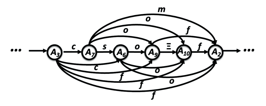
We define an interval-based network (network for short) to represent a complex activity containing the temporal relationships between intervals. A node represents the -th interval (i.e. ) in a complex activity instance, while a directed link represents the relation between two intervals (i.e. and ), where ( is the cardinality of the set ). Note a link always starts from a node with a smaller index than its arrival node. Each link involves one and only one relation . Figure 2 illustrates the corresponding networks of a complex activity.


The temporal relations on links shall be globally consistent in any interval-based network. Given any two relations on links and , respectively, the relation on link must follow the transitivity properties as shown in Figure 3. For example, suppose meets and starts , is certainly meets . However, if starts and is finished by , there are three possible relations between and , that is, before, meet and overlap. We formally use to denote such composition operation following the transitivity properties. We say a network is consistent such that for any triplet of links , and in the network.
It is clear that a network can characterize one possible style of a complex activity with diverse combinations of atomic actions and their interval relations, as illustrated in Figure 2. From another point of view, a complex activity can be instantiated by sampling atomic actions and relations assigned to their associated nodes and links in a network following certain probabilities. In this way, a recognition model built on such networks is able to handle uncertainty in complex activity recognition. In addition, multiple occurrences of the same atomic action can appear in the same network but in different nodes (i.e. intervals). To this end, we present the probabilistic generative model IBGN where these networks can be constructed following the styles of the complex activities of interests under uncertainty. We shall also consider the IBGN model to construct networks with variable sizes of nodes and arbitrary structures. Note in our approach, for each type of complex activities we would learn one such dedicated IBGN model.
III Our IBGN Model
For any complex activity type (), denote the corresponding subset of instances, where each element is an instance of the -th type of complex activity In IBGN, the generative process of constructing an interval-based network for describing the observed instance consists of two parts, node generation and link generation, which are described below.
III-A Node Generation
In our IBGN model, we consider generating a network where each node is associated with an atomic action in a probabilistic manner. We also require our model to be capable of generating variable numbers of nodes and handling multiple occurrences of the same atomic action in our network, as summarized in Table I.
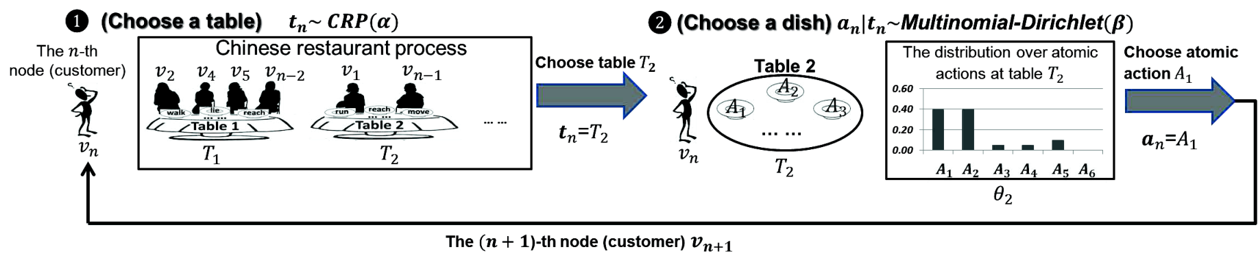
To accomplish these tasks, we first extend the process of the CRPs to make it available in our IBGN model. Originally, a CRP is analogous to a stochastic process of choosing tables for customers in a Chinese restaurant. In a nutshell, suppose there are an infinite number of tables . The first customer () always selects the first table; Any other customer () randomly selects an occupied table or an unoccupied empty table with a certain probability.
We continue this process by serving dishes right after each customer is seated at a table. Assume there are a finite number of dishes and an infinite number of cuisines. Each table is associated with a cuisine that dishes are served with a unique probability distribution. Any customer sitting at a table randomly selects a dish with the probability relating to its corresponding cuisine.
In our model, a network contains a group of customers where each customer is analogous to a node while a dish is analogous to an atomic action type. Suppose customers from the same group prefer similar cuisines, which is analogous to a complex activity of interest, and are more likely to sit at the same tables. Formally, denote the variables of tables, and the variables of atomic actions 22 2 Whenever possible, we would use bold lowercase letters such as , to represent variables, and uppercase letters such as and to represent generic values of these variables.. To construct a network , and are the table and the atomic action (dish) assigned to the node (customer) (). The generative process operates as follows. The -th node selects a table that is drawn from the following distribution:
| (1) |
where is the number of existing nodes occupied at table (), with , . is a tuning hyperparameter. It is worth mentioning that the distribution over table assignments in CRP is invariant and exchangeable under permutation according to de Finetti’s Theorem [28]. After is assigned with a table , an atomic action (dish) is chosen from the table by:
where is a hyperparameter. Note is the parameter vector of a multinomial distribution at table . Figure 4 presents a cartoon explanation of this node generation process of our IBGN model.


Since we would obtain one dedicated IBGN model for each complex activity, a complex activity is now characterized as a unique set of distributions over atomic actions, i.e. . As illustrated in Figure 5, the two different complex activities offensive play and defensive play are associated with two distinct sets of tables with their own distributions over atomic actions. It suggests that our IBGN modeling approach is capable of differentiating the underlying characteristics associated with atomic actions from different complex activity categories.
III-B Link Generation
Once each node (interval) is assigned to an atomic action, links and their associated relations are to be generated next. It is important to ensure consistency of the resulting relations over all links. Formally, given two relations and on the links and (), respectively, the interval relation on link shall follow the transitivity properties listed in Figure 3. It is straightforward to verify that the set is closed under the composition operation. As a result, by applying the transitivity table, for any composition there exists only possible transitive relations in Figure 6, denoted as . In other words, any composition of two consecutive relations satisfies .
To construct a globally consistent network, the relations on every triangle in a network must also be consistent. Namely, for any triplet of nodes , and , if there exist three links , , and , they need to satisfy the transitive relation . As such, we define the interval relation constraint variable as follows:
Definition 1.
Give an arbitrary interval-based network , the interval relation constraint for a link () is
In link generation, our IBGN model follows the rule that any relation can only be drawn from . We have proved that a network constructed under this rule is globally consistent and complete, with proofs relegated to the Appendix A.
Theorem 1.
(Network Consistency and Completeness)
A network constructed by obeying the interval relation constraints is always temporally consistent, and any possible combination of relations in can be constructed through our IBGN model.
Now, we are ready to assign relations to links. Suppose , and (, ), a relation on link is chosen from a distribution over all possible relations in as follows:
where is the parameter vector of the multinomial distribution associated with the triplet . Note that for an interval relation constraint containing only one relation (i.e. -), the probability of choosing that relation is always one.
It is also important to notice that the quality of the network structure plays an extremely important role in activity modeling. In our previous work [17], two variants with fixed network structures are considered: chain-based network as in Figure 7(a), where only the links between two neighbouring nodes are constructed in networks; fully-connected network as in Figure 7(b), where all pairwise links are constructed in networks. In fact, they are two special cases of our IBGN model. In chain-based networks, only a set of links are generated, with () representing the link of two neighboring nodes . Any interval relation constraint in chain-based networks equals to , and thus such networks are inherently consistent because no inconsistent triangle exists. However crucial relations may be missing in this model. On the other side of the spectrum, we have fully-connected networks, where all possible pairwise links are considered. Any in fully-connected networks equals to . When fitting the IBGN model, it is possible to increase the likelihood by adding links, but doing so may result in overfitting. Instead of prefixing the network structures, in this work we relax the assumption of a structure being either fully-connected or chain-based, and consider learning an optimal structure (i.e. to decide which links should exist in the network) from data. This allows the IBGN model to handle temporal consistency for arbitrary network structures, as presented in Figure 7(c).


III-C The Generative Process
For each dataset containing a particular complex activity , our model assumes the whole generative process including node generation and link generation in Algorithm 1. Notice that the optimal network structure would be learned from with details to be elaborated in section IV-A. The structure demonstrates whether a link needs to be generated in the network. For example, to construct the network for a certain complex activity instance , the link from to is involved in if and only if obeys the structure of , denoted by .
The joint distribution of variables , , and , is given by:
| (2) |
The total number of variables , , and are , and , respectively. It is worth noting that we often set , due to the fact that given a training dataset a number of tables are occupied at most.
IV IBGN Learning
In what follows we focus on how to learn the network structure and the parameter vectors and from the training data for a particular complex activity .
IV-A Learning Network Structure
Instead of configuring a network with chain-based or fully-connected links, we would like to learn an network structure in IBGN according to a score function that best matches the training data , i.e., learning from empirical data on which links to select in our constructed networks.
An IBGN model is built over a collection of variables for table assignments, for atomic-action assignments and for relation assignments. In detail, for a specific instance with , its corresponding network involves variables , , , . To consider a general network structure, we first introduce a null interval to make every instance in having the same number of intervals. A null interval is defined as such that its associated atomic action is null and its temporal relation with any other intervals is null. In other words, null can be viewed as a special atomic action class. For any instance of size , null intervals are appended at the rear of the instance. In this way, every instance has the same number of intervals. Correspondingly, any IBGN has a total number of possible random variables, with possible variables for tables , possible variables for atomic actions , possible variables for interval relations and possible variables for interval relation constraints . An exemplar IBGN model can be described in Figure 8, where each is associated with variables and , and each is associated with variable and , with .
To this end, our IBGN structure learning problem is defined as to find a such that the score of given is maximum.
Next, we employ structure constraints to translate the IBGN model to a corresponding problem in Bayesian networks.
Definition 2.
Given an IBGN model , its corresponding Bayesian network is defined as a directed bipartite graph where , with the structure constraints such that
where denotes the number of distinct elements of .
A node in () maps to the variable in , while a node in () maps to the variable in . That is, and . Notice that a null is introduced to represent the absence of a node or a relation in an instance of (constraint (2)), and thus there are possible atomic-action assignments for a node in and possible relation assignments for a node in . Moreover, any node in has no parent, and any node in has either being connected to the nodes and in or not being connected to any node (constraint (3)). That means a link exists in if and only if its corresponding node in has . The structure of associated with the variables is illustrated in Figure 9.
Now, the problem of determining whether a link should exist in IBGN is converted to the problem of finding a set of links with the maximal score under the above constraints. In particular, we consider the Bayesian Information Criterion () as the score function, which addresses the overfitting issue by introducing a penalty term in the structure, as proved in the Appendix B:
| (3) |
where is a constant. denotes the parents of the -th node in and , which is the number of possible instantiations of the parent set of the -th node. In fact, . For example, suppose be the -th node in and . If the links and exist in (i.e. ), then the node has two parents (i.e. ) whose number of categories is , and thus ; otherwise, . In addition, is the parameter vector such that , where and denotes that the -th node in is assigned with the -th element and its parent nodes are assigned with the -th element (i.e. an instantiation of its parent set ), respectively; indicates how many instances of contain both and . Note that any node has eight elements (i.e. ). At this stage, several techniques can be employed to learn the structure of efficiently [5, 10, 16]. After finding the best structure , a link is in if and only if .
IV-B Learning Parameters
We first estimate the parameters for node generation. Since the variable is latent for each node in our generative process, we shall approximately estimate the posterior distribution on by Gibbs sampling. Formally, we marginalize the joint probability in Eq.(2) and derive the posterior probability of latent variable being assigned to the table () as follows:
where is the count that nodes have been assigned to the atomic action type at the table , and is the count of nodes in that has been assigned to the table . refer to the atomic action assignments for nodes . is the count of occupied tables with . The suffix of means the count that does not include the current assignment of table for the node . is the tuning parameter for the -th table selection during CRP; is the Dirichlet prior for the -th atomic action conditioned on the -th table. We provide the detailed derivations of the Gibbs sampling in Appendix C. By sampling the latent tables following the above distribution, the distributions of () can be estimated as
Normally, the hyperparameters and are set as fixed values before the execution of a Gibbs sampler. In our IBGN model, and involve a number of and prior parameters, respectively. As they are unfortunately unknown beforehand, it is difficult to manually encode each parameter to proper values. As a result, we need to instead learn each hyperparameter to obtain reasonable results. The adoption of Gibbs sampling enables us to seamlessly incorporate the tuning of these hyperparameters as presented in Algorithm 2.
The stop condition may be that a predefined max iterations has been reached or that an estimation function converges to a given threshold. To update the hyperparameters and , a convergent method proposed by Minka [19] is used as follows:
where is digamma function, and the superscript indicates the sample generated by the Gibbs sampler at the -th iteration.
Next, we estimate the parameters for link generation. It can be seen that the probability distribution of variable relies on the triplet only (where , and ), and thus we can learn these parameters by maximum likelihood estimate method. In our IBGN model, given a triplet , the conditional probability distribution on is a multinomial over all possible relations in . Then, the likelihood of the parameter for with respect to is:
| (4) |
By applying a Lagrange multiplier to ensure , maximum likelihood estimate for is
| (5) |
where is the number of links are labeled with the -th relation in , with , , and . Note the trivial cases of for as each of them contains only one element as indicated in Figure 6.
Now, by integrating out the latent variable with all the parameters derived above, the probability of the occurrence of a new instance given the -th type of complex activity is estimated below
| (6) |
where and are the sets of atomic actions and their relations in the new instance, respectively, and indicate only these links obeying the structure of are counted. To predict which type of complex activity a new instance belongs to, we simply evaluate the posterior probabilities over each of the possible types of complex activities as
| (7) |
V Experiments
Experiments are carried out on three benchmark datasets as well as our in-house dataset on recognizing complex hand activities. In addition to the proposed approach IBGN, two variants with fixed network structures are also considered: One is IBGN-C for chain-based structures, where only the links between two neighbouring nodes in networks are constructed; The other one is IBGN-F for fully-connected structures, where all pairwise links in networks are constructed. Several well-established models are employed as the comparison methods, which include IHMM [20], dynamic Bayesian network (DBN) [12] and ITBN [31], where IHMM and DBN are implemented on our own, and ITBN is obtained from the authors. All internal parameters are tuned for best performance for a fair comparison. The standard evaluation metric of accuracy is used, which is computed as the proportion of correct predictions.
Experimental Set-Ups
The Raftery and Lewis diagnostic tool [24] is employed to detect the convergence of the Gibbs sampler (Algorithm 2) for the IBGN family. It has been observed that overall we have a short burn-in period, which suggests the Markov chain samples are mixing well. Thus and are set to the averaged counts of their first samples after convergence. In addition, we utilize the branch-and-bound algorithm [5] for constraints-based structure learning. This approach can strongly reduce the time and memory costs for learning Bayesian network structures based on the BIC score function (Eq. (3)) without losing global optimality guarantees. Besides, to avoid the division-by-zero issue in practice (i.e. in Eq. (5)), we instead use by introducing a small smoothing constant () in the following experiments.
Time Complexity Analysis
The time complexities of IBGN-C and IBGN-F are for training each complex activity category, where is the number of iterations executed in Algorithm 2. IBGN has an extra time complexity of for structure learning, where . On the other hand, the time complexities of the IBGN family at the testing stage are the same, which is for a single test instance.
V-A Experiments on Three Existing Benchmark Datasets
Datasets and Preprocessing
The three publicly-available complex activity recognition datasets collected from different types of cameras and sensors are considered, as summarized in Table. II. We employ these datasets in our evaluation due to their distinctive properties: The OSUPEL dataset [3] can be used to evaluate the case where only a handful of atomic action types and simple relations are recorded; Opportunity [25] is challenging as it contains a large number of atomic action types and also involves intricate interval relations in instances; CAD14 [15] represents the datasets having relatively larger number of complex activity categories.
| OSUPEL | Opportunity | CAD14 | |
|---|---|---|---|
| Application type | Basketball play | Daily living | Composable activities |
| Recording devices | one ordinary camera | 72 on-body sensors of 10 modalities | one RGB-D camera |
| E.g. of atomic actions | shoot, jump, dribble, etc. | sit, open door, wash cup, etc. | clap, talk phone, walk, etc. |
| E.g. of complex activities | two offensive play types | relax, cleanup, coffee time, early morning, sandwich time | talk and drink, walk while clapping, talk and pick up, etc. |
| No. of atomic action types | 6 | 211 | 26 |
| No. of complex activity types | 2 | 5 | 16 |
| No. of instances | 72 | 125 | 693 |
| No. of intervals per instance | 2-5 | 1-78 | 3-11 |
To recognize atomic actions in each dataset, we adopt the methods developed in their respective corresponding work. That is, we employed the dynamic Bayesian network models that are used to model and recognize each atomic action including shoot, jump, dribble and so on for OSUPEL [31]. Similarly, for CAD14 [15] we adopted the hierarchical discriminative model to recognize atomic action such as clap, talk phone and so on through an discriminative pose dictionary. For the sensor-based Opportunity dataset, we utilized the activity recognition chain system (ARC) [4] to recognize atomic action recognition from sensors. It is worth mentioning that we can also recognize null type of complex activity by labeling the intervals that are not annotated to any activities in the datasets.
Comparison under an Ideal Condition
First of all, the competing models are evaluated under the condition that all intervals are correctly detected. Table III displays the averaged accuracy results over 5-fold cross-validations, where the proposed IBGN family clearly outperforms other methods with a big margin on all three datasets. The reason is that IBGNs engage the rich interval relations among atomic actions. Although ITBN can also encode relations, it however fails with the multiple occurrences of the same atomic actions or when inconsistent relations existing among training instances. As a considerable amount of multiple occurrences of the same atomic actions and inconsistent temporal relations exist in CAD14, ITBN performs the worst. It can also be seen that IBGN-F with fully-connected relations performs better than IBGN-C on the Opportunity and CAD14 datasets where relations are intricate. However, IBGN-F might be overfitted when relations are simple, e.g. the OSUPEL dataset. Overall IBGN outperforms its two variants by its ability to adaptively learn network structures from data, where fixed structures might face the issue of either overfitting or underfitting.
| IHMM | DBN | ITBN | IBGN-C | IBGN-F | IBGN | |
| OSUPEL | 0.53 | 0.58 | 0.69 | 0.79 | 0.76 | 0.81 |
| Opportunity | 0.74 | 0.83 | 0.88 | 0.98 | 0.96 | 0.98 |
| CAD14 | 0.93 | 0.95 | 0.51 | 0.97 | 0.98 | 0.98 |
Robustness Tests under Atomic-Level Errors
In practice the accuracy of atomic action recognition will significantly affect complex activity recognition results. To evaluate the performance robustness, we also compare the competing models under atomic action recognition errors. First, it is important to check whether our model is robust under label perturbations of atomic-action-level (or atomic-level for short). To show this, we synthetically perturb the atomic-level predictions. Figure 10 reports the comparison results on Opportunity under two common atomic-level errors. It can be seen that IBGNs are more robust to misdetection errors where atomic actions are not detected or are falsely recognized as another actions. We perturbed the true labels with error rates ranging from 10-30 percents to simulate synthetic misdetection errors. Similarly, we also perturbed the start and end time of intervals with noises of 10-30 percents to simulate duration-detection errors where interval durations are falsely detected. It is also clear that IBGNs outperform other competing models under duration-detection errors.
In addition, we report the evaluated performances under real detected errors caused by the ARC system for atomic-level recognition. We chose three classifiers for atomic action recognition from the ARC system, i.e. kNN, SVM and DT. Features such as mean, variance, correlation and so on are selected by setting a time-sliced window of 1s. After classification, each interval is assigned to an atomic action type. As shown in Figure 10, the models which can manage interval relations are relatively more robust to the atomic-level errors than other models, such as ITBN and IBGNs. Moreover, it is evident that IBGNs are noticeably more robust than ITBN with around 15% – 87% performance boost. IBGN performs the best among its family because it is more capable of handling the structural variability in complex activities than the other two variants, which may avoid more noise existing in training and testing information. Note similar conclusions are also obtained on the OSUPEL and CAD14 datasets.
V-B Our Complex Hand Activity Dataset
Data Collection
We propose a new complex activity dataset on depth camera-based complex hand activities on performing American Sign Language (ASL). It is an ongoing effort, and at the moment it contains 3,480 annotated instances, which is already about 5-fold larger than existing ones. As illustrated in Fig. 11, complex activities in our dataset are defined as selected ASL hand-actions. There are 20 atomic actions, which are defined as the states of individual fingers, either straight or bent. It is important to realize that in a complex activity, there could be multiple occurrences of the same atomic action, as is also exemplified in Fig. 11(f) where an action A2 appears twice in the sub-network.



Sixteen subjects participate in the data collection, with various factors being taken into consideration to add to the data diversities. Subjects of different genders, ages groups, races are present in the dataset. The male to female ratio is 12 to 4, races ratio is 14 to 2 and participants’ ages span from around 15 to 40. For each subject, the depth image sequences are recorded with a front-mount SoftKinetic camera while performing designated complex activities in office settings, with a frame-rate of 25 FPS, image size of 320240, and hand-camera distance of around 0.6-1m. In total, the dataset contains 19 ASL hand-action complex activities, with each having 145-290 instances collected among all subjects. Each of the instance is comprised of 5-17 atomic action intervals. The 19 ASL hand-actions are air, alphabets, bank, bus, gallon, high school, how much, ketchup, lab, leg, lady, quiz, refrigerator, several, sink, stepmother, teaspoon, throw, xray.
Atomic Hand Action Detection
To detect atomic-level hand-actions, we make use of the existing hand pose estimation system [30] with a postprocessing step to map joint location prediction outputs to the bent/straight states of fingers. To evaluate performance of the interval-level atomic action detection results, we follow the common practice and use the intersection-over-union of intervals with a 50 threshold to identify a hit/false alarm/missing, respectively. Finally F1 score is used based on the obtained precision and recall values. Note here the finger bent states are considered as foreground intervals.
Robustness Tests under Atomic-Level Errors
We first evaluate the performance on simulated synthetic misdetection errors and duration-detection errors. From Fig. 12, we observe that overall IBGN is notably more robust than other approaches, meanwhile IHMM consistently produces the worst results. Our model is relatively robust in the presence of atomic-level errors.


Now we are ready to show the performance of our model when working with our atomic-level predictor as mentioned previously. Overall our atomic-level predictor achieves F1 score of 0.724. Table IV summarizes the final accuracy comparisons of the six competing approaches based on our atomic-level predictor vs. the atomic-level ground-truth labels on our hand-action dataset. It is not surprising that in both scenarios IBGN again significantly outperforms the rest approaches. It is worth noting that taking into account the challenging task of atomic-level hand pose estimation on its own, the gap in performances of vs. on predicting over 19 complex activity categories is reasonably, which is also certainly one thing we should improve over in the future.
| IHMM | DBN | ITBN | IBGN-C | IBGN-F | IBGN |
| with real atomic-level prediction | |||||
| 0.43 | 0.51 | 0.54 | 0.49 | 0.55 | 0.58 |
| with atomic-level ground-truth (ideal situation) | |||||
| 0.67 | 0.81 | 0.77 | 0.82 | 0.84 | 0.86 |
Fig. 13 presents the confusion matrix of IBGN working with our atomic-level predictor. We observe that our system is able to recognize the ASL words such as xray, alphabets and quiz very well. At the same time, several ASL words turn to be difficult to deal with, with accuracy under 50%. This may mainly due to the relatively low accuracy of the atomic-level predictor we are using on the particular atomic actions.
VI Conclusion
We present an interval-based Bayesian generative network approach to account for the latent structures of complex activities by constructing probabilistic interval-based networks with temporal dependencies in complex activity recognition. In particular, the Bayesian framework and the novel application of Chinese restaurant process (CRP) of our IBGN model enable us to explicitly capture inherit structural variability in each of the complex activities. In addition, we make publicly available a new complex hand activity dataset dedicated to the purpose of complex activity recognition, which contains around an-order-of-magnitude larger number of annotated instances. Experimental results suggest our proposed model outperforms existing state-of-the-arts by a large margin in a range of well-known testbeds as well as our new dataset. It is also shown that our approach is rather robust to the errors introduced by the low-level atomic action predictions from raw signals. As part of future work, we are considering relaxing the assumption that the IBGN models share the same structure for representing multiple instances of the same complex activity, and will instead learn more flexible structures for each class of complex activities by introducing latent structure variables that decide whether a link should exist in an instance. Also, we will continue the finalization of our hand-action dataset, improving the atomic-level atomic action prediction method, as well as attempting toward the establishment of standardized comparisons on exiting systems.
VII Acknowledgments
This research was supported in part by grant CQU903005203326 from the Fundamental Research Funds for the Central Universities in China, grants R-252-000-473-133 and R-252-000-473-750 from the National University of Singapore, and A*STAR JCO grants 15302FG149 and 1431AFG120.
Appendix A Proofs of Theorem 1
We first prove that the composition operation on the interval relation union set satisfies the associative law. The set of all the unions is denoted by .
Definition 3.
(Composition Product of Two Relation Sets)
The composition product of two sets of interval relations , i.e. and , where any , is defined as
.
Lemma 2.
(Associative Law on Composition)
Proof.
Let , and , where any . Then, and Since the composition on the seven interval relation set satisfies the associative law that is both left and right associative, the associative law also holds on , which is closed under the composition operation, i.e. , for any . So, we have . ∎
Lemma 3.
(Path Consistency)
Given an IBGN , if for any , then for any path in , .
Proof.
For any path in , we have and , then . Iteratively, we finally have . ∎
Proof.
(Consistency)
Lemma 3 indicates that if any in the network satisfies the transitivity properties, then any path in the network also satisfies the transitivity properties. Hence, the entire network generated through our construction is consistent.
(Completeness)
(by contradiction)
Suppose there exists one interval relations that cannot be generated through our construction, i.e. , which means there exists at least one () that . This contradicts the fact that the network is consistent. Besides, any possible relation in can be generated between two neighboring nodes. That is to say, any possible triangle that is consistent can be generated by our model. ∎
Appendix B Proof of
Proof.
The corresponding variable dependence in the IBGN model is shown as follows:
|
|
According to our definition of the generative process, the structure between and (marked as blue line), the structure among and the structure between and (marked as blue dotted line) are fixed. We only need to learn the structure between and .
In effect, the structure without and and their associated links (blue dotted lines) is equivalent to the Bayesian structure defined in Definition 2, where and (constraint (1)). The number of categories of any atomic action variable () is , including the null atomic action. Similarly, the number of categories of any relation variable () is 8, including the null relation (constraint (2)). Given a training dataset , for any instance and its corresponding network , if , then and . Moreover, any atomic action variable has no parent, and any relation variable has either two parents or zero parents (constraint (3)). That is, a link exists in if and only if both and are connected with in .
Formally, let where , , and . denotes the parents of and , where is the number of categories of . In particular, we have
where is a constant. Suppose the corresponding variable of the node equals , we have
Since the structure between and , the structure among and the structure between and are fixed, the number of parents of a node are fixed. Then, we have
Also, let be the entire vector of parameters such that , where and denotes that is assigned with the -th element and its parent is assigned with the -th element in , respectively; indicates how many instances of contain both and . Here, we split the parameter vector into three parts: , , and are the parameter vectors associated with , , and , respectively. Given a training dataset , we have
Similarly, in , any node has no parent, and thus . We split the parameter vector into two parts: and are the parameter vectors associated with and , respectively. Then, we have
Let
Given a dataset , the parameter vectors , , , can be estimated to maximize their respective logarithmic equations regardless of the network structures. Similarly, for the parameters such that and , they can also be estimated invariably under arbitrary network structures. Therefore, is constant. Then we have
∎
Appendix C Conditional distribution for Gibbs sampling
Since the probability of conditioned on is Dirichlet-multinomial distribution, we can write out the integration formulae:
The total number of tables cannot exceed the maximum network size .
The probability of conditioned on its previous tables follows CRP . We adopt the technique introduced by Sudderth [27] to sample the -th table in as follows
where is the number of time the previous nodes in are assigned to the table , and is the Kronecker delta function that
and denotes a previously empty table.
Now we derive the conditional probability of each variable of the -th table in assigned to the table by Gibbs sampling as follows:
References
- [1] Aggarwal, J., Ryoo, M.: Human activity analysis: A review. ACM Computing Surveys 43(3), 16 (2011)
- [2] Allen, J.: Maintaining knowledge about temporal intervals. ACM Communications 26(11), 832–843 (1983)
- [3] Brendel, W., Fern, A., Todorovic, S.: Probabilistic event logic for interval-based event recognition. In: CVPR (2011)
- [4] Bulling, A., Blanke, U., Schiele, B.: A tutorial on human activity recognition using body-worn inertial sensors. ACM Computing Surveys 46(3), 33 (2014)
- [5] Campos, C.D., Ji, Q.: Efficient structure learning of Bayesian networks using constraints. JMLR 12, 663–689 (2011)
- [6] Chen, L., Hoey, J., Nugent, C., Cook, D., Yu, Z.: Sensor-based activity recognition. Systems, Man, and Cybernetics, Part C: Applications and Reviews, IEEE Transactions on 42(6), 790–808 (2012)
- [7] Cook, D.J., Krishnan, N.C., Rashidi, P.: Activity discovery and activity recognition: a new partnership. IEEE Transactions on Cybernetics 43(3), 820–828 (2013)
- [8] Devanne, M., Wannous, H., Berretti, S., Pala, P.: 3-d human action recognition by shape analysis of motion trajectories on riemannian manifold. IEEE Transactions on Cybernetics 45(7), 1023–1029 (2014)
- [9] Dubba, K.S.R., Cohn, A.G., Hogg, D.C., Bhatt, M., Dylla, F.: Learning relational event models from video. Journal of Artificial Intelligence Research 53(1), 41–90 (2015)
- [10] Fan, X., Yuan, C.: An improved lower bound for Bayesian network structure learning. In: AAAI (2015)
- [11] Helaoui, R., Niepert, M., Stuckenschmidt, H.: Recognizing interleaved and concurrent activities: A statistical-relational approach. In: IEEE International Conference on Pervasive Computing and Communications (2011)
- [12] Hu, D., Yang, Q.: CIGAR: Concurrent and interleaving goal and activity recognition. In: AAAI (2008)
- [13] Kim, E., Helal, S., Cook, D.: Human activity recognition and pattern discovery. IEEE Pervasive Computing 9(1), 48–53 (2010)
- [14] Lara, O.D., Labrador, M.: A survey on human activity recognition using wearable sensors. IEEE Communications Surveys & Tutorials 15(3), 1192–1209 (2013)
- [15] Lillo, I., Soto, A., Niebles, J.: Discriminative hierarchical modeling of spatio-temporally composable human activities. In: CVPR (2014)
- [16] Liu, A.A., Su, Y.T., Jia, P.P., Gao, Z., Hao, T., Yang, Z.X.: Multipe/single-view human action recognition via part-induced multitask structural learning. IEEE Transactions on Cybernetics 45(6), 1194–1208 (2015)
- [17] Liu, L., Cheng, L., Liu, Y., Jia, Y., Rosenblum, D.: Recognizing complex activities by a probabilistic interval-based model. In: AAAI (2016)
- [18] Liu, L., Wang, S., Peng, Y., Huang, Z., Liu, M., Hu, B.: Mining intricate temporal rules for recognizing complex activities of daily living under uncertainty. Pattern Recognition 60, 1015–1028 (2016)
- [19] Minka, T.: Estimating a Dirichlet distribution (2000)
- [20] Modayil, J., Bai, T., Kautz, H.: Improving the recognition of interleaved activities. In: Int. Conf. Ubiquitous computing (2008)
- [21] Oliver, N., Horvitz, E.: A comparison of hmms and dynamic Bayesian networks for recognizing office activities. In: User Modeling, pp. 199–209 (2005)
- [22] Pinhanez, C.S.: Representation and recognition of action in interactive spaces. Ph.D. thesis, MIT (1999)
- [23] Pitman, J.: Combinatorial stochastic processes. Tech. rep., Technical Report 621, Dept. Statistics, UC Berkeley (2002)
- [24] Raftery, A.E., Lewis, S.: How many iterations in the Gibbs sampler. Bayesian statistics 4(2), 763–773 (1992)
- [25] Roggen, D., Calatroni, A., Rossi, M., Holleczek, T., et al.: Collecting complex activity datasets in highly rich networked sensor environments. In: Int. Conf. Networked Sensing Systems (2010)
- [26] Ryoo, M., Aggarwal, J.: Semantic representation and recognition of continued and recursive human activities. Int. j. of compt. vision 82(1), 1–24 (2009)
- [27] Sudderth, E.B.: Graphical models for visual object recognition and tracking. Ph.D. thesis, MIT (2006)
- [28] Teh, Y.W.: Dirichlet process. In: Encyclopedia of machine learning, pp. 280–287 (2011)
- [29] Veeraraghavan, H., Papanikolopoulos, N., Schrater, P.: Learning dynamic event descriptions in image sequences. In: IEEE Conference on Computer Vision & Pattern Recognition, pp. 1–6 (2007)
- [30] Xu, C., Nanjappa, A., Zhang, X., Cheng, L.: Estimate hand poses efficiently from single depth images. International Journal of Computer Vision 116(1), 21–45 (2016)
- [31] Zhang, Y., Zhang, Y., Swears, E., Larios, N., Wang, Z., Ji, Q.: Modeling temporal interactions with interval temporal Bayesian networks for complex activity recognition. IEEE Transactions on Pattern Analysis and Machine Intelligence 35(10), 2468–2483 (2013)