A Hierarchical Image Matting Model for Blood Vessel Segmentation in Fundus imagesThanks: This work was supported by the National Natural Foundation of Guangdong Province, Integrated Platform of Evolutionary Intelligence and Robot, support no.(2015KGJHZ015). Zhun Fan, Jiewei Lu and Wenji Li are with the Guangdong Provincial Key Laboratory of Digital Signal and Image Processing, College of Engineering, Shantou University, Shan’tou 515063, China (email: zfan, 12jwlu1, liwj@stu.edu.cn). Caimin Wei is with the Department of Mathematics, Shantou University, Shan’tou 515063, China (email: cmwei@stu.edu.cn). Han Huang is with the School of Software Engineering, South China University of Technology, Guang’zhou 510006, China (email: hhan@scut.edu.cn). Xinye Cai is with the College of Computer Science and Technology, Nanjing University of Aeronautics and Astronautics, Jiang’su 210016, China (email:xinye@nuaa.edu.cn). Xinjian Chen is with the Medical Image Processing and Analysis Lab, School of Electronics and Information Engineering, Soochow University, Su’zhou 215006, China (email: xjchen@suda.edu.cn).
Abstract
In this paper, a hierarchical image matting model is proposed to extract blood vessels from fundus images. More specifically, a hierarchical strategy utilizing the continuity and extendibility of retinal blood vessels is integrated into the image matting model for blood vessel segmentation. Normally the matting models require the user specified trimap, which separates the input image into three regions manually: the foreground, background and unknown regions. However, since creating a user specified trimap is a tedious and time-consuming task, region features of blood vessels are used to generate the trimap automatically in this paper. The proposed model has low computational complexity and outperforms many other state-of-art supervised and unsupervised methods in terms of accuracy, which achieves a vessel segmentation accuracy of , and in an average time of , and on images from three publicly available fundus image datasets DRIVE, STARE, and CHASE_DB1, respectively.
Index Terms:
Image matting, hierarchical strategy, fundus, trimap, region features, segmentation, vessel.I Introduction
Retinal blood vessels generally show a coarse to fine centrifugal distribution and appear as a wire mesh-like structure or tree-like structure. Their morphological features, such as length, width and branching, play an important role in diagnosis, screening, early detection and treatment of various cardiovascular and ophthalmologic diseases such as stroke, vein occlusions, diabetes and arteriosclerosis [1]. The analysis of morphological features of retinal blood vessels can facilitate a timely detection and treatment of a disease when it is still in its early stage. Moreover, the analysis of retinal blood vessels can assist in evaluation of retinal image registration [2], the relationship between vessel tortuosity and hypertensive retinopathy [3], retinopathy of prematurity [4], arteriolar narrowing [5], mosaic synthesis [6], biometric identification [7], foveal avascular region detection [8] and computer-assisted laser surgery [1]. Since cardiovascular and ophthalmologic diseases have a serious impact on human’s life, the analysis of retinal blood vessels becomes more and more important. It is of great significance in many clinical applications to reveal important information of systemic diseases and support diagnosis and treatment. As a result, the requirement of vessel analysis system grows rapidly in which the segmentation of retinal blood vessels is the first and one of the most crucial steps.
The segmentation of retinal blood vessels has been a heavily researched area in recent years [9]. Broadly speaking, existing algorithms can be divided into supervised and unsupervised methods. In supervised methods, a number of different features are extracted from fundus images, and applied to train the effective classifiers with the purpose of extracting retinal blood vessels. In [10], Staal et al. extracts 27 features for each image pixel with ridge profiles, and performs feature selection by using sequential forward selection method to pick those pixels that result in better segmentation performance by a K-Nearest Neighbor (KNN) classifier. Soares et al. [11] introduces a feature-based Bayesian classifier with Gaussian mixtures for vessel segmentation, which uses the intensity information and Gabor wavelet transform responses to build a 7-D feature vector for each pixel. In [12], Lupascu et al. utilizes an AdaBoost classifier and a 41-D feature vector which includes information on the local intensity structure, spatial properties, and geometry at multiple scales. Marin et al. [13] constructs a 7-D vector composed of gray-level and moment invariants-based features, and then trains a neural network (NN) for pixel classification. Roychowdhury et al.[14] extracts the major vessel from the fundus images and uses a Gaussian Mixture Model classifier for vessel segmentation with a set of 8 features, which are extracted based on pixel neighborhood and first and second-order gradient images. In [15], Liskowski et al. employs a deep neural network to extract vessel pixels from fundus images. In unsupervised methods, the researchers try to find inherent properties of retinal blood vessels that can be applied to extract vessel pixels from fundus images. The unsupervised methods can be further divided into multiscale approaches, matched filtering, vessel tracking, mathematical morphology and model based methods [9]. The multiscale approach introduced by [16] develops a vessel enhancement filter with the analysis of multiscale second order local structure of an image (Hessian), and obtains a vesselness measure by using the eigenvalues of the Hessian. The matched filtering method described by [17] employs different threshold probes to extract blood vessels from matched filter response images. In [18], the methodology based on vessel tracking applies a wave propagation and traceback mechanism to label each pixel the likelihood of belonging to vessels in angiography images. The mathematical morphology with the extraction of vessel centerlines [19] is also developed to find the morphological characteristics of retinal blood vessels. Model based methods generally use geometric deformable models [20], parametric deformable models [21], vessel profile models [22] and active contour models [23] for blood vessel segmentation.


Image matting refers to the problem of accurately extracting a foreground object from an input image. Generally image matting includes two main steps. The first step is generating a user specified trimap. An example of a user specified trimap is shown in Fig.1(b). The trimap is a hand-drawn segmented image, which separates the input image into three regions: foreground (shown in white), background (shown in black) and unknown (shown in gray). The second step is applying the image matting model to extract the pixels belonging to the foreground object from the unknown regions, based on the samples of foreground and background pixels marked by the user. An exemplary result achieved by [24] is shown in Fig.1(c). Image matting is very useful in many important applications, such as image (or video) segmentation, image editing, video production, new view synthesis, and film making. To the best of our knowledge, image matting has never been employed before to extract blood vessels from fundus images. The major reason is that for retinal blood vessel segmentation, generating a user specified trimap is a tedious and time-consuming task. In other words, it is not appropriate to create a trimap manually for retinal blood vessel segmentation. In addition, a normal image matting model needs to be designed carefully to improve the performance of blood vessel segmentation. In order to overcome these problems, region features of blood vessels are applied to generate the trimap automatically. Then a hierarchical image matting model is proposed to extract the pixels of blood vessel from the unknown regions. More specifically, a hierarchical strategy utilizing the continuity and extendibility of retinal blood vessels is integrated into the image matting model for blood vessel segmentation. The proposed model is evaluated on three public available datasets DRIVE, STARE, and CHASE_DB1, which have been widely used by other researchers to develop their own methods. The vessel segmentation performance demonstrates the efficiency and effectiveness of the proposed hierarchical image matting model.
The rest of this paper is structured as follows: Section II provides some background knowledge of image matting, and a brief introduction of vessel enhancement filters applied in our work. Section III details the process of generating the trimap of a fundus image automatically, and the proposed hierarchical image matting model. Section IV introduces the public available datasets and the commonly used evaluation metrics. Section V presents the experimental results. In Section VI, the discussion and conclusion are given.
II Related Work
In this section, we will first review some background knowledge of image matting, and then briefly introduce vessel enhancement filters used in our work.
II-A Image Matting
As aforementioned, image matting aims to accurately extract the foreground given a trimap of an image. Specifically, the input image is modeled as a linear combination of a foreground image and a background image :
| (1) |
where , called alpha matte, is the opacity of the foreground. ranges from to . If is constrained to be either or , then the matting problem becomes the segmentation problem, where each pixel belongs to either foreground or background.
After obtaining the user specified trimap, to infer the alpha matte in the unknown regions, Chuang et al. [25] uses sets of Gaussian distribution to model the color distributions of the foreground and background images, and estimates the optimal alpha value with a maximum-likelihood criterion. In [26], Levin et al. derives an effective cost function from the assumption that the foreground and background colors are locally smooth, and employs this function to find the optimal alpha matte. Zheng et al. [24] proposes a local learning based approach and a global learning based approach to perform image matting. In [27], Kaiming et al. solves a large kernel matting Laplacian, and achieves a fast matting algorithm. In [28], Shahrian and Rajan analyze the texture and color features of the image, and optimize an objective function containing the color and texture components to choose the best foreground and background pair for image matting. Shahrian et al. [29] expands the sampling range of foreground and background regions, and collects a representative set of samples to estimate the alpha matte. In [30], Cho et al. presents an image matting method to extract alpha mattes across sub-images of a light field image.
II-B Vessel Enhancement filters
Vessel enhancement filters plays an important role in retinal blood vessel segmentation [9]. Here two effective filters [31, 32] used in our work are introduced.
II-B1 Morphologically Reconstructed Filter
Morphologically reconstructed filter is an effective tool for blood vessel enhancement [31]. For each input fundus image , the green channel image is extracted firstly since has the best vessel-background contrast [13]. Then the morphological top-hat transformation is performed:
| (2) |
where is the complement image of , represents the top-hat transformed image, is a structuring element for morphological opening , and specifies the angle (in degrees) of the structuring element. The structuring element is of 1-pixel width and 21-pixels length, which approximately fits the diameter of the biggest vessels in the fundus images [31]. Since the morphological top-hat transformation transformation given in Equation (2) can only brighten blood vessels in one direction, the sum of top-hat transformation along each direction is performed in order to enhance the whole vessel image:
| (3) |
where represents the enhanced vessel image using morphologically reconstructed filter, ”A” is the set of angles of the structuring element and defined as .
II-B2 Isotropic Undecimated Wavelet Filter
The isotropic undecimated wavelet filter has been used for blood vessel segmentation, and has a good performance on vessel enhancement [32]. Applied to a signal ( is the input green channel image), scaling coefficients are computed by convolution with a filter firstly:
| (4) |
where is derived form the cubic B-spline, is the upsampled filter obtained by inserting zeros between each pair of adjacent coefficients of . Wavelet coefficients are the difference between two adjacent sets of scaling coefficients, i.e.,
| (5) |
Reconstruction of the original signal from all wavelet coefficients and the final set of scaling coefficients is straightforward, and requires only addition. The final enhanced vessel image is depicted as follows:
| (6) |
where represents the enhanced vessel image using isotropic undecimated wavelet filter. In blood vessel segmentation, wavelet scales: are selected according to [32].


III Methodology
In this section, the process of generating the trimap of an input fundus image automatically is introduced, followed by detailing the proposed hierarchical image matting model.
| Threshold values | ||||
|---|---|---|---|---|
| Default values | ||||
| Recommended Ranges |
III-A Trimap Generation
Region features of blood vessels have been used for blood vessel segmentation and performed well on segmentation accuracy and computational efficiency [33]. In this paper, region features of blood vessels are applied to generate the trimap of the input fundus image automatically. The definitions of regions features are given as follows:
- •
Area indicates the actual number of pixels in the region.
- •
Bounding Box specifies the smallest rectangle containing the region. An example for the illustration of bounding box is shown in Fig.2(b).
- •
Extent is the ratio of pixels in the region to pixels in the total bounding box.
- •
VRatio is the ratio of the length to the width of the bounding box.
- •
Convex Hull specifies the smallest convex polygon that can contain the region. An example for the illustration of convex hull is shown in Fig.2(c).
- •
Solidity is the ratio of pixels in the region to pixels in the total convex hull.
The default threshold values of region features:Extent, VRatio, Solidity and their recommended ranges used in this work are reported in Table I. and are two threshold values of Extent features used in this work; is the threshold value of feature; is the threshold value of feature. For feature, two threshold values: and are used in this work. , called the internal factor, is calculated as , where is approximately the diameter of the biggest vessels in fundus images[31], and are the height and width of the fundus image.
The proposed model is not sensitive to above mentioned region features. In other words, these region features can be selected in a relatively large range without sacrificing the performance. In Section V(D)-”Sensitivity analysis of threshold values of region features”, empirical study is conducted to verify the insensitivity of the proposed model to the threshold values of region features.
Creating the trimap of the input fundus image includes two main steps: 1) Image Segmentation and 2) Vessel Skeleton Extraction. The process of trimap generation is given in Fig.3.


III-A1 Image Segmentation
The goal of image segmentation is to divide the input image into three regions: the vessel (foreground), background and unknown regions. Firstly the enhanced vessel image is segmented into three regions: the background regions (), unknown regions () and preliminary vessel regions ()
| (7) |
where and restrict the unknown region as thin as possible in order to achieve the better matting result [34, 28]. In order to remove the noise regions in , the regions with in are extracted firstly (). Then regions in whose && && are abandoned, resulting in the denoised preliminary vessel regions . An example of image segmentation is shown in Fig.4.


III-A2 Vessel Skeleton Extraction
Vessel Skeleton Extraction aims to further distinguish the unknown regions and provide more information on blood vessels. In Section V(B)-”Vessel Segmentation Performance”, the effectiveness of vessel skeleton extraction will be presented. Firstly, a binary image is obtained by global thresholding the enhanced vessel image .
| (8) |

where , is set as . Then is divided into three regions according to the feature:
| (9) |
In vessel skeleton extraction, the regions in are preserved while the regions in are abandoned. Then the regions in with && are preserved as . Finally skeleton extraction [35] is performed on the combined regions of and in order to obtain the skeleton of blood vessels . An example of vessel skeleton extraction is shown in Fig.5.
After performing image segmentation and vessel skeleton extraction, the trimap of the input fundus image is generated (as shown in Fig.7(b)), which is composed of the background regions (), unknown regions () and vessel (or foreground) regions ().


III-B Hierarchical Image Matting Model
Hierarchical image matting model is proposed to label the pixels in the unknown regions as vessels or background in an incremental way. Specifically, after stratifying the pixels in unknown regions (called unknown pixels) into hierarchies by a hierarchical strategy, let indicates the th unknown pixel in the th hierarchy, the segmented vessel image is modeled as follows:
| (10) |
where indicates the correlation function (depicted in Equation (13)). The implementation of the hierarchical image matting model consists of two main steps:
- Step 1
-
Stratifying the unknown pixels: Stratify pixels in the unknown regions into different hierarchies.
- Step 2
-
Hierarchical update: Assign new labels ( or ) to pixels in each hierarchy.
The pseudocode of implementing this model is given in Algorithm 1.
| Algorithm 1: Implementing the hierarchical image matting model |
|---|
| Input: Trimap composed of , , |
| Output: The segmented vessel image |
| Step 1: Stratifying the unknown pixels: a) For , set , where is the number of unknown pixels in , is the distance between the th unknown pixel and the closest vessel pixel in , is the set of . b) Sort the unknown pixels in in an ascending order according to the distances , cluster the pixels with the same distance into one hierarchy, stratify the pixels into hierarchies and denote them as an hierarchical order set: , , where is the number of unknown pixels in the th hierarchy . Step 2: Hierarchical Update |
| For , do |
| For , do a) Compute the correlations (Defined in Equation (13)) between and its neighboring labelled pixels(vessel pixels and background pixels) included in a grid. b) Choose the labelled pixel with the closest correlation, and assign its label ( or ) to . end for |
| end for |
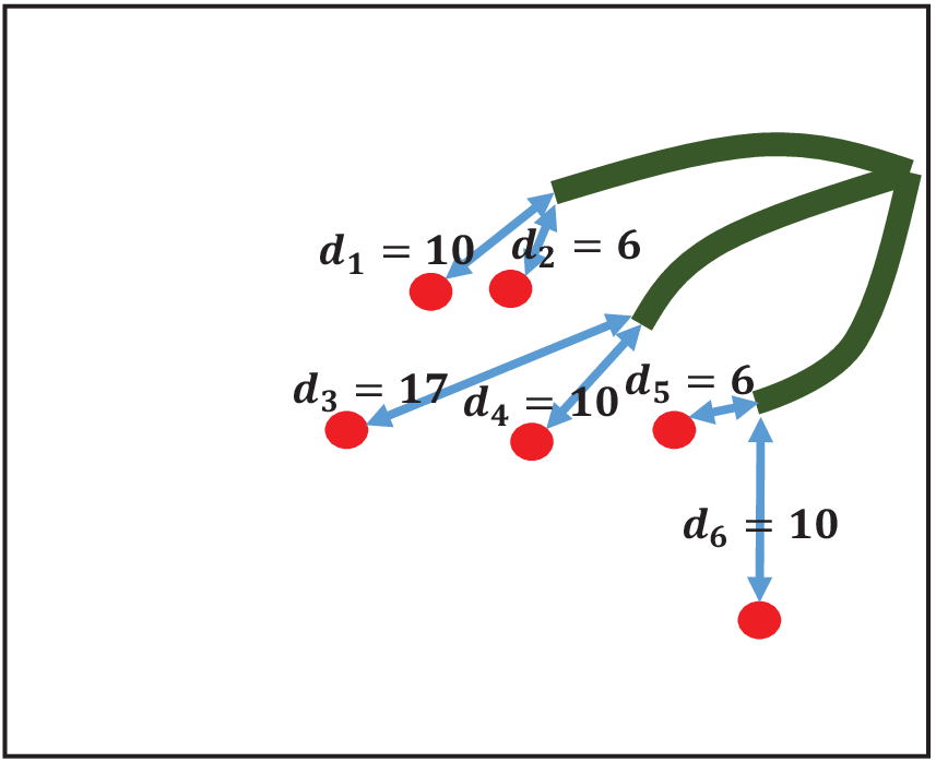
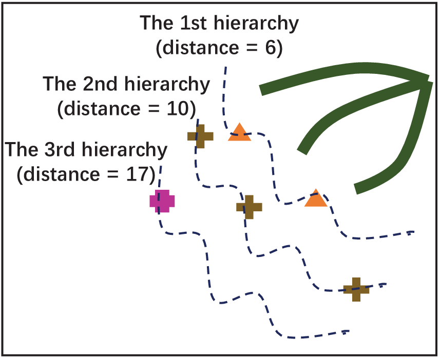
Stratifying the unknown pixels: In this stage, the unknown pixels are stratified into different hierarchies. For the th unknown pixel in , its distances with all vessel pixels in are calculated first. Then the closest distance is chosen and assigned to the th unknown pixel. After that, the unknown pixels are stratified into different hierarchies according to the closest distances. The first hierarchy has the lowest value of the closet distance while the last hierarchy has the highest value of the closet distance. The unknown pixels reside in low hierarchy suggests that they are close to blood vessels; The unknown pixels stay in high hierarchy indicates that they are far away from blood vessels. An example to illustrate the process of stratifying the unknown pixels is shown in Fig.6.


Correlation Function: In step 2 of Algorithm 1, given an unknown pixel and its neighboring labelled pixel , a color cost function is defined to describe the fitness of and first:
| (11) |
where and are intensity level of and in . A spatial cost function is further defined:
| (12) |
where and are the spatial coordinates of and . The terms and are the maximum and minimum distance of the unknown pixel to the labelled pixel . The normalization factors and ensure that is independent from the absolute distance.
Our final correlation function is a combination of the color fitness and the spatial distance:
| (13) |
where is a weight to trade off the color fitness and spatial distance. is set as in our experiment. Intuitively, a small indicates that the labelled pixel has a close correlation with the unknown pixel.
Hierarchical Update: After performing initialization with the hierarchical strategy, in each hierarchy, the correlations between each unknown pixel and its neighboring labelled pixels (vessel pixels and background pixels) included in a grid are computed. Then the labelled pixel with the closest correlation is chosen, and its label is assigned to the unknown pixel. After all unknown pixels in one hierarchy are updated, they are used for the update of the next hierarchy. The unknown pixels are updated from the first hierarchy to the last hierarchy. An example to illustrate the process of updating unknown pixels in one hierarchy is shown in Fig.8.
III-C Postprocessing
Since some non-vessel regions may still exist in the final segmented vessel image , the regions whose && && in are abandoned to remove these non-vessel regions.
IV Datasets and Evaluation Metrics
In this section, three publicly available datasets are introduced. These datasets have been widely used by researchers to test their own vessel segmentation algorithms. Then some commonly used evaluation metrics are presented, which are also utilized in our experiment and to compare the proposed method with other state-of-art methods.
IV-A Datasets
The proposed model is evaluated on three standard datasets: DRIVE [10], STARE [17] and CHASE_DB1 [31].
DRIVE11 1 http://www.isi.uu.nl/Research/Databases/DRIVE/ consists of 40 fundus images obtained from a screening program in the Netherlands. These images are captured by a Canon CR5 non-mydriatic 3-CCD camera at field of view (FOV), and the size of each image is of pixels. The DRIVE dataset is divided into two sets: a training set (DRIVE Training) and a test set (DRIVE Test) each containing 20 fundus images. The training set is annotated by two observers; The test set is annotated by two independent human observers.
STARE22 2 http://www.ces.clemson.edu/ ahoover/stare/ consists of 20 fundus images. These images are captured by a TopCon TRV-50 fundus camera at FOV, and the size of each image is of pixels. Ten images contain pathology while the other ten images are normal. The STARE dataset is annotated by two independent observers.
CHASE_DB133 3 https://blogs.kingston.ac.uk/retinal/chasedb1/ consists of 28 fundus images acquired from multiethnic school children. These images are captured by a hand-held Nidek NM-200-D fundus camera at FOV, and the size of each image is of pixels. The CHASE_DB1 is annotated by two independent observers.
For the DRIVE, STARE and CHASE_DB1 datasets, the manual segmentations of the first observer are used in this work, which is a common choice for these datasets [36, 15, 9, 23].
| Test Datasets | DRIVE | STARE | ||||||||||
|---|---|---|---|---|---|---|---|---|---|---|---|---|
| Methods | Acc | AUC | Se | Sp | Time | Acc | AUC | Se | Sp | Time | System | |
| Supervised Methods | ||||||||||||
| Staal et.al[10] | 0.944 | - | - | - | 15min | 0.952 | - | - | - | 15min | 1.0 GHz, 1-GB RAM | |
| Soares et.al[11] | 0.946 | - | - | - | 3min | 0.948 | - | - | - | 3min | 2.17 GHz, 1-GB RAM | |
| Lupascu et.al[12] | 0.959 | - | 0.720 | - | - | - | - | - | - | - | - | |
| Marin et.al[13] | 0.945 | 0.843 | 0.706 | 0.980 | 90s | 0.952 | 0.838 | 0.694 | 0.982 | 90s | 2.13 GHz, 2-GB RAM | |
| Roychowdhury et.al[14] | 0.952 | 0.844 | 0.725 | 0.962 | 3.11s | 0.951 | 0.873 | 0.772 | 0.973 | 6.7s | 2.6 GHz, 2-GB RAM | |
| Liskowski et.al[15] | 0.954 | 0.881 | 0.781 | 0.981 | - | 0.973 | 0.921 | 0.855 | 0.986 | - | NVIDIA GTX Tian GPU | |
| Unsupervised Methods | ||||||||||||
| Hoover et.al[17] | - | - | - | - | - | 0.928 | 0.730 | 0.650 | 0.810 | 5min | Sun SPARCstation 20 | |
| Mendonca et.al[19] | 0.945 | 0.855 | 0.734 | 0.976 | 2.5min | 0.944 | 0.836 | 0.699 | 0.973 | 3min | 3.2 GHz, 980-MB RAM | |
| Lam et.al[37] | - | - | - | - | - | 0.947 | - | - | - | 8min | 1.83 GHz, 2-GB RAM | |
| Al-Diri et.al[21] | - | - | 0.728 | 0.955 | 11min | - | - | 0.752 | 0.968 | - | 1.2 GHz | |
| Lam and Yan et.al[22] | 0.947 | - | - | - | 13min | 0.957 | - | - | - | 13min | 1.83 GHz, 2-GB RAM | |
| Perez et.al[38] | 0.925 | 0.806 | 0.644 | 0.967 | 2min | 0.926 | 0.857 | 0.769 | 0.944 | 2min | Parallel Cluster | |
| Miri et.al[39] | 0.943 | 0.846 | 0.715 | 0.976 | 50s | - | - | - | - | - | 3 GHz, 1-GB RAM | |
| Budai et.al[40] | 0.957 | 0.816 | 0.644 | 0.987 | - | 0.938 | 0.781 | 0.580 | 0.982 | - | 2.3 GHz, 4-GB RAM | |
| Nguyen et.al[41] | 0.941 | - | - | - | 2.5s | 0.932 | - | - | - | 2.5s | 2.4 GHz, 2-GB RAM | |
| Yitian et.al[23] | 0.954 | 0.862 | 0.742 | 0.982 | - | 0.956 | 0.874 | 0.780 | 0.978 | - | 3.1 GHz, 8-GB RAM | |
| Annunziata et.al[36] | - | - | - | - | - | 0.956 | 0.849 | 0.713 | 0.984 | 25s | 1.9 GHz, 6-GB RAM | |
| Orlando et.al[42] | - | 0.879 | 0.790 | 0.968 | - | - | 0.871 | 0.768 | 0.974 | - | 2.9 GHz, 64-GB RAM | |
| Proposed | 0.960 | 0.858 | 0.736 | 0.981 | 10.72s | 0.957 | 0.880 | 0.791 | 0.970 | 15.74s | 2.5 GHz, 4-GB RAM | |
IV-B Evaluation Metrics
In the process of retinal vessel segmentation, each pixel is classified as vessels or background, thereby resulting in four events: two correct (true) classifications and two incorrect (false) classifications, which are defined in Table III.
| Vessel present | vessel absent | |
|---|---|---|
| vessel detected | True Positive (TP) | False Positive (FP) |
| vessel not detected | False Negative (FN) | True Negative(TN) |
In order to evaluate the performance of the vessel segmentation algorithms, three commonly used metrics are applied.
Sensitivity () reflects the algorithm’s ability of detecting vessel pixels while Specificity () is a measure of the algorithm’s effectiveness in identifying background pixels. Accuracy () is a global measure of classification performance combing both and . The performance of the vessel segmentation method is also measured by the area under a receiver operating characteristic () curve (). The conventional is calculated from a number of operating points, and normally used to evaluate the balanced data classification problem. However, in practice the researchers need to select an operating point to compare their method with other methods. Also blood vessel segmentation is an unbalanced data classification problem, in which there are much fewer vessel pixels than the background pixels. In order to evaluate the performance of blood vessel segmentation properly, [43, 23] is applied to indicate the overall performance of blood vessel segmentation, which is suitable to describe the overall performance of imbalanced data classification problem and specifically for the case when only one operating point is used. The segmentation time required per image in seconds for implementing the proposed segmentation algorithm in MATLAB on a Laptop with Intel Core i7 processor, 2.5GHz and 8GB RAM is also recorded.
| Dataset | Method | Acc | AUC | Se | Sp | Time(s) |
|---|---|---|---|---|---|---|
| DRIVE | Trimap (Treating the unknown regions as background regions) | 0.959 | 0.833 | 0.679 | 0.986 | 5.841 |
| Model without vessel skeleton extraction | 0.960 | 0.837 | 0.688 | 0.986 | 11.959 | |
| Proposed | 0.960 | 0.859 | 0.736 | 0.981 | 10.720 | |
| STARE | Trimap (Treating the unknown regions as background regions) | 0.958 | 0.853 | 0.728 | 0.977 | 7.741 |
| Model without vessel skeleton extraction | 0.959 | 0.862 | 0.748 | 0.976 | 16.563 | |
| Proposed | 0.957 | 0.881 | 0.791 | 0.970 | 15.740 | |
| CHASE_DB1 | Trimap (Treating the unknown regions as background regions) | 0.948 | 0.771 | 0.565 | 0.977 | 21.088 |
| Model without vessel skeleton extraction | 0.954 | 0.789 | 0.597 | 0.981 | 60.847 | |
| Proposed | 0.951 | 0.815 | 0.657 | 0.973 | 50.710 |


|
(a) (b)


|
(c) (d)
V Experiments and Results
In this section, four sets of experiments are performed with the purpose of evaluating the proposed hierarchical image matting model. In the first experiment, the segmentation performance of the proposed model was compared with other state-of-art methods. In the second experiment, the vessel segmentation performance of the proposed model was analyzed. In the third experiment, the proposed hierarchical image matting model was compared with image matting models. In the last experiment, the sensitivity analysis of threshold values of region features used in the work was given.
V-A Comparison with other methods
In this section, the proposed model is compared with other state-of-art methods on two most popular public datasets: DRIVE and STARE. The CHASE_DB1 dataset is not used here since it is relatively new and has relatively few results in the literature. The segmentation performance and computational complexity of the proposed model in comparison with other state-of-art methods on the DRIVE and STARE datasets are given in Table II. It can be observed that for the DRIVE dataset, the accuracy of the proposed model is the highest among all existing methods with , and . On the STARE dataset, the accuracy and of the proposed model are the highest among unsupervised methods with , . Although one supervised method [15] has the best performance on STARE dataset, the method is computationally more complex due to the use of deep neural networks, which may need retraining for new datasets. In addition, the proposed model has a low computational complexity compared with other segmentation methods.
V-B Vessel Segmentation Performance
The segmentation performance of the proposed model on three public available datasets is given in Table IV. It can be observed that the proposed model can achieve more than segmentation accuracy on the DRIVE, STARE and CHASE_DB1 datasets, with the highest accuracy score achieved in the DRIVE dataset. Some exemplary segmentation results are shown in Fig.9. When treating the unknown regions as background regions, AUC=0.833 of trimap is lower than the proposed model while Acc of trimap is similar to the proposed model. In addition, of trimap is lower than the proposed model. These observations show that trimap can already have good segmentation performance, which indicates that the selection of region features is very effective in segmenting blood vessels. From Table IV, it can be observed that the model with vessel skeleton extraction can achieve more than increase of and increase of compared with the model without vessel skeleton extraction while of the model with vessel skeleton extraction is similar to the model without vessel skeleton extraction, which demonstrates the effectiveness of vessel skeleton extraction.
V-C Comparison with image matting models
The effectiveness of the proposed model in blood vessel segmentation has been validated through previous experiments. In order to further verify the effectiveness of our model, the proposed model is compared with four other image matting models: Anat Model [26], Zheng Model [24], Shahrian Model [28] and Improving Model [29]. The segmemtation results of these models on the DRIVE, STARE, and CHASE_DB1 datasets are given in Table V. It can be observed that the proposed model outperforms other image matting models in terms of in the DRIVE, STARE and CHASE_DB1 datasets. Also the proposed model achieves the highest scores of in three datasets.
| Dataset | Model | Acc | AUC | Se | Sp | Time(s) |
|---|---|---|---|---|---|---|
| DRIVE | Anat Model | 0.958 | 0.862 | 0.746 | 0.978 | 10.036 |
| Zheng Model | 0.958 | 0.862 | 0.746 | 0.978 | 11.837 | |
| Shahrian Model | 0.921 | 0.903 | 0.881 | 0.925 | 120.552 | |
| Improving Model | 0.958 | 0.862 | 0.746 | 0.978 | 360.000 | |
| Proposed | 0.960 | 0.859 | 0.736 | 0.981 | 10.720 | |
| STARE | Anat Model | 0.944 | 0.839 | 0.714 | 0.964 | 11.376 |
| Zheng Model | 0.954 | 0.883 | 0.799 | 0.966 | 14.185 | |
| Shahrian Model | 0.912 | 0.906 | 0.899 | 0.913 | 145.860 | |
| Improving Model | 0.954 | 0.883 | 0.799 | 0.966 | 381.923 | |
| Proposed | 0.957 | 0.881 | 0.791 | 0.970 | 15.740 | |
| CHASE_DB1 | Anat Model | 0.944 | 0.820 | 0.675 | 0.964 | 29.047 |
| Zheng Model | 0.944 | 0.820 | 0.675 | 0.964 | 40.587 | |
| Shahrian Model | 0.918 | 0.858 | 0.790 | 0.927 | 340.899 | |
| Improving Model | 0.944 | 0.820 | 0.675 | 0.965 | 797.960 | |
| Proposed | 0.951 | 0.815 | 0.657 | 0.973 | 50.710 |
V-D Sensitivity analysis of threshold values of region features
The default threshold values of region features: , , , are used in our work. In order to demonstrate the insensitivity of the proposed model to these threshold values, the variations in by varying , , and are given in Fig.10.(a), (b), (c) and (d). From Fig.10, it can be observed that the proposed model can maintain high segmentation accuracy on the DRIVE, STARE and CHASE_DB1 datasets as varies in or varies in ; For and , the proposed model can maintain high segmentation accuracy as varies in or varies in . From the above observation, it can be seen that the proposed model is not sensitive to these threshold values of region features when they change in a relatively large range.


VI Conclusion
Image matting refers to the problem of accurately extracting a foreground object from an input image, which is very useful in many important applications. However, to the best of our knowledge, image matting has never been employed before to extract blood vessels from fundus image. The major reason is that for retinal blood vessel segmentation, generating a user specified trimap is a tedious and time-consuming task. In addition, a normal image matting model needs to be designed carefully to improve the performance of blood vessel segmentation. In order to overcome these problems, region features of blood vessels are applied to generate the trimap automatically. Then a hierarchical image matting model is proposed to extract the pixels of blood vessel from the unknown regions. More specifically, a hierarchical strategy utilizing the continuity and extendibility of retinal blood vessels is integrated into the image matting model for blood vessel segmentation.
The proposed model is very efficient and effective in blood vessel segmentation, which achieves a segmentation accuracy of , and on three public available datasets with an average time of , and , respectively. The experimental results show that it is a very competitive model compared with many other segmentation approaches, and has a low computational time.
References
- [1] J. J. Kanski and B. Bowling, Clinical Ophthalmology: A Systematic Approach. Elsevier Health Sciences, 2011.
- [2] F. Zana and J.-C. Klein, “A multimodal registration algorithm of eye fundus images using vessels detection and hough transform,” IEEE Transactions on Medical Imaging, vol. 18, no. 5, pp. 419–428, 1999.
- [3] M. Foracchia, E. Grisan, and A. Ruggeri, “Extraction and quantitative description of vessel features in hypertensive retinopathy fundus images,” in Book Abstracts 2nd International Workshop on Computer Assisted Fundus Image Analysis, vol. 6, 2001.
- [4] C. Heneghan, J. Flynn, M. O¡¯Keefe, and M. Cahill, “Characterization of changes in blood vessel width and tortuosity in retinopathy of prematurity using image analysis,” Medical Image Analysis, vol. 6, no. 4, pp. 407–429, 2002.
- [5] E. Grisan and A. Ruggeri, “A divide et impera strategy for automatic classification of retinal vessels into arteries and veins,” in Engineering in Medicine and Biology Society, 2003. Proceedings of The 25th Annual International Conference of The IEEE, vol. 1, 2003, pp. 890–893.
- [6] K. Fritzsche, A. Can, H. Shen, C. Tsai, J. Turner, H. Tanenbuam, C. Stewart, B. Roysam, J. Suri, and S. Laxminarayan, “Automated model based segmentation, tracing and analysis of retinal vasculature from digital fundus images,” State-of-The-Art Angiography, Applications and Plaque Imaging Using MR, CT, Ultrasound and X-rays, pp. 225–298, 2003.
- [7] C. Mariño, M. G. Penedo, M. Penas, M. J. Carreira, and F. Gonzalez, “Personal authentication using digital retinal images,” Pattern Analysis and Applications, vol. 9, no. 1, pp. 21–33, 2006.
- [8] A. Haddouche, M. Adel, M. Rasigni, J. Conrath, and S. Bourennane, “Detection of the foveal avascular zone on retinal angiograms using markov random fields,” Digital Signal Processing, vol. 20, no. 1, pp. 149–154, 2010.
- [9] M. M. Fraz, P. Remagnino, A. Hoppe, B. Uyyanonvara, A. R. Rudnicka, C. G. Owen, and S. A. Barman, “Blood vessel segmentation methodologies in retinal images–a survey,” Computer Methods and Programs In Biomedicine, vol. 108, no. 1, pp. 407–433, 2012.
- [10] J. Staal, M. D. Abràmoff, M. Niemeijer, M. A. Viergever, and B. van Ginneken, “Ridge-based vessel segmentation in color images of the retina,” IEEE Transactions on Medical Imaging, vol. 23, no. 4, pp. 501–509, 2004.
- [11] J. V. Soares, J. J. Leandro, R. M. Cesar, H. F. Jelinek, and M. J. Cree, “Retinal vessel segmentation using the 2-d gabor wavelet and supervised classification,” IEEE Transactions on Medical Imaging, vol. 25, no. 9, pp. 1214–1222, 2006.
- [12] C. A. Lupascu, D. Tegolo, and E. Trucco, “Fabc: Retinal vessel segmentation using adaboost,” IEEE Transactions on Information Technology in Biomedicine, vol. 14, no. 5, pp. 1267–1274, 2010.
- [13] D. Marín, A. Aquino, M. E. Gegúndez-Arias, and J. M. Bravo, “A new supervised method for blood vessel segmentation in retinal images by using gray-level and moment invariants-based features,” IEEE Transactions on Medical Imaging, vol. 30, no. 1, pp. 146–158, 2011.
- [14] S. Roychowdhury, D. D. Koozekanani, and K. K. Parhi, “Blood vessel segmentation of fundus images by major vessel extraction and subimage classification,” IEEE Journal of Biomedical and Health Informatics, vol. 19, no. 3, pp. 1118–1128, 2015.
- [15] P. Liskowski and K. Krawiec, “Segmenting retinal blood vessels with deep neural networks,” IEEE Transactions on Medical Imaging, vol. 35, pp. 1–1, 2016.
- [16] A. F. Frangi, W. J. Niessen, K. L. Vincken, and M. A. Viergever, “Multiscale vessel enhancement filtering,” in International Conference on Medical Image Computing and Computer-Assisted Intervention. Springer, 1998, pp. 130–137.
- [17] A. Hoover, V. Kouznetsova, and M. Goldbaum, “Locating blood vessels in retinal images by piecewise threshold probing of a matched filter response,” IEEE Transactions on Medical Imaging, vol. 19, no. 3, pp. 203–210, 2000.
- [18] F. K. Quek and C. Kirbas, “Vessel extraction in medical images by wave-propagation and traceback,” IEEE Transactions on Medical Imaging, vol. 20, no. 2, pp. 117–131, 2001.
- [19] A. M. Mendonca and A. Campilho, “Segmentation of retinal blood vessels by combining the detection of centerlines and morphological reconstruction,” IEEE Transactions on Medical Imaging, vol. 25, no. 9, pp. 1200–1213, 2006.
- [20] K. Sum and P. Y. Cheung, “Vessel extraction under non-uniform illumination: A level set approach,” IEEE Transactions on Biomedical Engineering, vol. 55, no. 1, pp. 358–360, 2008.
- [21] B. Al-Diri, A. Hunter, and D. Steel, “An active contour model for segmenting and measuring retinal vessels,” IEEE Transactions on Medical Imaging, vol. 28, no. 9, pp. 1488–1497, 2009.
- [22] B. S. Lam, Y. Gao, and A. W.-C. Liew, “General retinal vessel segmentation using regularization-based multiconcavity modeling,” IEEE Transactions on Medical Imaging, vol. 29, no. 7, pp. 1369–1381, 2010.
- [23] Y. Zhao, L. Rada, K. Chen, S. P. Harding, and Y. Zheng, “Automated vessel segmentation using infinite perimeter active contour model with hybrid region information with application to retinal images,” IEEE Transactions on Medical Imaging, vol. 34, no. 9, pp. 1797–1807, 2015.
- [24] Y. Zheng and C. Kambhamettu, “Learning based digital matting,” in Computer Vision and Pattern Recognition (CVPR), 2009 IEEE Conference on. IEEE, 2009, pp. 889–896.
- [25] Y.-Y. Chuang, B. Curless, D. H. Salesin, and R. Szeliski, “A bayesian approach to digital matting,” in Computer Vision and Pattern Recognition (CVPR), 2001 IEEE Conference on, vol. 2. IEEE, 2001, pp. II–II.
- [26] A. Levin, D. Lischinski, and Y. Weiss, “A closed-form solution to natural image matting,” IEEE Transactions on Pattern Analysis and Machine Intelligence, vol. 30, no. 2, pp. 228–242, 2008.
- [27] K. He, J. Sun, and X. Tang, “Fast matting using large kernel matting laplacian matrices,” in Computer Vision and Pattern Recognition (CVPR), 2010 IEEE Conference on. IEEE, 2010, pp. 2165–2172.
- [28] E. Shahrian and D. Rajan, “Weighted color and texture sample selection for image matting,” in Computer Vision and Pattern Recognition (CVPR), 2012 IEEE Conference on. IEEE, 2012, pp. 718–725.
- [29] E. Shahrian, D. Rajan, B. Price, and S. Cohen, “Improving image matting using comprehensive sampling sets,” in Computer Vision and Pattern Recognition (CVPR), 2013 IEEE Conference on, 2013, pp. 636–643.
- [30] D. Cho, S. Kim, and Y.-W. Tai, “Consistent matting for light field images,” in European Conference on Computer Vision. Springer, 2014, pp. 90–104.
- [31] M. M. Fraz, P. Remagnino, A. Hoppe, B. Uyyanonvara, A. R. Rudnicka, C. G. Owen, and S. A. Barman, “An ensemble classification-based approach applied to retinal blood vessel segmentation,” IEEE Transactions on Biomedical Engineering, vol. 59, no. 9, pp. 2538–2548, 2012.
- [32] P. Bankhead, C. N. Scholfield, J. G. McGeown, and T. M. Curtis, “Fast retinal vessel detection and measurement using wavelets and edge location refinement,” PloS One, vol. 7, no. 3, p. e32435, 2012.
- [33] Z. Fan, J. Lu, and Y. Rong, “Automated blood vessel segmentation of fundus images using region features of vessels,” in Computational Intelligence (SSCI), 2016 IEEE Symposium Series on. IEEE, 2016, pp. 1–6.
- [34] J. Wang and M. F. Cohen, “An iterative optimization approach for unified image segmentation and matting,” in Tenth IEEE International Conference on Computer Vision (ICCV’05) Volume 1, vol. 2. IEEE, 2005, pp. 936–943.
- [35] L. Lam, S.-W. Lee, and C. Y. Suen, “Thinning methodologies-a comprehensive survey,” IEEE Transactions on Pattern Analysis and Machine Intelligence, vol. 14, no. 9, pp. 869–885, 1992.
- [36] R. Annunziata, A. Garzelli, L. Ballerini, A. Mecocci, and E. Trucco, “Leveraging multiscale hessian-based enhancement with a novel exudate inpainting technique for retinal vessel segmentation,” IEEE Journal of Biomedical and Health Informatics, vol. 20, no. 4, pp. 1129–1138, 2016.
- [37] B. S. Y. Lam and H. Yan, “A novel vessel segmentation algorithm for pathological retina images based on the divergence of vector fields,” IEEE Transactions on Medical Imaging, vol. 27, no. 2, pp. 237–246, 2008.
- [38] M. A. Palomera-Pérez, M. E. Martinez-Perez, H. Benítez-Pérez, and J. L. Ortega-Arjona, “Parallel multiscale feature extraction and region growing: Application in retinal blood vessel detection,” IEEE Transactions on Information Technology in Biomedicine, vol. 14, no. 2, pp. 500–506, 2010.
- [39] M. S. Miri and A. Mahloojifar, “Retinal image analysis using curvelet transform and multistructure elements morphology by reconstruction,” IEEE Transactions on Biomedical Engineering, vol. 58, no. 5, pp. 1183–1192, 2011.
- [40] I. Section, “Robust vessel segmentation in fundus images,” International Journal of Biomedical Imaging, vol. 2013, no. 6, p. 154860, 2013.
- [41] U. T. Nguyen, A. Bhuiyan, L. A. Park, and K. Ramamohanarao, “An effective retinal blood vessel segmentation method using multi-scale line detection,” Pattern Recognition, vol. 46, no. 3, pp. 703–715, 2013.
- [42] J. I. Orlando, E. Prokofyeva, and M. B. Blaschko, “A discriminatively trained fully connected conditional random field model for blood vessel segmentation in fundus images,” IEEE Transactions on Biomedical Engineering, vol. 64, no. 1, pp. 16–27, 2017.
- [43] X. Hong, S. Chen, and C. J. Harris, “A kernel-based two-class classifier for imbalanced data sets,” IEEE Transactions on Neural Networks, vol. 18, no. 1, pp. 28–41, 2007.