Isotropic Layer Construction and Phase Diagram for Fracton Topological Phases

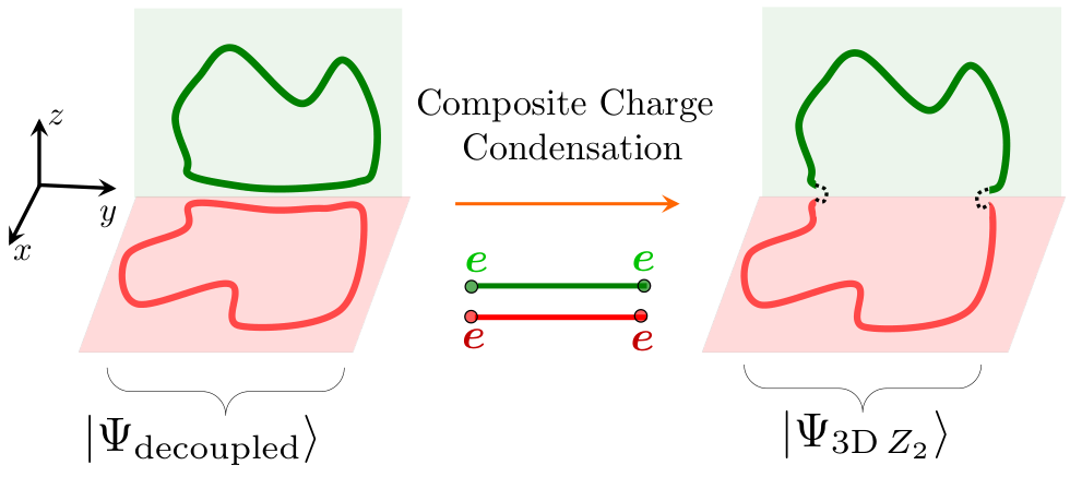
Starting from the decoupled phase, we now increase $h$, while keeping $J$ and $t$ fixed, which eventually leads to a $(3+1)$-dimensional $Z_{2}$ topological phase. Before demonstrating this explicitly with the microscopic Hamiltonian (3), we obtain intuition for this result by studying how the ground-state wavefunction changes as $h$ is increased. When acting on the decoupled toric codes, the operator $\sigma^{z}_{\boldsymbol{s}\boldsymbol{s}^{\prime}}\mu^{z}_{\boldsymbol{s}\boldsymbol{s}^{\prime}}$ creates four electric charge excitations in the orthogonal layers that meet at the link connecting sites $\boldsymbol{s}$ and $\boldsymbol{s}^{\prime}$, as shown in Fig. 3. Increasing $h$ leads to the condensation of this excitation, which we refer to as the composite electric charge.

Condensing the composite electric charge “glues” the planar electric charge loops in the wavefunction for the decoupled toric codes ($\ket{\Psi_{\mathrm{decoupled}}}$). As shown in Fig. 4, adding a composite electric charge has the effect of “cutting open” two electric charge loops in orthogonal layers that appear in a loop configuration in the state $\ket{\Psi_{\mathrm{decoupled}}}$. This “cut” loop configuration is to be interpreted as a single, three-dimensional loop of the emergent electric charge $A_{\boldsymbol{s}}^{(xy)}A_{\boldsymbol{s}}^{(yz)}A_{\boldsymbol{s}}^{(xz)}$, which remains well-defined in the condensed phase, and the resulting loop superposition is precisely the wavefunction for the 3D $Z_{2}$ topological phase. As we will soon show, composite charge condensation also has the effect of binding the 2D $Z_{2}$ fluxes into flux loops. In this way, the 3D electric charge inherits its bosonic self-statistics and $\pi$-mutual statistics with flux loops from the 2D $Z_{2}$ phase.

We now derive this result from the microscopic Hamiltonian (3). When $h\gg J$, $t$, we let $\sigma_{\boldsymbol{r}\boldsymbol{r}^{\prime}}^{z}\mu_{\boldsymbol{r}\boldsymbol{r}^{\prime}}^{z}=+1$ and define a single spin degree of freedom for every link of the cubic lattice as

In terms of this spin, we obtain an effective Hamiltonian in perturbation theory

where the coupling $\widetilde{J}\sim O(J^{3}/h^{2})$. Here, the operator

is precisely the six-spin operator that measures the $Z_{2}$ charge in a (3+1)-dimensional $Z_{2}$ topological phase, while

is the four-spin operator measuring the flux through plaquette $p$ on the cubic lattice. When $t=0$, the effective Hamiltonian $H_{\mathrm{eff}}^{(1)}$ is precisely that of the 3D toric code [31]. Furthermore, increasing $t$ eventually leads to condensation of the $Z_{2}$ flux loops, resulting in a trivial, confined phase. As advertised, the 2D $Z_{2}$ fluxes are confined, while a bound-state of the $Z_{2}$ fluxes survives as a topological excitation, which becomes the flux loop of the three-dimensional $Z_{2}$ topological phase. Condensing a composite excitation has led to the emergence of a new topological excitation whose mobility is restricted.

While composite charge condensation leads to three-dimensional $Z_{2}$ topological order, condensing a bound-state of the $Z_{2}$ fluxes in adjacent layers – a composite flux loop – yields the so-called “X-cube” fracton topological phase, as originally introduced and studied in Ref. [26] using an exactly solvable, commuting Hamiltonian. We first review the phenomenology of the X-cube fracton topological phase before demonstrating that this phase emerges within our layer construction. A detailed description of this fracton phase is provided in Ref. [26].

The spirit of our proposal motivates the construction of new, three-dimensional topological orders, by appropriately condensing “loop” objects in an array of two-dimensional topological phases. An extended discussion of new topological phases that may be built in this manner is the subject of forthcoming work [62]. Here, we discuss the simplest generalization of our construction, involving an array of two-dimensional $Z_{N}$ toric codes [14] in the same configuration as shown in Fig. 1, which gives rise to a $Z_{N}$ generalization of the X-cube model. After arranging the $Z_{N}$ toric codes in a three-dimensional array, each link of the three-dimensional cubic lattice now has two $Z_{N}$ qudit degrees of freedom, denoted $X_{\boldsymbol{r}\boldsymbol{r}^{\prime}}$, $Z_{\boldsymbol{r}\boldsymbol{r}^{\prime}}$ and $\widetilde{X}_{\boldsymbol{r}\boldsymbol{r}^{\prime}}$, $\widetilde{Z}_{\boldsymbol{r}\boldsymbol{r}^{\prime}}$ respectively, and satisfying the algebra $XZ=\omega ZX$, $\widetilde{X}\widetilde{Z}=\omega\widetilde{Z}\widetilde{X}$ with $\omega=e^{2\pi i/N}$. We now consider the Hamiltonian

where $H_{0}$ describes the de-coupled layers of $Z_{N}$ toric codes

with $A_{\boldsymbol{r}}^{(j)}$ and $B_{\boldsymbol{r}}^{(j)}$ the $Z_{N}$ charge and flux operators at site $\boldsymbol{r}$, for the toric code oriented along plane $j$, respectively. The layers are coupled through the interactions

Following our previous analysis, we consider the limit $h\gg J$, $t$, where we find that the ground-state exhibits 3D $Z_{N}$ topological order. In this limit, we may identify a single $Z_{N}$ degree of freedom on each link of the cubic lattice (with logical operators $\boldsymbol{X}$, $\boldsymbol{Z}$), and obtain the effective Hamiltonian $H_{\mathrm{toric}}^{\prime}-t\sum_{\boldsymbol{r}\boldsymbol{r}^{\prime}}[\boldsymbol{X}_{\boldsymbol{r}\boldsymbol{r}^{\prime}}+\mathrm{h.c.}]$ where $H_{\mathrm{toric}}^{\prime}$ is now the 3D $Z_{N}$ toric code Hamiltonian [61]. Alternatively, when $t\gg J$, $h$ so that we have condensed the “$Z_{N}$ composite flux loop”, we obtain the effective Hamiltonian

where

is the solvable Hamiltonian for the $Z_{N}$ generalization of the X-cube model. The microscopic form of the operators $\mathcal{O}_{c}$ and $A_{\boldsymbol{r}}^{(j)}$ are explicitly given in Fig. 7.

Since the operators $\mathcal{O}_{c}$ and $A_{\boldsymbol{r}}^{(j)}$ commute, the ground-state of (17) again satisfies $\mathcal{O}_{c}\ket{\Psi}=A_{\boldsymbol{r}}^{(j)}\ket{\Psi}=\ket{\Psi}$, and gapped excited states may be created by acting with straight Wilson line or flat membrane operators, in a straightforward generalization of the operators in the $Z_{2}$ X-cube model. Now however, the dimension-1 quasiparticles and fracton excitations carry a $Z_{N}$ electric and magnetic charge, respectively, which is inherited from the underlying 2D $Z_{N}$ toric codes. As a result, a pair of fractons which are mobile in a plane have bosonic self-statistics, but non-trivial mutual statistics $e^{i\theta_{pq}}$ with a dimension-1 quasiparticle of charge $q\in\{1,\ldots,N-1\}$ in its plane of motion. Here, the statistical angle $\theta_{pq}=2\pi pq/N$, where $p$ is the magnetic charge carried by the fracton excitation.

We begin from the top left corner of the phase diagram ($h\gg J$, $t$), where our system is in a 3D $Z_{N}$ topological phase. Increasing the strength of the coupling $t$ eventually leads to a condensation of $Z_{N}$ flux loops, and the associated phase transition is captured by the finite-temperature behavior of the 4D classical $Z_{N}$ lattice gauge theory with a “Wilsonian” imaginary time action $S_{W}[\theta]=\beta\widetilde{K}\sum_{p}\cos[(\Delta\times\theta)_{p}]$, where $\theta$ is a $Z_{N}$ variable defined on the links of the 4D cubic lattice, while $(\Delta\times\theta)_{p}$ is the lattice curl around plaquette $p$, and the sum is over all plaquettes on the 4D lattice.

When $N<5$, classical Monte Carlo studies [43, 44] have observed a direct, first-order phase transition between a disordered phase where the magnetic flux loops have condensed at high temperatures, to one where they remain energetically costly, with the expectation value of classical Wilson loop operators decaying as the exponential of the area of an enclosed region (“area-law”) and as their total length (“perimeter-law”), respectively, in the two phases. In our problem, these two phases correspond to a trivial loop condensate and a phase with $Z_{N}$ topological order, respectively, as indicated in the top portion of the phase diagram in Fig. 8a.

When $N$ is large ($N\geq 5$), three phases are observed in Monte Carlo studies of the classical 4D $Z_{N}$ lattice gauge theory [43, 44, 42]. This rich phase structure may be understood in a variety of ways. To begin, we recall that a similar phenomenon occurs in 2D classical, $Z_{k}$-symmetric spin models when $k$ is sufficiently large. In addition to a low-temperature symmetry-breaking phase and a disordered phase at high temperatures, there is an intermediate phase with algebraic correlations that resembles the low-temperature behavior of the XY model. The existence of this XY-like phase with an emergent global $U(1)$ symmetry may be motivated by recalling that in the classical 2D XY model, $Z_{k}$ anisotropy is a marginally irrelevant perturbation when $k\geq 4$ [37]. A more rigorous argument for the existence of this phase, even when the anisotropy is infinitely strong, is provided in Ref. [40].

A similar argument may be used for the presence of an intermediate phase with emergent $U(1)$ gauge symmetry in the phase diagram of 4D $Z_{N}$ lattice gauge theory in the large-$N$ limit [42, 40, 41]. Ref. [41] studied a Villain form of the 4D $Z_{N}$ gauge theory, which exhibits a discrete analog of the electric-magnetic self-duality of compact $U(1)$ gauge theory [39], and whose action may be re-written as that of Maxwell electrodynamics in the presence of both electric and magnetic charges. While the action exhibits only a $Z_{N}$ gauge symmetry, it was argued that both the electric and magnetic excitations are strongly suppressed near the self-dual point in the large-$N$ limit, so that the effective action is that of pure Maxwell electromagnetism. As a result, when $N\geq 5$, there is a “Coulomb phase” that is encountered in the top region of the phase diagram in Fig. 8b, with the $Z_{N}$ variable $\theta$ effectively behaving as the emergent $U(1)$ gauge field.

These three phases may be distinguished by the behavior of the gauge-invariant Wilson loop operator $W_{C}$, which creates a closed tube of electric flux, along with its (electric-magnetic) dual $\Gamma_{\widetilde{C}}$, which is a membrane-like operator that creates a closed magnetic flux loop along loop $\widetilde{C}$ on the dual lattice. In the deconfined phase of the $Z_{N}$ gauge theory, a large Wilson loop $W_{C}$ exhibits perimeter-law behavior while $\Gamma_{\widetilde{C}}$ has area-law behavior, while the opposite behavior occurs in the confined phase. In the intermediate phase, however, both charge and loop excitations are suppressed [41] and neither excitation has condensed. As a result, the Wilson loop operator $W_{C}$ must exhibit perimeter-law behavior [41]. Since this phase is self-dual under the electric-magnetic duality transformation, the same behavior holds for $\Gamma_{\widetilde{C}}$. As argued in Ref. [38], due to the non-trivial statistics of $Z_{N}$ charges and flux loops, perimeter-law behavior for both operators can only occur in the presence of a gapless gauge field, which is consistent with the emergence of a Coulomb phase.

It remains unclear whether the transition between the Coulomb and confined phases is continuous [45, 46] or weakly first-order [47, 48]. However, the transition between the deconfined phase of the $Z_{N}$ gauge theory and the Coulomb phase appears continuous in Monte Carlo studies [43, 44, 42]. Finally, as $N$ increases, the region of stability for the $Z_{N}$ topological phase shrinks, while the second transition from the Coulomb phase to the confined phase remains robust [43]. This is consistent with the expectation that the limit “$N\rightarrow+\infty$”, should somehow reproduce the phase diagram of the pure (3+1)-d compact $U(1)$ gauge theory.

We now study the bottom half of the phase diagrams shown in Fig. 8a & b. We first demonstrate that the transition from the decoupled layers of 2D toric codes to the X-cube fracton phase is dual to the confinement transition for the (3+1)-d $Z_{N}$ gauge theory, which is driven by the condensation of flux loops. This result is intuitively apparent from our “loop-gas” representation of the X-cube phase, which suggests that the transition from the decoupled layers must be driven by the condensation of a loop excitation. Physically, our duality transformation maps the closed composite flux loops in the ground-state of the X-cube phase into the closed electric flux loops in the ground-state of the $Z_{N}$ topological phase. We emphasize that this duality relates the bulk spectrum of two seemingly distinct physical systems, and provides relations between certain local operators on both sides.

We begin by explicitly implementing our lattice duality transformation on the Hamiltonian for the coupled $Z_{2}$ toric codes (3) when $h=0$, before discussing its consequences. In practice, our transformation is identical to the (2+1)-d Wegner duality that maps the transverse-field Ising model to the (2+1)-d $Z_{2}$ gauge theory [1], in each layer of our coupled system; as a result, the generalization of this duality for the $Z_{N}$ case is apparent from our following discussion. Recall that the Hamiltonian (3) for the coupled toric codes when $h=0$ is given by

We recognize that the 2D $Z_{2}$ charge operator $A_{\boldsymbol{r}}^{(j)}$ and the operator $\mathcal{O}_{\boldsymbol{r}}=B_{\boldsymbol{r}}^{(xy)}B_{\boldsymbol{r}}^{(yz)}B_{\boldsymbol{r}}^{(xz)}B_{\boldsymbol{r}+\hat{x}}^{(yz)}B_{\boldsymbol{r}+\hat{y}}^{(xz)}B_{\boldsymbol{r}+\hat{z}}^{(xy)}$, which is the product of six flux operators around an elementary cube, as in Eq. (11), commute with the Hamiltonian (18) and with each other $[\mathcal{O}_{\boldsymbol{r}},A_{\boldsymbol{r}^{\prime}}^{(j)}]=[A_{\boldsymbol{r}}^{(j)},H]=[\mathcal{O}_{\boldsymbol{r}},H]=0$. Therefore, we work in a restricted Hilbert space where

without loss of generality.

We now introduce a dual description of the transition from the decoupled theory ($t\ll J$) to the X-cube phase ($J\gg t$) that solves the first of these constraints, by introducing spins $(\eta)$ on the links of the dual cubic lattice. These spins are to be interpreted as measuring the flux through a plaquette in the decoupled toric code layers. We implement the dual representation by performing the replacements

where $\mathcal{B}_{\boldsymbol{r}\boldsymbol{s}}$ is a four-spin operator on a plaquette of the dual lattice pierced by the link $\langle\boldsymbol{r},\,\boldsymbol{s}\rangle$ as shown in Fig. 9.

The duality transformation preserves the algebra of local operators in (18), and naturally solves the constraint $A_{\boldsymbol{r}}^{(j)}\ket{\Psi}=\ket{\Psi}$. Furthermore, the dual description of the operator $\mathcal{O}_{\boldsymbol{r}}$ is given by

where $\mathcal{A}_{\boldsymbol{r}}$ is precisely the six-spin $Z_{2}$ charge operator which acts along a “star” configuration of the $\eta$ spins at each site of the dual cubic lattice. We therefore find that the dual Hamiltonian is precisely

supplemented by the $Z_{2}$ Gauss’s law constraint on the dual cubic lattice

which describes the confinement transition for a 3D $Z_{2}$ topological phase driven by the condensation of flux loops. As advertised, the lattice duality relates the $Z_{2}$ X-cube phase to the deconfined phase of (3+1)-d $Z_{2}$ gauge theory, while the decoupled toric code layers are dual to the trivial, confined phase.

Our duality transformation establishes that the bulk transition from the decoupled toric codes to the X-cube fracton phase is dual to flux loop condensation in the 3D $Z_{2}$ gauge theory, which is known to be a direct, first-order transition. The natural $Z_{N}$ generalization of this duality transformation leads us to conclude that along the $h=0$ line of the phase diagram (i) when $N<5$, there is a direct, first-order transition between the decoupled layers and the X-cube phase and (ii) when $N\geq 5$, there is an intermediate gapless phase for the layered system, which is dual to the Coulomb phase that emerges in the phase diagram of the (3+1)-d $Z_{N}$ gauge theory. From our duality transformation, it appears that this gapless “dual Coulomb” phase along the $h=0$ line of the phase diagram is characterized by an emergent $U(1)$ gauge symmetry, which should be generated by the natural generalization of the Gauss’s law condition $\mathcal{O}_{\boldsymbol{r}}=+1$ for the X-cube fracton phase. The $U(1)$ generalization of this condition may be read off from Fig. 7; if we consider an integer-valued “electric field” tensor $E_{ij}$ with vanishing diagonal components $E_{ii}=0$, and a conjugate gauge field $A_{ij}$, then this Gauss’s law takes the simple form

with $\Delta_{i}$, the lattice derivative along direction $i$, and summation performed over repeated indices.

The “higher-rank” compact $U(1)$ gauge theory [28, 49] defined by this Gauss’s law condition is equivalent to a generalized dimer model studied in Ref. [50], which was shown to be in a gapped phase with crystalline order due to the proliferation of topological defects in the gauge field configurations (i.e. “monopole” events). Due to this result, we believe that the dual Coulomb phase is unstable, and gives way to a gapped, topologically trivial phase with conventional long-range order when $h>0$. The $h=0$ line then corresponds to the fine-tuned limit where monopole events in the gauge field are suppressed. This conclusion is consistent with the fact that the perturbation $\sigma^{z}_{\boldsymbol{r}\boldsymbol{r}^{\prime}}\mu^{z}_{\boldsymbol{r}\boldsymbol{r}^{\prime}}$ corresponds to a highly non-local operator in terms of the dual $\eta$ spins, and with our expectation for the behavior of the phase diagram in the $N\rightarrow+\infty$ limit. The nature of the transitions between this trivial phase, the X-cube phase and the decoupled layers are unknown when $h>0$. When $h=0$, however, our duality mapping suggests that the phase transition from the X-cube phase to the dual Coulomb phase is dual to the transition between the deconfined phase of (3+1)-d $Z_{N}$ gauge theory and the ordinary Coulomb phase, which may be continuous [42, 43], though we are unaware of the continuum field theory that governs the properties of this transition.

We conclude this section by identifying the following order parameters

that distinguish the X-cube phase, the decoupled phase and the dual Coulomb phase along the line $h=0$. Here, $\Sigma$ is a two-dimensional region with area $A_{\Sigma}$ and perimeter $P_{\Sigma}$. The product appearing in the definition of $W_{\Sigma}$ is taken along the bonds perpendicular to the region $\Sigma$, and this operator may be thought of as inserting a composite flux loop along the boundary of $\Sigma$. Furthermore, ${\Gamma}_{\Sigma}$ is the product of the plaquette operators that measure the 2D $Z_{N}$ flux through the region $\Sigma$. Our notation is meant to emphasize that these operators are dual to the Wilson loop and membrane operators that distinguish the various phases of the $Z_{N}$ gauge theory. From our discussion in Sec. IIA, we determine that the operators $W_{\Sigma}$, $\Gamma_{\Sigma}$ exhibit the following behavior along the $h=0$ line, when the region $\Sigma$ is sufficiently large:

• •

  Decoupled Phase: $\langle{W}_{\Sigma}\rangle\sim e^{-\sigma A_{\Sigma}}$,    $\langle{\Gamma}_{\Sigma}\rangle\sim e^{-cP_{\Sigma}}$
  

• •

  Dual Coulomb Phase: $\langle{W}_{\Sigma}\rangle$, $\langle{\Gamma}_{\Sigma}\rangle\sim e^{-cP_{\Sigma}}$
  

• •

  X-cube Phase: $\langle{W}_{\Sigma}\rangle\sim e^{-cP_{\Sigma}}$,    $\langle{\Gamma}_{\Sigma}\rangle\sim e^{-\sigma A_{\Sigma}}$

The generic behavior of the confinement transition for the $Z_{N}$ X-cube fracton topological phase – by condensing the dimension-1 quasiparticle excitations – are not known. This transition occurs in the far right region of the phase diagrams in Fig. 8. Instead of studying this transition directly, however, we propose a solvable Hamiltonian that interpolates between the $Z_{2}$ X-cube fracton topological order and a confined phase in this section and determine that the transition is first-order within this model. It is unknown whether this captures the generic behavior of this transition, outside of the solvable model.

We construct a solvable projector model by placing spins $(\tau)$ on the links of a three-dimensional cubic lattice. Now, however, we consider the Hamiltonian

supplemented by the constraint

where $A_{\boldsymbol{r}}^{(j)}=\prod_{\boldsymbol{s}\in\mathrm{plane}_{j}(\boldsymbol{r})}\tau^{x}_{\boldsymbol{r}\boldsymbol{s}}$ is the four-spin operator in the X-cube model that is oriented in the $j$th plane, and measures the presence of a dimension-1 quasiparticle excitation at site $\boldsymbol{r}$. As before, the operator $\mathcal{O}_{\boldsymbol{r}}$ is the 12-spin $\tau^{z}$ operator as defined in Eq. (11) that measures the fracton “charge” at a cube $\mathcal{O}_{\boldsymbol{r}}=\prod_{\boldsymbol{s},\,\boldsymbol{r}^{\prime}\in\mathrm{cube}(\boldsymbol{r})}\tau^{z}_{\boldsymbol{r}^{\prime}\boldsymbol{s}}$. We observe that the Hamiltonian $\mathcal{H}$ exhibits both the $Z_{2}$ X-cube fracton phase ($h\ll J$) as well as a trivial confined phase ($h\gg J$). Furthermore, when $h\ll J$, the Hamiltonian $\mathcal{H}$ reduces to the effective Hamiltonian considered previously for the confinement transition of the X-cube phase

The full Hamiltonian $\mathcal{H}$ (27) is a sum of projection operators $\Pi_{\boldsymbol{r},j}\equiv-A_{\boldsymbol{r}}^{(j)}+\prod_{\boldsymbol{s}\in\mathrm{plane}_{j}(\boldsymbol{r})}e^{-h\tau^{x}_{\boldsymbol{r}\boldsymbol{s}}/J}$ and therefore has a positive semi-definite spectrum. As a result, a ground-state of the Hamiltonian is found by explicitly constructing a zero-energy wavefunction. Projector Hamiltonians similar to (27) have been extensively studied by considering generalizations of the Rokhsar-Kivelson (RK) point in the two-dimensional quantum dimer model [32, 33, 34, 35, 36], where the ground-state may be written as an equal-amplitude superposition of dimer configurations. For these generalized RK models, the Hamiltonian is related to the Markovian transition matrix for a classical system which satisfies detailed balance [34]. Spatial correlation functions of certain “diagonal” operators in the ground-state of the quantum model are identical to classical correlation functions in equilibrium.

Let $\ket{\psi_{\mathrm{fracton}}}$ be a ground-state of the Hamiltonian $\mathcal{H}$ when $h=0$, i.e. one of the ground-states of the solvable X-cube fracton Hamiltonian. We may write $\ket{\psi_{\mathrm{fracton}}}$ explicitly as

where $\ket{\tau^{z}_{\boldsymbol{s}\boldsymbol{s}^{\prime}}=+1}$ is the state with all spins polarized in the $z$-direction. The ground-state of $\mathcal{H}$ is then given by

It is straightforward to check that $\ket{\Psi_{\mathrm{gs}}}$ is indeed a zero-energy eigenstate of the Hamiltonian, as it is annihilated by all of the projectors $\Pi_{\boldsymbol{r},j}$.

It is convenient to re-cast the ground-state wavefunction in an alternate form. Observe that configuration of spins appearing in the state $\ket{\psi_{\mathrm{fracton}}}$ may equivalently be specified by the action of the $A_{\boldsymbol{r}}^{(j)}$ operators on the reference state $\ket{\tau^{z}_{\boldsymbol{s}\boldsymbol{s}^{\prime}}=+1}$. As a result, the ground-state wavefunction $\ket{\Psi_{\mathrm{gs}}}$ may be re-written in terms of dual Ising variables $\mu$, $\sigma$ at the sites of a three-dimensional cubic lattice, which label the presence or absence of a particular operator $A_{\boldsymbol{r}}^{(j)}$ acting on the reference configuration. In this dual representation, the ground-state takes the form

where the classical Hamiltonian $\beta H$ is given by

and $\mathcal{Z}$ is the partition function $\mathcal{Z}=\sum_{\{\sigma\}}\sum_{\{\mu\}}e^{-\beta H}$ for this classical model.

Preliminary Monte Carlo studies of the classical Hamiltonian $\beta H$ reveal a first-order phase transition when $h/J\approx 1.13$ [51, 52], which implies the presence of a first-order phase transition in our model. For example, the expectation value of the magnetization $M=\sum_{\langle\boldsymbol{r},\boldsymbol{r}^{\prime}\rangle}\tau^{z}_{\boldsymbol{r}\boldsymbol{r}^{\prime}}$ is precisely the energy of the classical system $E=\langle\Psi\,|\,M\,|\,\Psi\rangle$, which exhibits a discontinuity at the putative phase transition point [51, 52]. Classical correlation functions that are not invariant under the $Z_{2}$ transformation $\sigma\rightarrow-\sigma$, $\mu\rightarrow-\mu$ along any plane of the cubic lattice must vanish, as this is a symmetry of the classical Hamiltonian (33). To our knowledge, however, the behavior of higher-point correlation functions near the classical phase transition have not yet been studied. An intriguing possibility is that the dynamical behavior of this classical system is “glassy” in a certain range of couplings $h/J$ [51, 52], which would imply in the quantum-mechanical problem that the Hamiltonian $\mathcal{H}$ has a gapless spectrum, and that certain correlation functions exhibit power-law decay in time [34, 35], while remaining spatially short-ranged. We leave an exploration of this exotic possibility to future work.