The Aharonov-Bohm Effect on Entanglement Entropy in Conformal Field Theory

The entanglement entropy in the quantum field theory plays important roles in many fields of physics including the string theory [1, 2, 3, 4, 5, 6, 7, 8, 9, 10, 11, 12], condensed matter physics [13, 14, 15], lattice gauge theories [16, 17], and the physics of the black hole [18, 19, 20, 21, 22, 23]. The entanglement entropy is a useful quantity which characterize quantum properties of given states.

For a given density matrix $\rho$ of the total system, the entanglement entropy of the subsystem $\Omega$ is defined as

where $\rho_{\Omega}=\mathrm{Tr}_{\Omega^{c}}\rho$ is the reduced density matrix of the subsystem $\Omega$ and $\Omega^{c}$ is the complement of $\Omega$. The Rényi entropy $S_{\Omega}^{(n)}$ is defined as

The limit $n\rightarrow 1$ coincides with the entanglement entropy $\lim_{n=1}S_{\Omega}^{(n)}=S_{\Omega}$.

On the other hand, the Aharonov-Bohm (AB) effect is a fundamental quantum phenomenon in which an electrically charged particle is affected by an electromagnetic potential $A_{\mu}$, despite being confined to a region in which both the magnetic and electric field are zero.

In this paper, we consider the dependence of entanglement entropy with the AB phase. In particular, we consider (1+1) dimensional conformal field theory on a one dimensional ring and study how the entanglement entropy for one interval on the ring is affected by a magnetic field enclosed by it (see Fig.1). The Aharonov-Bohm phase factor can be represented as a twisted boundary condition by a gauge transformation. Thus, the twisted boundary condition is represented as insertion of twist operators. We compute exactly the Rényi entropy from a four point function of twist operators in a free charged scalar field.

The Aharonov-Bohm effect on entanglement entropy was studied in [24]. In [24], entanglement entropy for free charged scalar and Dirac fields in an annular strip on two dimensional cylinder was studied. Entanglement entropy in quantum field theories with twisted boundary conditions was studied in [25, 26, 27, 28].

We consider (1+1) dimensional conformal field theory on a one dimensional ring whose circumference is $L$. The space coordinate $x$ has the periodicity $x\sim x+L$. We analyze a complex scalar field, $\phi$, charged with respect to an external gauge field, $A_{\mu}$, which is pure gauge on the ring. We assume that $\phi(x)$ has the periodicity $\phi(x)=\phi(x+L)$. We choose a constant gauge field, $A_{x}$, in the $x$ direction. We can eliminate it by a gauge transformation

where $q$ is a charge of $\phi$. The scalar field has now the following boundary condition

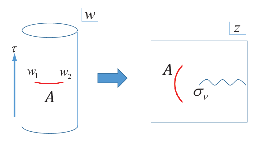
where we defined $\nu\equiv\frac{q}{2\pi}\Phi=\frac{q}{2\pi}LA_{x}$ and $\Phi\equiv\oint dx^{\prime}A_{x}=LA_{x}$. The integral $\Phi$ is the magnetic flux inside the ring and $\nu$ is the Aharonov-Bohm (AB) phase. Now we consider the Rényi entropy, $S_{A}^{(n)}=\frac{1}{1-n}\ln\mathrm{Tr}\rho_{A}^{n}$, for one interval whose length is $l$. We compute the Rényi entropy by using the replica method and the Euclidean path integral [15]. The Euclidean coordinate is $w=x+i\tau$, where $x$ is the space coordinate and has periodicity $x\sim x+L$, and $\tau$ is the Euclidean time ($-\infty<\tau<\infty$). We define the subsystem $A$ to be the interval $x_{1}\leq x\leq x_{2}$, $\tau_{1}=\tau_{2}=0$, $x_{2}-x_{1}=l$, where $w_{1}=x_{1}$ and $w_{2}=x_{2}$ are endpoints of the interval. The Rényi entropy is expressed as the expectation value of twist operators,

where $\langle\dots\rangle_{\nu}$ is the expectation value under the boundary condition (4), and $\mathcal{T}_{n}$ and $\tilde{\mathcal{T}}_{n}$ are the twist operators whose action is

here $\phi_{i}$ denotes the $i$th replica field. To compute (5), we use the conformal map $z=e^{-i\frac{2\pi}{L}w}$. From (4), the scalar field in the $z$ plane has the following boundary condition,

The boundary condition (7) can be expressed by inserting twist operators $\sigma_{\nu}$ and $\sigma_{1-\nu}$ at $z=0$ and $z=\infty$ (See Fig.2). The action of $\sigma_{\alpha}$ is

Thus, we rewrite $\textrm{Tr}[\rho_{A}^{n}]$ in (5) as

where $z_{1,2}=e^{-i\frac{2\pi}{L}w_{1,2}}$ and $h_{n}=\frac{c}{24}(n-1/n)$ is the conformal weight of $\mathcal{T}_{n}$ and $\tilde{\mathcal{T}}_{n}$, here $c$ is the central charge.

We apply (9) to a free charged scalar field. For the free scalar field, it is useful to use the following Fourier transformation,

For free fields, the Fourier transformation diagonalizes the action of $\mathcal{T}_{n}$, $\tilde{\mathcal{T}}_{n}$ and $\mathcal{\sigma}_{\alpha}$ simultaneously,

Thus, the four point function of the twist operators in (9) become

where we used the conformal map $f(z)=1-z/z_{1}$ and $x=f(z_{2})=1-e^{-i\frac{2\pi}{L}l}$ is the cross ratio of the four points ( $|x|=2|\sin\frac{\pi l}{L}|$ ). From (9) and (12), we obtain the Rényi entropy,

where we used $\left|\frac{dw_{1,2}}{dz_{1,2}}\right|=\frac{2\pi}{L}$ and omitted the irrelevant constant.

The four point function of twist operators also appear in the calculation of Rényi entropy of two disjoint intervals in free scalar field theory [29]. In the case of two disjoint intervals, the necessary four point function is $\langle\mathcal{\sigma}_{k/n}(0)\mathcal{\sigma}_{1-k/n}(x)\mathcal{\sigma}_{k/n}(1)\mathcal{\sigma}_{1-k/n}(\infty)\rangle$. In our case, we need the more general four point function $\langle\mathcal{\sigma}_{k_{1}/n}(0)\mathcal{\sigma}_{1-k_{1}/n}(x)\mathcal{\sigma}_{k_{3}/n}(1)\mathcal{\sigma}_{1-k_{3}/n}(\infty)\rangle$. In the following we will use the results of the four point function of the twist operators by Knizhnik [30]. We give derivation and different expression of $\langle\mathcal{\sigma}_{k_{1}/n}(0)\mathcal{\sigma}_{1-k_{1}/n}(x)\mathcal{\sigma}_{k_{3}/n}(1)\mathcal{\sigma}_{1-k_{3}/n}(\infty)\rangle$ by another method in the Appendix B. Note that there are a series of papers from late eighties about conformal field theories on orbifold (e.g. [31, 32, 33]) that are probably useful for more complicated cases.

The four point function of the twist operators is given by (see equations (7.22) and (7.28) in [30]),

where $\kappa$ is a constant and $\int d^{2}z=\int_{-\infty}^{\infty}d\mathrm{Re}z~\int_{-\infty}^{\infty}d\mathrm{Im}z$. Note that $\mathcal{\sigma}_{k/n}$ in [30] (and in (14)) is normalized as $\langle\mathcal{\sigma}_{k/n}(0)\mathcal{\sigma}_{1-k/n}(x)\rangle=|x|^{-2\frac{k}{n}\left(1-\frac{k}{n}\right)}$. On the other hand, $\mathcal{\sigma}_{k/n}$ in (13) is normalized as $\langle\mathcal{\sigma}_{k/n}(0)\mathcal{\sigma}_{1-k/n}(x)\rangle=\left(|x|/\epsilon\right)^{-2\frac{k}{n}\left(1-\frac{k}{n}\right)}$, here $\epsilon\equiv a/L$ and $a$ is the UV cutoff length. The latter normalization is usually used in calculation of Rényi entropy and gives the correct UV cutoff dependence of Rényi entropy. The integral $I(a,b,c,x)$ is calculated in the Appendix A. Note that the expression of $I(a,b,c,x)$ in the Appendix in [30] is not useful when $a+b=-1$ and we give a different expression which is useful when $a+b=-1$ in (26). Thus, from (13)-(17), we obtain the Rényi entropy,

where $F(\alpha,\beta,\gamma,z)$ is the Gaussian hypergeometric function,

and we used (30) in the second equality and (29) in the third equality in (18).

We study properties of the Rényi entropy (18). From (18), when $\nu\to 0$, $S_{A}^{(n)}$ diverges as

This divergence does not depend on the length of the subsystem, so it is the contribution of the homogeneous mode. This divergence is similar to the infrared divergence of the entanglement entropy in the massless limit in a free massive scalar field [34] and has the similar heuristic explanation. The correlation function is given by,

where we used $w=x+i\tau$ coordinates and $\tau=0$. From (21), the typical size of the fluctuations on the homogeneous mode grows as $(1/\nu)^{1/2}$. Correspondingly, the Rényi entropy grows as the logarithm of this volume in field space [35], and becomes $S_{A}^{(n)}\simeq 2\times\ln(1/\nu)^{1/2}=\ln(1/\nu)$. Note that we doubled the entropy because $\phi^{\prime}$ is a complex field and has the real part and the imaginary part.

We plot the $S_{A}^{(n=2)}$ as a function of $\nu$ and the length of the subsystem $l$ ( $|x|=2|\sin\frac{\pi l}{L}|$ ) in Fig.3 and Fig.4. In these figures, we have set $\kappa=1$ and $\epsilon=1$. The Rényi entropy $S_{A}^{(n=2)}$ diverges when $\nu\to 0$ and $\nu\to 1$ as shown in Fig.3. $S_{A}^{(n=2)}$ becomes a minimum value when $\nu=1/2$.

It is difficult to perform the analytical continuation of the Rényi entropy and to obtain the entanglement entropy because of the complexity of the expression (18). However, we can perform the analytical continuation in the limit $|x|\to 0$ and $\nu\to 0$. From (18), when $|x|\to 0$, we obtain

where

here $\psi(y)$ is the digamma function, $\psi(y)=\frac{d}{dy}\ln\Gamma(y)$, and we omitted the irrelevant constant $-\ln\kappa^{2}$. From (22), when $|x|\to 0$ and $\nu\to 0$, we obtain

The first term is the same as the Rényi entropy for a free massless complex scalar field and the second term is the correction from the AB phase. Thus, when $|x|\to 0$ and $\nu\to 0$, we obtain the entanglement entropy,

We studied the dependence of entanglement entropy with the AB phase in (1+1) dimensional conformal field theory on a one dimensional ring. We performed the gauge transformation (3) and the effect of AB phase is represented by the twisted boundary condition of the scalar field (4). We used the conformal map and the boundary condition was expressed by inserting twist operators $\sigma_{\nu}$ and $\sigma_{1-\nu}$ at $z=0$ and $z=\infty$ in (9). We calculated exactly the Rényi entropy in charged free scalar field theory in (18). The Rényi entropy diverges when $\nu\to 0$. This divergence comes from the homogeneous mode and is similar to the infrared divergence of the entanglement entropy in a free massive scalar field. We gave the heuristic explanation of this divergence. We performed the analytical continuation in the limit $|x|\to 0$ and $\nu\to 0$ and obtained the entanglement entropy in (25).

We considered the ground state in the presence of the AB phase (i.e. the Wilson loop). This state is a kind of excited states in CFT without the AB phase. Entanglement entropy has been studied to quantify excited states in [36, 37, 38, 39]. It is an interesting future problem to apply our method that the effect of AB phase is expressed by inserting twist operators to time dependent problems and excited states in the presence of the AB phase.

References

• [1] S. Ryu and T. Takayanagi, “Holographic derivation of entanglement entropy from AdS/CFT,” Phys. Rev. Lett. 96 (2006) 181602; “Aspects of holographic entanglement entropy,” JHEP 0608 (2006) 045.
• [2] T. Faulkner, A. Lewkowycz and J. Maldacena, “Quantum corrections to holographic entanglement entropy,” JHEP 1311, 074 (2013) [arXiv:1307.2892].
• [3] B. Swingle, ”Entanglement Renormalization and Holography,” Phys. Rev. D 86, 065007 (2012), arXiv:0905.1317 [cond-mat.str-el].
• [4] M. Nozaki, S. Ryu and T. Takayanagi, ”Holographic Geometry of Entanglement Renormalization in Quantum Field Theories,” JHEP 1210 (2012) 193, arXiv:1208.3469 [hep-th].
• [5] M. Miyaji and T. Takayanagi, ”Surface/State Correspondence as a Generalized Holography,” PTEP 2015 (2015) no.7, 073B03, arXiv:1503.03542[hep-th].
• [6] M. Rangamani, T. Takayanagi, ”Holographic Entanglement Entropy, ” arXiv:1609.01287 [hep-th].
• [7] N. Shiba, T. Takayanagi, “Volume Law for the Entanglement Entropy in Non-local QFTs,” JHEP 1402 (2014) 033, arXiv:1311.1643 [hep-th].
• [8] A. Mollabashi, N. Shiba, T. Takayanagi, “Entanglement between Two Interacting CFTs and Generalized Holographic Entanglement Entropy,” JHEP 1404 (2014) 185, arXiv:1403.1393 [hep-th].
• [9] M. Miyaji, T. Numasawa, N. Shiba, H. Takayanagi, K. Watanabe, “Continuous Multiscale Entanglement Renormalization Ansatz as Holographic Surface-State Correspondence,” Phys.Rev.Lett. 115 (2015) no.17, 171602, arXiv:1506.01353 [hep-th].
• [10] M. Miyaji, T. Numasawa, N. Shiba, H. Takayanagi, K. Watanabe, “Distance between Quantum States and Gauge-Gravity Duality,” Phys.Rev.Lett. 115 (2015) no.26, 261602, arXiv:1507.07555 [hep-th].
• [11] T. Miyagawa, N. Shiba, H. Takayanagi, “Double-Trace Deformations and Entanglement Entropy in AdS,” Fortsch.Phys. 64 (2016) 92-105, arXiv:1511.07194 [hep-th].
• [12] T. Numasawa, N. Shiba, H. Takayanagi, K. Watanabe, “EPR Pairs, Local Projections and Quantum Teleportation in Holography,” JHEP 1608 (2016) 077, arXiv:1604.01772 [hep-th].
• [13] M. Levin and X.-G. Wen, “Detecting Topological Order in a Ground State Wave Function,” Phys. Rev. Lett. 96, 110405 (2006), arXiv:cond-mat/0510613.
• [14] A. Kitaev and J. Preskill, “Topological entanglement entropy,” Phys. Rev. Lett. 96, 110404 (2006), arXiv:hep-th/0510092
• [15] P. Calabrese and J. Cardy, “Entanglement entropy and quantum field theory,” J. Stat. Mech. 0406, P002 (2004), arXiv:hep-th/0405152
• [16] S. Ghosh, R. M. Soni, S. P. Trivedi, ”On The Entanglement Entropy For Gauge Theories, ” JHEP 1509 (2015) 069 , arXiv:1501.02593 [hep-th].
• [17] S. Aoki, T. Iritani, M. Nozaki, T. Numasawa, N. Shiba, H. Tasaki, “ On the definition of entanglement entropy in lattice gauge theories,” JHEP 1506 (2015) 187, arXiv:1502.04267 [hep-th].
• [18] L. Bombelli, R. K. Koul, J. Lee and R. D. Sorkin, “A Quantum Source of Entropy for Black Holes,” Phys. Rev. D 34 (1986) 373.
• [19] M. Srednicki, “Entropy and area,” Phys. Rev. Lett. 71 (1993) 666 [hep-th/9303048].
• [20] L. Susskind and J. Uglum, ”Black hole entropy in canonical quantum gravity and superstring theory,” Phys. Rev. D 50, 2700 (1994), arXiv:hep-th/9401070.
• [21] D. N. Kabat, ”Black hole entropy and entropy of entanglement,” Nucl. Phys. B 453, 281 (1995), arXiv:hep-th/9503016.
• [22] N. Shiba, “Entanglement Entropy of Two Black Holes and Entanglement Entropic Force,” Phys.Rev. D83 (2011) 065002, arXiv:1011.3760 [hep-th].
• [23] N. Shiba, “Entanglement Entropy of Two Spheres,” JHEP 1207 (2012) 100, arXiv:1201.4865 [hep-th].
• [24] R. E. Arias, D. D. Blanco, H. Casini, ”Entanglement entropy as a witness of the Aharonov-Bohm effect in QFT,” J.Phys. A48 (2015) no.14, 145401, arXiv:1409.3269 [hep-th]
• [25] L. Chojnacki, C. Q. Cook, D. Dalidovich, L. E. H. Sierens, É. Lantagne-Hurtubise, R. G. Melko, T. J. Vlaar, ”Shape dependence of two-cylinder Renyi entropies for free bosons on a lattice,” Phys. Rev. B 94, 165136 (2016), arXiv:1607.05311 [cond-mat.str-el]
• [26] M. A. Metlitski, C. A. Fuertes, S. Sachdev ”Entanglement Entropy in the O(N) model,” Phys. Rev. B 80, 115122 (2009), arXiv:0904.4477 [cond-mat.stat-mech]
• [27] S. Whitsitt, W. Witczak-Krempa, S. Sachdev ”Entanglement entropy of the large N Wilson-Fisher conformal field theory,” Phys. Rev. B 95, 045148 (2017) arXiv:1610.06568 [cond-mat.str-el]
• [28] X. Chen, W. Witczak-Krempa, T. Faulkner, E. Fradkin ”Two-cylinder entanglement entropy under a twist,” J.Stat.Mech. 1704 (2017) no.4, 043104 arXiv:1611.01847 [cond-mat.str-el]
• [29] P. Calabrese, J. Cardy, E. Tonni, ”Entanglement entropy of two disjoint intervals in conformal field theory, ” J.Stat.Mech. 0911 (2009) P11001, arXiv:0905.2069 [hep-th].
• [30] V. G. Knizhnik, ”Analytic fields on Riemann surfaces. II,” Communn. Math. Phys. 112, 567 (1987).
• [31] L. J. Dixon, D. Friedan, E. J. Martinec and S. H. Shenker, ”The Conformal Field Theory Of Orbifolds,” Nucl. Phys. B 282 (1987) 13.
• [32] M. Bershadsky and A. Radul, ”Conformal field theories with additional ZNZ_{N} symmetry,” Int. J. Mod. Phys. A 2, 165 (1987).
• [33] J. J. Atick, L. J. Dixon, P. A. Griffin and D. Nemeschansky, ”Multiloops twist field correlation functions for Z(N) orbifolds,” Nucl. Phys. B 298 (1988) 1.
• [34] H. Casini and M. Huerta, “Entanglement entropy in free quantum field theory,” J.Phys. A42 (2009) 504007, arXiv:0905.2562 [hep-th].
• [35] W. G. Unruh, ”Comment on ‘Proof of the quantum bound on specific entropy for free fields’ ,” Phys. Rev. D 42, 3596 (1990).
• [36] M. Nozaki, T. Numasawa and T. Takayanagi, ”Quantum Entanglement of Local Operators in Conformal Field Theories,” Phys. Rev. Lett. 112, 111602 (2014) [arXiv:1401.0539 [hep-th]].
• [37] S. He, T. Numasawa, T. Takayanagi and K. Watanabe, ”Quantum Dimension as Entanglement Entropy in 2D CFTs,” Phys.Rev. D90 (2014) no.4, 041701, arXiv:1403.0702 [hep-th].
• [38] F. C. Alcaraz, M. I. Berganza, G. Sierra, Phys. Rev. Lett. 106 (2011) 201601 [arXiv:1101.2881 [cond-mat]].
• [39] N. Shiba, “Entanglement Entropy of Disjoint Regions in Excited States : An Operator Method,” JHEP 1412 (2014) 152, arXiv:1408.0637 [hep-th].
• [40] H. Kawai, D.C. Lewellen, S.-H. H. Tye, ”A Relation Between Tree Amplitudes of Closed and Open Strings,” Nucl.Phys. B269 (1986) 1-23.