Equivariant Versions of Odd Number Theorem

Suppose that system (11) has a periodic solution $x^{*}$ with period $T$. Assume that this system respects some group of symmetries, and for one particular $g$ relation (4) holds. We denote by $\Phi(t)$ the fundamental matrix of the linearization

$$\dot{y}=B(t)y,\qquad B(t):=Df_{x}(x^{*}(t)),$$

(6)

of system (11) near $x^{*}(t)$, where $Df_{x}$ denotes the Jacobi matrix of $f$. Condition (4) implies that

$$A_{g}^{-1}\Phi(T_{g})\psi(0)=\psi(0),\qquad\psi(t):=\dot{x}^{*}(t),$$

(7)

i.e. the matrix $A_{g}^{-1}\Phi(T_{g})$ has an eigenvalue $1$. We assume that

$(H_{1})$ $1$ is a simple eigenvalue for the matrix $A_{g}^{-1}\Phi(T_{g})$.

Following [14], we introduce a modified Pyragas control as in (5), where we assume that

$$KA_{g}=A_{g}K.$$

(8)

This commutativity property can be a natural restriction on feasible controls. For example, it is typical of laser systems. On the other hand, gain matrices, which are simple enough to allow for efficient analysis of stability of the controlled equation (5), also usually satisfy condition (8) (cf. [11, 16]).

Let $D^{\prime}$ denote the transpose of a matrix $D$. Using $(H_{1})$, denote by $\psi^{\dagger}$ the normalized adjoint eigenvector with the eigenvalue $1$ for the matrix $[A_{g}^{-1}\Phi(T_{g})]^{\prime}$:

$$[A_{g}^{-1}\Phi(T_{g})]^{\prime}\psi_{0}^{\dagger}=\psi_{0}^{\dagger};\qquad\psi_{0}^{\dagger}\cdot\psi(0)=1,$$

where dot denotes the standard scalar product in $\mathbb{R}^{n}$. Furthermore, denote by $\psi^{\dagger}(t)$ the solution of the initial value problem

$$\dot{y}=-B^{\prime}(t)y;\qquad y(0)=\psi_{0}^{\dagger}.$$

Since the fundamental matrix of system $\dot{y}=-B^{\prime}(t)y$ is $(\Phi^{-1}(t))^{\prime}$,

$$\psi^{\dagger}(t)=(\Phi^{-1}(t))^{\prime}\psi^{\dagger}_{0}.$$

(9)

Note that relation (4) implies

$$A_{g}\psi(t)=\psi(t+T_{g});\qquad A_{g}^{\prime}\psi^{\dagger}(t)=\psi^{\dagger}(t-T_{g}).$$

Finally denote by $N$ the number of real eigenvalues $\mu$ of the matrix $A_{g}^{-1}\Phi(T_{g})$, which satisfy $\mu>1$.

Hence, the inequality opposite to (10) is a necessary condition for stabilization of the periodic solution $x^{*}$. This necessary condition restricts the choice of the gain matrix $K$.

As an illustrative example of Theorem 2.1 we consider the system of two identical diffusely coupled Landau oscillators described in complex form by

	$\displaystyle\dot{z}_{1}$	$\displaystyle=(\alpha+i+\gamma|z_{1}|^{2})z_{1}+a(z_{2}-z_{1}),$		(11)
	$\displaystyle\dot{z}_{2}$	$\displaystyle=(\alpha+i+\gamma|z_{2}|^{2})z_{2}+a(z_{1}-z_{2})$

with $z_{1},z_{2}\in\mathbb{C}$. Here $\alpha$ and $a>0$ are real parameters while $\gamma$ is a complex parameter with ${\rm Re}\,\gamma>0$. When $\alpha$ is treated as a bifurcation parameter, this system undergoes two sub-critical Hopf bifurcations, the first at $\alpha=0$ giving rise to a fully synchronized branch of solutions and the second at $\alpha=2a$ giving rise to an anti-phase branch. The anti-phase branch is defined for $\alpha<2a$ and is given explicitly by the formula

$$z_{1}^{*}(t)=-z_{2}^{*}(t)=r(\alpha)e^{i\omega(\alpha)t},$$

(12)

where $r=r(\alpha):=\sqrt{({2a-\alpha})/{{\rm Re}\,\gamma}}$ and $\omega=\omega(\alpha):=1+r^{2}(\alpha){\rm Im}\,\gamma$. In [4] this branch was stabilized by introducing equivariant Pyragas control to system (11) in the following way:

	$\displaystyle\dot{z}_{1}$	$\displaystyle=(\alpha+i+\gamma|z_{1}|^{2})z_{1}+a(z_{2}-z_{1})+b(z_{2}(t-{\pi}/{\omega})-z_{1})),$		(13)
	$\displaystyle\dot{z}_{2}$	$\displaystyle=(\alpha+i+\gamma|z_{2}|^{2})z_{2}+a(z_{1}-z_{2})+b(z_{1}(t-{\pi}/{\omega})-z_{2}))$

with a complex gain parameter $b$. To study stability of the anti-phase branch close to the bifurcation point in system (13), linear stability analysis of the origin combined with explicit knowledge of the branch made it possible to find sufficient conditions under which for some interval of $\alpha$ sufficiently close to $2a$ the branch is stable.

Due to the simple nature of the Landau oscillator, explicit computation of the fundamental matrix of the linearization of system (11) near the solution (12) allows us to compute expression (10). This gives us the following necessary condition for stabilization of any of the anti-phase cycles (12):

$$1+\pi\,\frac{{\rm Re}\,\gamma\,{\rm Re}\,b+{\rm Im}\,\gamma\,{\rm Im}\,b}{\omega{\rm Re}\,\gamma}<0.$$

(14)

At the point $\alpha=2a$, $\omega=1$, this coincides with formula (6.10) from [4] which, together with other conditions, defines the stability domain for small periodic orbits. In particular, for a fixed gain parameter $b$, condition (14) provides an upper bound for the interval of $\alpha$ where the anti-phase cycle is stable.

Linearizing system (5) near $x^{*}$ gives

$$\dot{y}(t)=B(t)y(t)+K(A_{g}y(t-T_{g})-y(t)).$$

(15)

To prove that $x^{*}$ is an unstable periodic solution of (5) we will show that system (15) has a solution

$$y_{\mu}^{*}(t)=\mu^{t/T_{g}}p(t),\qquad A_{g}p(t-T_{g})=p(t)$$

(16)

with $\mu>1$, where the relation $A_{g}p(t-T_{g})=p(t)$ ensures that $p$ is periodic. It is easy to see that if the ordinary differential system

$$\dot{y}=\left(B(t)+(\mu^{-1}-1)K\right)y$$

(17)

has a solution $y_{\mu}$ of type (16), then $y_{\mu}$ is also a solution of (15). Denote by $\Psi_{\mu}(t)$ the fundamental matrix of (17).

The proof of this lemma is presented in the next subsection. In order to use Lemma 2.2, we consider the characteristic polynomial

$$F(\mu):=\det\left(\mu\,\mathbb{I}\text{d}-A_{g}^{-1}\Psi_{\mu}(T_{g})\right)$$

of the matrix $A_{g}^{-1}\Psi_{\mu}(T_{g})$. Observe that equation (17) with $\mu=1$ coincides with (6), hence $\Psi_{1}=\Phi$ and therefore condition ($H_{1}$) implies $F(1)=0$. We are going to show that relation (10) implies

$$F(1+\varepsilon)<0,\qquad 0<\varepsilon\ll 1.$$

(18)

Since $F(\mu)\to+\infty$ as ${\mu\to+\infty}$, relation (18) implies that $F$ has a root $\mu>1$ and therefore the conclusion of Theorem 2.1 follows from (18) by Lemma 2.2.

Setting $\mu=1+\varepsilon$ and $t=T_{g}$ in the identity

$$\Psi_{\mu}(t)=\Phi(t)\left(\mathbb{I}\text{d}+(\mu^{-1}-1)\int_{0}^{t}\Phi^{-1}(s)K\Psi_{\mu}(s)\,ds\right)$$

and using the fact that $\Psi_{1+\varepsilon}(T_{g})=\Phi(T_{g})+O(\varepsilon)$, we obtain the expansion

$$\Psi_{1+\varepsilon}(T_{g})=\Phi(T_{g})\left(\mathbb{I}\text{d}-\varepsilon Q\right)+O(\varepsilon^{2}),\qquad Q:=\int_{0}^{T_{g}}\Phi^{-1}(t)K\Phi(t)\,dt.$$

Therefore,

$$\begin{array}[]{rcl}F(1+\varepsilon)=\det\left(\text{Id}-A_{g}^{-1}\Phi(T_{g})+\varepsilon\left(\mathbb{I}\text{d}+A_{g}^{-1}\Phi(T_{g})Q\right)\right)+O(\varepsilon^{2}).\end{array}$$

(19)

Let us denote by $L$ the transition matrix to a basis in which the matrix $A_{g}^{-1}\Phi(T_{g})$ assumes the Jordan form and agree that $\psi(0)$ is the first vector of this basis (cf. (7)), i.e.

$$Le_{1}=\psi(0),\qquad e_{1}:=(1,0,\ldots,0)^{\prime}\in\mathbb{R}^{n}.$$

(20)

In this basis, the matrix $\text{Id}-L^{-1}A_{g}^{-1}\Phi(T_{g})L$ has the Jordan structure with the diagonal entries $0,1-\mu_{2},1-\mu_{3},\ldots,1-\mu_{n}$, where $\mu_{k}$ are the eigenvalues of $A_{g}^{-1}\Phi(T_{g})$ different from the simple eigenvalue $1$. With this notation, formula (19) implies

$$F(1+\varepsilon)=\varepsilon M_{11}\prod^{n}_{k=2}(1-\mu_{k})+O(\varepsilon^{2}),$$

(21)

where

$$M:=\mathbb{I}\text{d}+L^{-1}A_{g}^{-1}\Phi(T_{g})QL;\qquad M_{11}=e_{1}\cdot Me_{1}.$$

(22)

Formula (3.2) implies that $(L^{-1})^{\prime}e_{1}=\psi_{0}^{\dagger}$, hence

$$e_{1}\cdot L^{-1}QLe_{1}=\int_{0}^{T_{g}}\psi_{0}^{\dagger}\cdot\Phi^{-1}(t)K\Phi(t)\psi(0)\,dt.$$

Combining this with (3.2) and $\psi(t)=\Phi(t)\psi(0)$, we obtain

$$e_{1}\cdot L^{-1}QLe_{1}=\int_{0}^{T_{g}}\psi^{\dagger}(t)K\psi(t)\,dt.$$

Since the first row of the matrix $L^{-1}A_{g}^{-1}\Phi(T_{g})L$ is $(e_{1})^{\prime}=(1,0,\ldots,0)$, we see from (31) that

$$M_{11}=1+e_{1}\cdot L^{-1}QLe_{1}=1+\int_{0}^{T_{g}}\psi^{\dagger}(t)K\psi(t)\,dt.$$

Hence (30) implies

$${\rm sgn}\,F(1+\varepsilon)=(-1)^{N}\left(1+\int_{0}^{T_{g}}\psi^{\dagger}(t)K\psi(t)\,dt\right),$$

where $N$ is the number of eigenvalues $\mu_{k}$ satisfying $\mu_{k}>1$. Thus, formula (10) indeed implies (18).

Let us denote

$$C(t):=B(t)+(\mu^{-1}-1)K.$$

The main ingredient for the proof is the identity

$$C(t+T_{g})=A_{g}C(t)A_{g}^{-1},$$

which is a simple consequence of the facts that $Df(A_{g}x)=A_{g}Df(x)A_{g}^{-1}$, $x^{*}(t+T_{g})=A_{g}x^{*}(t)$, and $A_{g}K=KA_{g}$.

To complete the proof denote by $\nu$ the eigenvector of $A_{g}^{-1}\Psi_{\mu}$ with the eigenvalue $\mu$ and consider the solution $y_{0}(t)$ of (17) with $y_{0}(0)=\nu$. It is clear that $y_{0}(t+T_{g})$ satisfies the initial value problem

$$\begin{cases}\dot{y}_{1}=C(t+T_{g})y_{1}=A_{g}C(t)A_{g}^{-1}y_{1},\\ y_{1}(0)=\Psi(T_{g})\nu.\end{cases}$$

(23)

By the change of variables $y_{2}=A_{g}^{-1}y_{1}$, we can see that the solution of (23) is given by

$$y_{0}(t+T_{g})=y_{1}(t)=A_{g}\Psi(t)A_{g}^{-1}\Psi(T_{g})\nu.$$

However by assumption $A_{g}^{-1}\Psi(T_{g})\nu=\mu\nu$, hence

$$y_{0}(t+T_{g})=\mu A_{g}\Psi(t)\nu=\mu A_{g}y_{0}(t),$$

which proves the lemma.

Suppose that equation (11) is $S^{1}$-equivariant:

$$f(e^{\theta J}x)=e^{\theta J}f(x)$$

(24)

for all $\theta\in\mathbb{R}$, $x\in\mathbb{R}^{N}$, where the skew-symmetric non-zero matrix $J$ satisfies $e^{2\pi J}=\mathbb{I}{\rm d}$. We assume that (11) has a periodic solution $x^{*}(t)$ of a period $T$, which is not a relative equilibrium. Hence, equation (11) has an orbit of $T$-periodic non-stationary solutions $e^{\theta J}x^{*}(t+\tau)$ with arbitrary $\theta,\tau$. Therefore, the linearization (6) has two linearly independent zero modes (periodic solutions):

$$\psi_{1}(t)=\dot{x}^{*}(t),\qquad\psi_{2}(t)=Jx^{*}(t)$$

(25)

with the Floquet multiplier $1$. We additionally assume that

$(H_{2})$ The eigenvalue $1$ of the monodromy matrix $\Phi(T)$ of system (6) has multiplicity exactly $2$.

Then, there are two adjoint eigenfunctions (periodic solutions of equation $\dot{y}=-B(t)y$) that can be normalized as follows:

$$\psi_{1}^{\dagger}(t)\cdot\psi_{1}(t)=\psi_{2}^{\dagger}(t)\cdot\psi_{2}(t)\equiv 1,\qquad\psi_{1}^{\dagger}(t)\cdot\psi_{2}(t)=\psi_{2}^{\dagger}(t)\cdot\psi_{1}(t)\equiv 0.$$

(26)

Up to the asymptotic expansion (19) the proof of Theorem 3.1 is a modification of the proof of Theorem 2.1 where $A_{g}$ is replaced by the identity matrix $\mathbb{I}\text{d}$ and $T_{g}$ is replaced by $T$. In this case, the counterpart of relation (19) is given by

$$F(1+\varepsilon)=\det\left(\mathbb{I}\text{d}-\Phi(T)+\varepsilon\left(\mathbb{I}\text{d}+\Phi(T)\int_{0}^{T}\Phi^{-1}(t)K\Phi(t)\,dt\right)+O(\varepsilon^{2})\right).$$

(29)

We again denote by $L$ the transition matrix to a basis in which the matrix $\Phi(T)$ assumes the Jordan form and agree that $\psi_{1}(0)$ and $\psi_{2}(0)$ are the first and second vector of this basis (cf. (25)), i.e.

	$\displaystyle Le_{1}=$	$\displaystyle\psi_{1}(0),\qquad e_{1}:=(1,0,\ldots,0)^{\prime}\in\mathbb{R}^{n},$
	$\displaystyle Le_{2}=$	$\displaystyle\psi_{2}(0),\qquad e_{2}:=(0,1,\ldots,0)^{\prime}\in\mathbb{R}^{n}.$

In this basis, the matrix $\text{Id}-L^{-1}\Phi(T)L$ has the Jordan structure with the diagonal entries $0,0,1-\mu_{3},\ldots,1-\mu_{n}$, where $\mu_{k}$ are the eigenvalues of $\Phi(T)$, which are different from $1$. With this notation, formula (29) implies

$$F(1+\varepsilon)=\varepsilon^{2}(M_{11}M_{22}-M_{12}M_{21})\prod^{n}_{k=3}(1-\mu_{k})+O(\varepsilon^{3}),$$

(30)

where

$$M:=\mathbb{I}\text{d}+L^{-1}\Phi(T)\left(\int_{0}^{T}\Phi^{-1}(t)K\Phi(t)\,dt\right)L;\qquad M_{ij}=e_{i}\cdot Me_{j}.$$

(31)

The same argument as in the proof of Theorem 2.1 shows that

$${\rm sgn}\,F(1+\varepsilon)=(-1)^{N}\bigl((1+c_{11})(1+c_{22})-c_{12}c_{21}\bigr),$$

where $c_{ij}$ is defined by (28). Combining this with the case of Lemma 2.2 where $A_{g}=\text{Id}$ and $T_{g}=T$, and the fact that $F(\mu)\to+\infty$ as $\mu\to+\infty$ completes the proof.

In order to illustrate Theorem 3.1, we consider a model of two coupled lasers, see for example [23]. In dimensionless form, the rate equations describing this system can be written as

	$\displaystyle\dot{E}_{1}$	$\displaystyle=$	$\displaystyle i\delta E_{1}+(1+i\alpha)N_{1}E_{1}+\eta e^{-i\varphi}E_{2},$		(32)
	$\displaystyle\dot{N}_{1}$	$\displaystyle=$	$\displaystyle\varepsilon\left[J-N_{1}-(1+2N_{1})|E_{1}|^{2}\right],$		(33)
	$\displaystyle\dot{E}_{2}$	$\displaystyle=$	$\displaystyle(1+i\alpha)N_{2}E_{2}+\eta e^{-i\varphi}E_{1},$		(34)
	$\displaystyle\dot{N}_{2}$	$\displaystyle=$	$\displaystyle\varepsilon\left[J-N_{2}-(1+2N_{2})|E_{2}|^{2}\right],$		(35)

where the complex-valued variables $E_{1}$, $E_{2}$ are optical fields and the real-valued variables $N_{1}$, $N_{2}$ are carrier densities in two laser cavities, respectively. This system is symmetric under the action of the group $S^{1}$ of transformations $\left(E_{1},N_{1},E_{2},N_{2}\right)\to\left(e^{i\theta}E_{1},N_{1},e^{i\theta}E_{2},N_{2}\right)$. Hence, the system admits relative equilibria of the form

$$\left(E_{1},N_{1},E_{2},N_{2}\right)=\left(a_{1}e^{i\omega t},n_{1},a_{2}e^{i\omega t},n_{2}\right)$$

(36)

with $\omega,n_{1},n_{2}\in\mathbb{R}$ and $a_{1},a_{2}\in\mathbb{C}$. The problem of stabilization of unstable relative equilibria for this system was considered in [5]. System (32)–(35) can also have relative periodic orbits, i.e. solutions of the form

$$(e^{i\omega t}E_{1}^{*}(t),N_{1}^{*}(t),e^{i\omega t}E_{2}^{*}(t),N_{2}^{*}(t)),$$

(37)

where $E_{1}^{*}(t),N_{1}^{*}(t),E_{2}^{*}(t),N_{2}^{*}(t)$ are $T$-periodic. In the present section we choose a relative periodic solution as a target state for stabilization.

In order to stabilize the solution (37), we add the modified Pyragas control term

$$E_{b}(t):=b_{0}\,e^{i\beta}\left(e^{-i\omega T}E_{1}(t-T)-E_{1}(t)\right)$$

(38)

to the right hand side of equation (32). Here the parameters $b_{0}>0$ and $\beta\in\mathbb{R}$ measure the amplitude and phase of the control, respectively; and $T$, $\omega$ are the parameters of the target relative periodic solution (37). Introducing the rotating coordinates $(\tilde{E}_{1},\tilde{N}_{1},\tilde{E}_{2},\tilde{N}_{2})=(e^{-i\omega t}E_{1},N_{1},e^{-i\omega t}E_{2},N_{2})$ transforms equations (32)–(35) to an autonomous system that has an orbit of non-stationary $T$-periodic solutions $(e^{i\theta}\tilde{E}_{1},\tilde{N}_{1},e^{i\theta}\tilde{E}_{2},\tilde{N}_{2})=(E_{1}^{*}(t+\tau),N_{1}^{*}(t+\tau),E_{2}^{*}(t+\tau),N_{2}^{*}(t+\tau))$ with arbitrary $\theta,\tau$. This change of variables transforms the control term (38) to the standard Pyragas form

$$\tilde{E}_{b}(t)=b_{0}e^{i\beta}(\tilde{E}_{1}(t-\tau)-\tilde{E}_{1}(t)).$$

(39)

Hence, we can use Theorem 3.1 to establish the values of $b_{0}$ and $\beta$ for which the control cannot stabilize the solution (37).

Following the analysis presented in [5], we use the phase $\varphi$ of coupling between the lasers as the bifurcation parameter. Varying $\varphi$ one observes Hopf bifurcations on the branches of relative equilibria. These bifurcations give rise to branches of relative periodic solutions (which are just periodic solutions in the rotating coordinates). Figure 1 features the bifurcation diagram for system (32)–(35) with the same parameter set as in [5]. We are interested in the unstable part of the branch of relative periodic solutions born via a subcritical Hopf bifurcation.

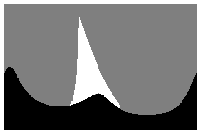
Figure 2 shows three regions in the parameter space $(\beta,b_{0})$. The black region corresponds to the values of $b_{0}$ and $\beta$ for which condition (27) is satisfied, hence the target state is not stabilizable by control (38). The white and gray regions correspond to stable and unstable target state in the controlled system, respectively. Figure 3 shows the change of the spectrum of the target state after applying Pyragas control (38).

It would be interesting to consider symmetric coupling of laser models of other types such as for example in [21, 22, 10, 20, 9, 7].

The authors acknowledge the support of NSF through grant DMS-$1413223$.

References

- [1] G Brown, CM Postlethwaite, and M Silber. Time-delayed feedback control of unstable periodic orbits near a subcritical hopf bifurcation. Physica D: Nonlinear Phenomena, 240(9):859–871, 2011.
- [2] K Engelborghs, T Luzyanina, and D Roose. Numerical bifurcation analysis of delay differential equations using dde-biftool. ACM Trans. Math. Softw., 28(1):1–21, 2002.
- [3] K Engelborghs, T Luzyanina, and G Samaey. Dde-biftool v. 2.00: A matlab package for bifurcation analysis of delay differential equations. department of computer science. Technical report, KU Leuven, Technical Report TW-330, Leuven, Belgium, 2001.
- [4] B Fiedler, V Flunkert, P Hövel, and E Schöll. Delay stabilization of periodic orbits in coupled oscillator systems. Philosophical Transactions of the Royal Society of London A: Mathematical, Physical and Engineering Sciences, 368:319–341, 2010.
- [5] B Fiedler, S Yanchuk, V Flunkert, P Hövel, H-J Wünsche, and E Schöll. Delay stabilization of rotating waves near fold bifurcation and application to all-optical control of a semiconductor laser. Physical Review E, 77:066207, 2008.
- [6] EW Hooton and A Amann. Analytical limitation for time-delayed feedback control in autonomous systems. Physical Review Letters, 109(15):154101, 2012.
- [7] L Jaurigue, A Pimenov, D Rachinskii, E Schöll, K Lüdge, and AG Vladimirov. Timing jitter of passively-mode-locked semiconductor lasers subject to optical feedback: A semi-analytic approach. Physical Review A, 92(5):053807, 2005.
- [8] H Nakajima. On analytical properties of delayed feedback control of chaos. Physics Letters A, 232(3):207–210, 1997.
- [9] M Nizette, D Rachinskii, A Vladimirov, and M Wolfrum. Pulse interaction via gain and loss dynamics in passive mode locking. Physica D: Nonlinear Phenomena, 218(1):95–104, 2006.
- [10] A Pimenov, EA Viktorov, SP Hegarty, T Habruseva, G Huyet, D Rachinskii, and Vladimirov AG. Bistability and hysteresis in an optically injected two-section semiconductor laser. Physical Review E, 89(5):052903, 2014.
- [11] CM Postlethwaite, G Brown, and M Silber. Feedback control of unstable periodic orbits in equivariant Hopf bifurcation problems. Phil. Trans. R. Soc. A, 371(1999):20120467, 2013.
- [12] K Pyragas. Continuous control of chaos by self-controlling feedback. Physics Letters A, 170:421–428, 1992.
- [13] S Schikora, P Hövel, H-J Wünsche, E Schöll, and F Henneberger. All-optical noninvasive control of unstable steady states in a semiconductor laser. Physical Review Letters, 97(21):213902, 2006.
- [14] I Schneider. Delayed feedback control of three diffusively coupled Stuart–Landau oscillators: a case study in equivariant Hopf bifurcation. Philosophical Transactions of the Royal Society of London A: Mathematical, Physical and Engineering Sciences, 371:20120472, 2013.
- [15] I Schneider. Equivariant pyragas control. Master’s thesis, Freie Universität Berlin, 2014.
- [16] I Schneider and M Bosewitz. Eliminating restrictions of time-delayed feedback control using equivariance. Discrete and Continuous Dynamical Systems Series A, 36:451–467, 2016.
- [17] I Schneider and B Fiedler. Symmetry-breaking control of rotating waves. In Control of Self-Organizing Nonlinear Systems, pages 105–126. Springer, 2016.
- [18] J Sieber, A Gonzalez-Buelga, SA Neild, DJ Wagg, and B Krauskopf. Experimental continuation of periodic orbits through a fold. Physical Review Letters, 100(24):244101, 2008.
- [19] M Tlidi, AG Vladimirov, D Pieroux, and D Turaev. Spontaneous motion of cavity solitons induced by a delayed feedback. Physical Review Letters, 103(10):103904, 2009.
- [20] AG Vladimirov, D Rachinskii, and M Wolfrum. Modeling of passively modelocked semiconductor lasers, chapter viii. In Kathy Lüdge, editor, Nonlinear Laser Dynamics: From Quantum Dots to Cryptography 5, pages 189–222. Wiley-VCH, 2011.
- [21] AG Vladimirov and D Turaev. Model for passive mode locking in semiconductor lasers. Physical Review A, 72:033808, 2005.
- [22] AG Vladimirov, M Wolfrum, G Fiol, D Arsenijevic, D Bimberg, E Viktorov, P Mandel, and D Rachinskii. Locking characteristics of a 40-ghz hybrid mode-locked monolithic quantum dot laser. SPIE Photonics Europe, 7720:77200Y–77200Y–8, 2010.
- [23] S Yanchuk, K R Schneider, and L Recke. Dynamics of two mutually coupled semiconductor lasers: Instantaneous coupling limit. Physical Review E, 69:056221, 2004.