On the solutions of a second-order difference equations in terms of generalized Padovan sequences

Yacine Halim Affiliation: Department of Mathematics and computer sceinceMila University Center, Mila, AlgeriaEmail: halyacine@yahoo.fr Julius Fergy T. Rabago Affiliation: Department of Mathematics and computer sciencesCollege of Science, University of the Philippines,Gov. Pack Road, Baguio City 2600, Benguet, Philippines.Email: jfrabago@gmail.com

Abstract

This paper deals with the solution, stability character and asymptotic behavior of the rational difference equation

x_{n+1}=\frac{\alpha x_{n-1}+\beta}{\gamma x_{n}x_{n-1}},\qquad n\in\mathbb{N}_{0},

where $\mathbb{N}_{0}=\mathbb{N}\cup\left\{0\right\}$ , $\alpha,\beta,\gamma\in\mathbb{R}^{+}$ , and the initial conditions $x_{-1}$ and $x_{0}$ are non zero real numbers such that their solutions are associated to generalized Padovan numbers. Also, we investigate the two-dimensional case of the this equation given by

x_{n+1}=\frac{\alpha x_{n-1}+\beta}{\gamma y_{n}x_{n-1}},\qquad y_{n+1}=\frac{\alpha y_{n-1}+\beta}{\gamma x_{n}y_{n-1}},\qquad n\in\mathbb{N}_{0},

and this generalizes the results presented in [34].
Keywords: Difference equations, general solution, stability, generalized Padovan numbers.
Mathematics Subject Classification: 39A10, 40A05.

1 Introduction and preliminaries

The term difference equation refers to a specific type of recurrence relation – a mathematical relationship expressing $x_{n}$ as some combination of $x_{i}$ with $i<n$ . These equations usually appear as discrete mathematical models of many biological and environmental phenomena such as population growth and predator-prey interactions (see, e.g., [8] and [18]), and so these equations are studied because of their rich and complex dynamics. Recently, the problem of finding closed-form solutions of rational difference equations and systems of rational of difference equations have gained considerable interest from many mathematicians. In fact, countless papers have been published previously focusing on the aforementioned topic, see for example [5, 6, 7, 16, 20] and [21]. Interestingly, some of the solution forms of these equations are even expressible in terms of well-known integer sequences such as the Fibonacci numbers, Horadam numbers and Padovan numbers (see, e.g., [9, 11, 12, 14, 22, 24, 25, 26, 27, 29, 34]).

It is well-known that linear recurrences with constant coefficients, such as the recurrence relation $F_{n+1}=F_{n}+F_{n-1}$ defining the Fibonacci numbers, can be solved through various techniques (see, e.g., [17]). Finding the closed-form solutions of nonlinear types of difference equations, however, are far more interesting and challenging compared to those of linear types. In fact, as far as we know, there has no known general method to deal with different classes of difference equations solvable in closed-forms. Nevertheless, numerous studies have recently dealt with finding appropriate techniques in solving closed-form solutions of some systems of difference equations (see, e.g., [2, 5, 6, 7, 15, 23]).

Motivated by these aforementioned works, we investigate the rational difference equation

x_{n+1}=\frac{\alpha x_{n-1}+\beta}{\gamma x_{n}x_{n-1}},\quad n\in\mathbb{N}_{0},.

(1)

Particularly, we seek to find its closed-form solution and examine the global stability of its positive solutions. We establish the solution form of equation (1) using appropriate transformation reducing the equation into a linear type difference equation. Also, we examine the solution form of the two-dimensional analogue of equation (1) given in the following more general form

x_{n+1}=\frac{\alpha x_{n-1}+\beta}{\gamma y_{n}x_{n-1}},\qquad y_{n+1}=\frac{\alpha y_{n-1}+\beta}{\gamma x_{n}y_{n-1}},\qquad n\in\mathbb{N}_{0}.

(2)

The case $\alpha=\beta=\gamma=1$ has been studied by Tollu, Yazlik and Taskara in [34]. The authors in [34] established the solution form of system (2) (in the case $\alpha=\beta=\gamma=1$ ) through induction principle.

The paper is organized as follows. In the next section (Section 2), we review some definitions and important results necessary for the success of our study, and this includes a brief discussion about generalized Padovan numbers. In section 3 and 4, we established the respective solution forms of equations (1) and the system (2), and examine their respective stability properties. Finally, we end our paper with a short summary in Section 5.

2 Preliminaries

2.1 Linearized stability of an equation

Let $I$ be an interval of real numbers and let

F:I^{k+1}\longrightarrow I

be a continuously differentiable function. Consider the difference equation

x_{n+1}=F(x_{n},x_{n-1},\ldots,x_{n-k})

(3)

with initial values $x_{0},x_{-1},\ldots\text{ }x_{-k}\in I$ ..

Definition 1.

A point $\overline{x}\in I$ is called an equilibrium point of equation(3) if

\overline{x}=F(\overline{x},\overline{x},\ldots,\overline{x}).

Definition 2.

Let $\overline{x}$ be an equilibrium point of equation(3).

i)

The equilibrium $\overline{x}$ is called locally stable if for every $\varepsilon>0$ , there exist $\delta>0$ such that for all $x_{-k},x_{-k+1},\ldots\text{ }x_{0}\in I$ with

$|x_{-k}-\overline{x}|+|x_{-k+1}-\overline{x}|+\ldots+|x_{0}-\overline{x}|<\delta,$

we have $|x_{n}-\overline{x}|<\varepsilon$ , for all $n\geq-k$ .
ii)

The equilibrium $\overline{x}$ is called locally asymptotically stable if it is locally stable, and if there exists $\gamma>0$ such that if $x_{-1},\text{ }x_{0}\in I$ and

$|x_{-k}-\overline{x}|+|x_{-k+1}-\overline{x}|+\ldots+|x_{0}-\overline{x}|<\gamma,$

then

$\lim_{n\rightarrow+\infty}x_{n}=\overline{x}.$
iii)

The equilibrium $\overline{x}$ is called global attractor if for all $x_{-k},x_{-k+1},\ldots\text{ }x_{0}\in I$ , we have

$\lim_{n\rightarrow+\infty}x_{n}=\overline{x}.$
iv)

The equilibrium $\overline{x}$ is called global asymptotically stable if it is locally stable and a global attractor.
v)

The equilibrium $\overline{x}$ is called unstable if it is not stable.
vi)

Let $p_{i}=\frac{\partial f}{\partial u_{i}}(\overline{x},\overline{x},\ldots,\overline{x}),\ i=0,1,\ldots,k$ . Then, the equation

$y_{n+1}=p_{0}y_{n}+p_{1}y_{n-1}+\ldots+p_{k}y_{n-k},$ (4)

is called the linearized equation of equation (3) about the equilibrium point $\overline{x}$ .

The next result, which was given by Clark [3], provides a sufficient condition for the locally asymptotically stability of equation (3).

Theorem 1 ([3]).

Consider the difference equation (4). Let $p_{i}\in\mathbb{R}$ , then,

|p_{0}|+|p_{1}|+\ldots+|p_{k}|<1

is a sufficient condition for the locally asymptotically stability of equation (3).

2.2 Linearized stability of the second-order systems

Let $f$ and $g$ be two continuously differentiable functions:

f:\;I^{2}\times J^{2}\longrightarrow I,\quad g:\;I^{2}\times J^{2}\longrightarrow J,\quad I,J\subseteq\mathbb{R}

and for $n\in\mathbb{N}_{0}$ , consider the system of difference equations

\left\{\begin{array}[]{ll}x_{n+1}=&f\left(x_{n},x_{n-1},y_{n},y_{n-1}\right)\\ y_{n+1}=&g\left(x_{n},x_{n-1},y_{n},y_{n-1}\right)\end{array}\right.

(5)

where $\left(x_{-1},x_{0}\right)$ $\in I^{2}$ and $\left(y_{-1},y_{0}\right)$ $\in J^{2}$ . Define the map $H:\;I^{2}\times J^{2}\longrightarrow I^{2}\times J^{2}$ by

H(W)=(f_{0}(W),f_{1}(W),g_{0}(W),g_{1}(W))

where $W=(u_{0},u_{1},v_{0},v_{1})^{T}$ , $f_{0}(W)=f(W)$ , $f_{1}(W)=u_{0}$ , $g_{0}(W)=g(W)$ , $g_{1}(W)=v_{0}$ . Let $W_{n}=\left[x_{n},x_{n-1},y_{n},y_{n-1}\right]^{T}$ . Then, we can easily see that system (5) is equivalent to the following system written in vector form

W_{n+1}=H(W_{n}),\;n=0,1,\ldots,

(6)

that is

\left\{\begin{array}[]{rcl}x_{n+1}&=&f\left(x_{n},x_{n-1},y_{n},y_{n-1}\right)\\ x_{n}&=&x_{n}\\ y_{n+1}&=&g\left(x_{n},x_{n-1},y_{n},y_{n-1}\right)\\ y_{n}&=&y_{n}\par\end{array}\right..

Definition 3 (Equilibrium point).

An equilibrium point $(\overline{x},\overline{y})\in I\times J$ of system (5) is a solution of the system

\left\{\begin{array}[]{l}x=f\left(x,x,y,y\right),\\ y=g\left(x,x,y,y\right).\end{array}\right.

Furthermore, an equilibrium point $\overline{W}\in I^{2}\times J^{2}$ of system (6) is a solution of the system

W=H(W).

Definition 4 (Stability).

Let $\overline{W}$ be an equilibrium point of system (6) and $\parallel.\parallel$ be any norm (e.g. the Euclidean norm).

1.

The equilibrium point $\overline{W}$ is called stable (or locally stable) if for every $\varepsilon>0$ exist $\delta$ such that $\|W_{0}-\overline{W}\|<\delta$ implies $\|W_{n}-\overline{W}\|<\varepsilon$ for $n\geq 0$ .
2.

The equilibrium point $\overline{W}$ is called asymptotically stable (or locally asymptotically stable) if it is stable and there exist $\gamma>0$ such that $\|W_{0}-\overline{W}\|<\gamma$ implies

$\|W_{n}-\overline{W}\|\rightarrow 0,\,n\rightarrow+\infty.$
3.

The equilibrium point $\overline{W}$ is said to be global attractor (respectively global attractor with basin of attraction a set $G\subseteq I^{2}\times J^{2}$ , if for every $W_{0}$ (respectively for every $W_{0}\in G$ )

$\|W_{n}-\overline{W}\|\rightarrow 0,\,n\rightarrow+\infty.$
4.

The equilibrium point $\overline{W}$ is called globally asymptotically stable (respectively globally asymptotically stable relative to $G$ ) if it is asymptotically stable, and if for every $W_{0}$ (respectively for every $W_{0}\in G$ ),

$\|W_{n}-\overline{W}\|\rightarrow 0,\,n\rightarrow+\infty.$
5.

The equilibrium point $\overline{W}$ is called unstable if it is not stable.

Remark 1.

Clearly, $(\overline{x},\overline{y})\in I\times J$ is an equilibrium point for system (5) if and only if $\overline{W}=(\overline{x},\overline{x},,\overline{y},\overline{y},)\in I^{2}\times J^{2}$ is an equilibrium point of system (6).

From here on, by the stability of the equilibrium points of system (5), we mean the stability of the corresponding equilibrium points of the equivalent system (6).

2.3 Generalized Padovan sequence

The integer sequence defined by the recurrence relation

\mathcal{P}_{n+1}=\mathcal{P}_{n-1}+\mathcal{P}_{n-2},\quad n\in\mathbb{N},

(7)

with the initial conditions $\mathcal{P}_{-2}=0$ , $\mathcal{P}_{-1}=0$ , $\mathcal{P}_{0}=1$ (so $\mathcal{P}_{0}=\mathcal{P}_{1}=\mathcal{P}_{2}=1$ ), is known as the Padovan numbers and was named after Richard Padovan. This is the same recurrence relation as for the Perrin sequence, but with different initial conditions ( $P_{0}=3,P_{1}=0,P_{2}=2$ ). The first few terms of the recurrence sequence are $1,1,2,2,3,4,5,7,9,12,\ldots$ . The Binet’s formula for this recurrence sequence can easily be obtained and is given by

\mathcal{P}_{n}=\frac{(\rho-1)(\overline{\rho}-1)}{(\sigma-\rho)(\sigma-\overline{\rho})}\sigma^{n}+\frac{(\sigma-1)(\overline{\rho}-1)}{(\rho-\sigma)(\rho-\overline{\rho})}\rho^{n}+\frac{(\sigma-1)(\rho-1)}{(\sigma-\overline{\rho})(\rho-\overline{\rho})}\overline{\rho}^{n}.

where $\sigma=\frac{r^{2}+12}{6r}$ (the so-called plastic number), $\rho=-\frac{\sigma}{2}+i\frac{\sqrt{3}}{2}\left(\frac{r}{6}-\frac{2}{r}\right)$ and $r=\sqrt[3]{108+12\sqrt{69}}$ . The plastic number corresponds to the golden number $\frac{1+\sqrt{5}}{2}$ associated with the equiangular spiral related to the conjoined squares in Fibonacci numbers, that is,

\lim_{n\rightarrow\infty}\frac{\mathcal{P}_{n+1}}{\mathcal{P}_{n}}=\sigma.

For more informations associated with Padovan sequence, see [4] and [19].

Here we define an extension of the Padovan sequence in the following way

\mathcal{S}_{-2}=0,\quad\mathcal{S}_{-1}=0,\quad\mathcal{S}_{0}=1,\quad\mathcal{S}_{n+1}=p\mathcal{S}_{n-1}+q\mathcal{S}_{n-2},\quad n\in\mathbb{N}.

(8)

The Binet’s formula for this recurrence sequence is given by

\mathcal{S}_{n}=\frac{(\varphi-1)(\overline{\varphi}-1)}{(\phi-\varphi)(\phi-\overline{\varphi})}\phi^{n}+\frac{(\phi-1)(\overline{\varphi}-1)}{(\varphi-\phi)(\varphi-\overline{\varphi})}\varphi^{n}+\frac{(\phi-1)(\varphi-1)}{(\phi-\overline{\varphi})(\varphi-\overline{\varphi})}\overline{\varphi}^{n}.

where $\phi=\frac{R^{2}+12p}{6R}$ , $\varphi=-\frac{\phi}{2}+i\frac{\sqrt{3}}{2}\left(\frac{R}{6}-\frac{2p}{R}\right)$ and $R=\sqrt[3]{108q+12\sqrt{-12p^{3}+81q^{2}}}$ . One can easily verify that

\lim_{n\rightarrow\infty}\frac{\mathcal{S}_{n+1}}{\mathcal{S}_{n}}=\phi.

3 Closed-Form solutions and stability of equation (1)

For the rest of our discussion we assume $\mathcal{S}_{n}$ , the $n$ -th generalized Padovan number, to satisfy the recurrence equation

\mathcal{S}_{n+1}=p\mathcal{S}_{n-1}+q\mathcal{S}_{n-2},\quad n\in\mathbb{N}_{0},

with initial conditions $\mathcal{S}_{-2}=0$ , $\mathcal{S}_{-1}=0$ , $\mathcal{S}_{0}=1$ .

3.1 Closed-Form solutions of equation (1)

In this section, we derive the solution form of equation (1) through an analytical approach. We put $q=\dfrac{\alpha}{\gamma}$ and $p=\dfrac{\beta}{\gamma}$ , hence we have the equation

x_{n+1}=\frac{px_{n-1}+q}{x_{n}x_{n-1}};\quad n\in\mathbb{N}_{0}.

(9)

Consider the equivalent form of equation (9) given by

x_{n+1}=\frac{p}{x_{n}}+\frac{q}{x_{n}x_{n-1}}

which, upon the change of variable $x_{n+1}=z_{n+1}/z_{n}$ , transforms into

z_{n+1}=pz_{n-1}+qz_{n-2}.

(10)

Now, we iterate the right hand side of equation (10) as follows

$\displaystyle z_{n+1}$	$\displaystyle=$	$\displaystyle pz_{n-1}+qz_{n-2}$
	$\displaystyle=$	$\displaystyle qz_{n-2}+p^{2}z_{n-3}+qpz_{n-4}$
	$\displaystyle=$	$\displaystyle p^{2}z_{n-3}+2pqz_{n-4}+q^{2}z_{n-5}$
	$\displaystyle=$	$\displaystyle 2pqz_{n-4}+(p^{3}+q^{2})z_{n-5}+qp^{2}z_{n-6}$
	$\displaystyle=$	$\displaystyle(p^{3}+q^{2})z_{n-5}+3p^{2}qz_{n-6}+2pq^{2}z_{n-7}$
	$\displaystyle=$	$\displaystyle 3p^{2}qz_{n-6}+(p^{4}+3pq^{2})z_{n-7}+(p^{3}+q^{3})z_{n-8}$
	$\displaystyle=$	$\displaystyle(p^{4}+3pq^{2})z_{n-7}+(q^{3}+4qp^{3})z_{n-8}+3p^{2}q^{2}z_{n-9}$
	$\displaystyle=$	$\displaystyle\mathcal{S}_{n+1}z_{0}+\mathcal{S}_{n+2}z_{-1}+\mathcal{S}_{n}qz_{-2}.$

Hence,

$\displaystyle x_{n+1}=\frac{z_{n+1}}{z_{n}}$	$\displaystyle=$	$\displaystyle\frac{\mathcal{S}_{n+1}z_{0}+\mathcal{S}_{n+2}z_{-1}+\mathcal{S}_{n}qz_{-2}}{\mathcal{S}_{n}z_{0}+\mathcal{S}_{n+1}z_{-1}+\mathcal{S}_{n-1}qz_{-2}.}$
	$\displaystyle=$	$\displaystyle\frac{\mathcal{S}_{n+1}\frac{z_{0}}{z_{-1}}+\mathcal{S}_{n+2}+\mathcal{S}_{n-2}q\frac{z_{-2}}{z_{-1}}}{\mathcal{S}_{n}\frac{z_{0}}{z_{-1}}+\mathcal{S}_{n+1}+\mathcal{S}_{n-1}q\frac{z_{-2}}{z_{-1}}}$
	$\displaystyle=$	$\displaystyle\frac{\mathcal{S}_{n+1}x_{0}+\mathcal{S}_{n+2}+\mathcal{S}_{n}q\frac{1}{x_{-1}}}{\mathcal{S}_{n}x_{0}+\mathcal{S}_{n+1}+\mathcal{S}_{n-1}q\frac{1}{x_{-1}}}$
	$\displaystyle=$	$\displaystyle\frac{\mathcal{S}_{n+1}x_{0}x_{-1}+\mathcal{S}_{n+2}x_{-1}+\mathcal{S}_{n}q}{\mathcal{S}_{n}x_{0}x_{-1}+\mathcal{S}_{n+1}x_{-1}+\mathcal{S}_{n-1}q}.$

The above computations prove the following result.

Theorem 2.

Let $\left\{x_{n}\right\}_{n\geq-1}$ be a solution of (9). Then, for $n=1,2,\ldots,$

x_{n}=\frac{\mathcal{S}_{n+1}x_{-1}+\mathcal{S}_{n}x_{0}x_{-1}+q\mathcal{S}_{n-1}}{\mathcal{S}_{n}x_{-1}+\mathcal{S}_{n-1}x_{0}x_{-1}+q\mathcal{S}_{n-2}}.

(11)

where the initial conditions $x_{-1},x_{0}\in\mathbb{R}-F$ , with $F$ is the Forbidden Set of equation (9) given by

F=\bigcup_{n=-1}^{\infty}\bigg\{(x_{-1},x_{0}):\mathcal{S}_{n}x_{-1}+\mathcal{S}_{n-1}x_{0}x_{-1}+q\mathcal{S}_{n-2}=0\bigg\}.

If $\alpha=\beta=\gamma$ , then from (11) we get

x_{n}=\frac{\mathcal{P}_{n+1}x_{-1}+\mathcal{P}_{n}x_{0}x_{-1}+q\mathcal{P}_{n-1}}{\mathcal{P}_{n}x_{-1}+\mathcal{P}_{n-1}x_{0}x_{-1}+q\mathcal{P}_{n-2}}.

Hence, for $\alpha=\beta=\gamma$ we have $\mathcal{S}_{n}=\mathcal{P}_{n},n\in\mathbb{N}$ , and consequently we get the solution given in [34].

3.2 Global stability of solutions of equation (1)

In this section we study the global stability character of the solutions of equation (9). It is easy to show that eqrefeq1 has a unique positive equilibrium point given by $\overline{x}=\phi$ . Let $I=(0,+\infty)$ , and consider the function $f:\;I^{2}\longrightarrow I$ defined by

f(x,y)=\frac{py+q}{xy}.

Theorem 3.

The equilibrium point $\overline{x}$ is locally asymptotically stable.

Proof.

The linearized equation of equation (9) about the equilibrium $\overline{x}$ is

y_{n+1}=t_{1}y_{n}+t_{2}y_{n-1}

where

t_{1}=\frac{\partial f}{\partial x}(\overline{x},\overline{x})=-\frac{pR^{2}+12p^{2}+6qR}{R^{6}+pR^{2}+12p^{2}+\frac{48p^{3}}{R^{2}}}

and

t_{2}=\frac{\partial f}{\partial y}(\overline{x},\overline{x})=-\frac{6qR}{R^{6}+pR^{2}+12p^{2}+\frac{48p^{3}}{R^{2}}}

and the characteristic polynomial is

\lambda^{2}+t_{1}\lambda+t_{2}=0.

Consider the two functions defined by

a(\lambda)=\lambda^{2},\quad b(\lambda)=-(t_{1}\lambda+t_{2}).

We have

\left|\frac{pR^{2}+12p^{2}+12qR}{R^{6}+pR^{2}+12p^{2}+\frac{48p^{3}}{R^{2}}}\right|<1.

Then

\left|b(\lambda)\right|<\left|a(\lambda)\right|,\quad\forall\lambda:\left|\lambda\right|=1

Thus, by Rouche’s theorem, all zeros of $P(\lambda)=a(\lambda)-b(\lambda)=0$ lie in $|\lambda|<1$ . So, by Theorem (1) we get that $\overline{x}$ is locally asymptotically stable.

∎

Theorem 4.

The equilibrium point $\overline{x}$ is globally asymptotically stable.

Proof.

Let $\left\{x_{n}\right\}_{n\geq-k}$ be a solution of equation (9). By Theorem (3) we need only to prove that $E$ is global attractor, that is

\displaystyle\lim_{n\rightarrow\infty}x_{n}=\phi.

it follows from Theorem (2) that

$\displaystyle\lim_{n\rightarrow\infty}x_{n}$	$\displaystyle=$	$\displaystyle\lim_{n\rightarrow\infty}\frac{\mathcal{S}_{n+1}x_{-1}+\mathcal{S}_{n}x_{0}x_{-1}+q\mathcal{S}_{n-1}}{\mathcal{S}_{n}x_{-1}+\mathcal{S}_{n-1}x_{0}x_{-1}+q\mathcal{S}_{n-2}}$
	$\displaystyle=$	$\displaystyle\lim_{n\rightarrow\infty}\frac{\mathcal{S}_{n}\left(\frac{\mathcal{S}_{n+1}}{\mathcal{S}_{n}}x_{-1}+x_{0}x_{-1}+q\frac{\mathcal{S}_{n-1}}{\mathcal{S}_{n}}\right)}{\mathcal{S}_{n}\left(x_{-1}+\frac{\mathcal{S}_{n-1}}{\mathcal{S}_{n}}x_{0}x_{-1}+q\frac{\mathcal{S}_{n-2}}{\mathcal{S}_{n}}\right)}$
	$\displaystyle=$	$\displaystyle\lim_{n\rightarrow\infty}\frac{\frac{\mathcal{S}_{n+1}}{\mathcal{S}_{n}}x_{-1}+x_{0}x_{-1}+q\frac{\mathcal{S}_{n-1}}{\mathcal{S}_{n}}}{x_{-1}+\frac{\mathcal{S}_{n-1}}{\mathcal{S}_{n}}x_{0}x_{-1}+q\frac{\left(\frac{1}{q}\mathcal{S}_{n+1}-\frac{p}{q}\mathcal{S}_{n-1}\right)}{\mathcal{S}_{n}}}$
	$\displaystyle=$	$\displaystyle\lim_{n\rightarrow\infty}\frac{\phi\left(x_{-1}+\frac{1}{\phi}x_{0}x_{-1}+q\frac{1}{\phi}\right)}{x_{-1}+\frac{1}{\phi}x_{0}x_{-1}+\phi+\frac{p}{\phi}}$

Then

\displaystyle\lim_{n\rightarrow\infty}x_{n}=\phi.

∎

Example 1.

For confirming results of this section, we consider the following numerical example. Let $\alpha=2,\beta=5$ and $\gamma=4$ in (1), then we obtain the equation

x_{n+1}=\frac{2x_{n-1}+5}{4x_{n}x_{n-1}}.

(12)

Assume $x_{-1}=3$ and $x_{0}=0.2$ , (see Fig. 1).

Refer to caption — Figure 1: This figure shows that the solution of the equation (12) is global attractor, that is, $\displaystyle\lim_{n\rightarrow\infty}x_{n}=\phi.$

4 Closed-form and stability of solutions of system (2)

4.1 Closed-form solutions of system (2)

In this section, we derive the respective solution form of system (2). We put $q=\dfrac{\alpha}{\gamma}$ and $p=\dfrac{\beta}{\gamma}$ . Hence, we have the system

x_{n+1}=\frac{px_{n-1}+q}{y_{n}x_{n-1}},\qquad y_{n+1}=\frac{py_{n-1}+q}{x_{n}y_{n-1}},\qquad n\in\mathbb{N}_{0}

(13)

The following theorem describes the form of the solutions of system (13).

Theorem 5.

Let $\left\{x_{n},y_{n}\right\}_{n\geq-1}$ be a solution of (13). Then for $n=1,2,\ldots,$

x_{n}=\left\{\begin{array}[]{ll}\dfrac{\mathcal{S}_{n+1}y_{-1}+\mathcal{S}_{n}x_{0}y_{-1}+q\mathcal{S}_{n-1}}{\mathcal{S}_{n}y_{-1}+\mathcal{S}_{n-1}x_{0}y_{-1}+q\mathcal{S}_{n-2}},&if\ n\ is\ even,\\[10.00002pt] \dfrac{\mathcal{S}_{n+1}x_{-1}+\mathcal{S}_{n}y_{0}x_{-1}+q\mathcal{S}_{n-1}}{\mathcal{S}_{n}x_{-1}+\mathcal{S}_{n-1}y_{0}x_{-1}+q\mathcal{S}_{n-2}},&if\ n\ is\ odd,\end{array}\right.\\

(14)

y_{n}=\left\{\begin{array}[]{ll}\dfrac{\mathcal{S}_{n+1}x_{-1}+\mathcal{S}_{n}y_{0}x_{-1}+q\mathcal{S}_{n-1}}{\mathcal{S}_{n}x_{-1}+\mathcal{S}_{n-1}y_{0}x_{-1}+q\mathcal{S}_{n-2}},&if\ n\ is\ even,\\[10.00002pt] \dfrac{\mathcal{S}_{n+1}y_{-1}+\mathcal{S}_{n}x_{0}y_{-1}+q\mathcal{S}_{n-1}}{\mathcal{S}_{n}y_{-1}+\mathcal{S}_{n-1}x_{0}y_{-1}+q\mathcal{S}_{n-2}},&if\ n\ is\ odd,\end{array}\right.

(15)

where the initial conditions $x_{-1}$ , $x_{0}$ , $y_{-1}$ and $y_{0}\in\mathbb{R}\setminus\left(F_{1}\cup F_{2}\right)$ , with $F_{1}$ and $F_{2}$ are the forbidden sets of equation (9) given by

F_{1}=\bigcup_{n=-1}^{\infty}\bigg\{(x_{-1},x_{0},y_{-1},y_{0}):\mathcal{S}_{n}x_{-1}+\mathcal{S}_{n-1}y_{0}x_{-1}+q\mathcal{S}_{n-2}=0\bigg\},

and

F_{2}=\bigcup_{n=-1}^{\infty}\bigg\{(x_{-1},x_{0},y_{-1},y_{0}):\mathcal{S}_{n}y_{-1}+\mathcal{S}_{n-1}x_{0}y_{-1}+q\mathcal{S}_{n-2}=0\bigg\}.

Proof.

The closed-form solution of (13) can be established through a similar approach we used in proving the one-dimensional case. However, for convenience, we shall prove the theorem by induction. For the basis step, we have

x_{1}=\frac{px_{-1}+q}{y_{0}x_{-1}}\quad\text{and}\quad y_{1}=\frac{py_{-1}+q}{x_{0}y_{-1}},

so the result clearly holds for $n=0$ . Suppose that $n>0$ and that our assumption holds for $n-1$ . That is,

	$\displaystyle x_{2n-2}$	$\displaystyle=\dfrac{\mathcal{S}_{2n-1}y_{-1}+\mathcal{S}_{2n-2}x_{0}y_{-1}+q\mathcal{S}_{2n-3}}{\mathcal{S}_{2n-2}y_{-1}+\mathcal{S}_{2n-3}x_{0}y_{-1}+q\mathcal{S}_{2n-4}},$
	$\displaystyle x_{2n-1}$	$\displaystyle=\dfrac{\mathcal{S}_{2n}x_{-1}+\mathcal{S}_{2n-1}y_{0}x_{-1}+q\mathcal{S}_{2n-2}}{\mathcal{S}_{2n-1}x_{-1}+\mathcal{S}_{2n-2}y_{0}x_{-1}+q\mathcal{S}_{2n-3}},$
	$\displaystyle y_{2n-2}$	$\displaystyle=\dfrac{\mathcal{S}_{2n-1}x_{-1}+\mathcal{S}_{2n-2}y_{0}c_{-1}+q\mathcal{S}_{2n-3}}{\mathcal{S}_{2n-2}x_{-1}+\mathcal{S}_{2n-3}y_{0}x_{-1}+q\mathcal{S}_{2n-4}},$
	$\displaystyle y_{2n-1}$	$\displaystyle=\dfrac{\mathcal{S}_{2n}y_{-1}+\mathcal{S}_{2n-1}x_{0}y_{-1}+q\mathcal{S}_{2n-2}}{\mathcal{S}_{2n-1}y_{-1}+\mathcal{S}_{2n-2}x_{0}y_{-1}+q\mathcal{S}_{2n-3}}.$

Now it follows from system (13) that

	$\displaystyle x_{2n}$	$\displaystyle=\dfrac{px_{2n-2}+q}{y_{2n-1}x_{2n-2}}$
		$\displaystyle=\dfrac{p\dfrac{\mathcal{S}_{2n-1}y_{-1}+\mathcal{S}_{2n-2}x_{0}y_{-1}+q\mathcal{S}_{2n-3}}{\mathcal{S}_{2n-2}y_{-1}+\mathcal{S}_{2n-3}x_{0}y_{-1}+q\mathcal{S}_{2n-4}}+q}{\dfrac{\mathcal{S}_{2n}y_{-1}+\mathcal{S}_{2n-1}x_{0}y_{-1}+q\mathcal{S}_{2n-2}}{\mathcal{S}_{2n-1}y_{-1}+\mathcal{S}_{2n-2}x_{0}y_{-1}+q\mathcal{S}_{2n-3}}\dfrac{\mathcal{S}_{2n-1}y_{-1}+\mathcal{S}_{2n-2}x_{0}y_{-1}+q\mathcal{S}_{2n-3}}{\mathcal{S}_{2n-2}y_{-1}+\mathcal{S}_{2n-3}x_{0}y_{-1}+q\mathcal{S}_{2n-4}}}$
		$\displaystyle=\dfrac{p(\mathcal{S}_{2n-1}y_{-1}+\mathcal{S}_{2n-2}x_{0}y_{-1}+q\mathcal{S}_{2n-3})+q(\mathcal{S}_{2n-2}y_{-1}+\mathcal{S}_{2n-3}x_{0}y_{-1}+q\mathcal{S}_{2n-4})}{\mathcal{S}_{2n}y_{-1}+\mathcal{S}_{2n-1}x_{0}y_{-1}+q\mathcal{S}_{2n-2}}$

So, we have

x_{2n}=\dfrac{\mathcal{S}_{2n+1}y_{-1}+\mathcal{S}_{2n}x_{0}y_{-1}+q\mathcal{S}_{2n-1}}{\mathcal{S}_{2n}y_{-1}+\mathcal{S}_{2n-1}x_{0}y_{-1}+q\mathcal{S}_{2n-2}}.

Also it follows from system (13) that

	$\displaystyle y_{2n}$	$\displaystyle=\dfrac{py_{2n-2}+q}{x_{2n-1}y_{2n-2}}$
		$\displaystyle=\dfrac{p\dfrac{\mathcal{S}_{2n-1}x_{-1}+\mathcal{S}_{2n-2}y_{0}x_{-1}+q\mathcal{S}_{2n-3}}{\mathcal{S}_{2n-2}x_{-1}+\mathcal{S}_{2n-3}y_{0}x_{-1}+q\mathcal{S}_{2n-4}}+q}{\dfrac{\mathcal{S}_{2n}x_{-1}+\mathcal{S}_{2n-1}y_{0}x_{-1}+q\mathcal{S}_{2n-2}}{\mathcal{S}_{2n-1}x_{-1}+\mathcal{S}_{2n-2}y_{0}x_{-1}+q\mathcal{S}_{2n-3}}\dfrac{\mathcal{S}_{2n-1}x_{-1}+\mathcal{S}_{2n-2}y_{0}c_{-1}+q\mathcal{S}_{2n-3}}{\mathcal{S}_{2n-2}x_{-1}+\mathcal{S}_{2n-3}y_{0}x_{-1}+q\mathcal{S}_{2n-4}}}$
		$\displaystyle=\dfrac{p(\mathcal{S}_{2n-1}x_{-1}+\mathcal{S}_{2n-2}y_{0}x_{-1}+q\mathcal{S}_{2n-3})+q(\mathcal{S}_{2n-2}x_{-1}+\mathcal{S}_{2n-3}y_{0}x_{-1}+q\mathcal{S}_{2n-4})}{\mathcal{S}_{2n}x_{-1}+\mathcal{S}_{2n-1}y_{0}x_{-1}+q\mathcal{S}_{2n-2}}.$

Hence, we have

y_{2n}=\dfrac{\mathcal{S}_{2n+1}x_{-1}+\mathcal{S}_{2n}y_{0}c_{-1}+q\mathcal{S}_{2n-1}}{\mathcal{S}_{2n}x_{-1}+\mathcal{S}_{2n-1}y_{0}x_{-1}+q\mathcal{S}_{2n-2}}.

Using the same argument it follows from system (13) that

	$\displaystyle x_{2n+1}$	$\displaystyle=\dfrac{px_{2n-1}+q}{y_{2n}x_{2n-1}}$
		$\displaystyle=\dfrac{p\dfrac{\mathcal{S}_{2n}x_{-1}+\mathcal{S}_{2n-1}y_{0}x_{-1}+q\mathcal{S}_{2n-2}}{\mathcal{S}_{2n-1}x_{-1}+\mathcal{S}_{2n-2}y_{0}x_{-1}+q\mathcal{S}_{2n-3}}+q}{\dfrac{\mathcal{S}_{2n+1}x_{-1}+\mathcal{S}_{2n}y_{0}x_{-1}+q\mathcal{S}_{2n-1}}{\mathcal{S}_{2n}x_{-1}+\mathcal{S}_{2n-1}y_{0}x_{-1}+q\mathcal{S}_{2n-2}}\dfrac{\mathcal{S}_{2n}x_{-1}+\mathcal{S}_{2n-1}y_{0}x_{-1}+q\mathcal{S}_{2n-2}}{\mathcal{S}_{2n-1}x_{-1}+\mathcal{S}_{2n-2}y_{0}x_{-1}+q\mathcal{S}_{2n-3}}}$
		$\displaystyle=\dfrac{p(\mathcal{S}_{2n}x_{-1}+\mathcal{S}_{2n-1}y_{0}x_{-1}+q\mathcal{S}_{2n-2})+q(\mathcal{S}_{2n-1}x_{-1}+\mathcal{S}_{2n-2}y_{0}x_{-1}+q\mathcal{S}_{2n-3})}{\mathcal{S}_{2n+1}x_{-1}+\mathcal{S}_{2n}y_{0}x_{-1}+q\mathcal{S}_{2n-1}}.$

This yields

x_{2n+1}=\dfrac{\mathcal{S}_{2n+2}x_{-1}+\mathcal{S}_{2n+1}y_{0}x_{-1}+q\mathcal{S}_{2n}}{\mathcal{S}_{2n+1}x_{-1}+\mathcal{S}_{2n}y_{0}c_{-1}+q\mathcal{S}_{2n-1}}.

Moreover, we have

	$\displaystyle y_{2n+1}$	$\displaystyle=\dfrac{py_{2n-1}+q}{x_{2n}y_{2n-1}}$
		$\displaystyle=\dfrac{p\dfrac{\mathcal{S}_{2n}y_{-1}+\mathcal{S}_{2n-1}x_{0}y_{-1}+q\mathcal{S}_{2n-2}}{\mathcal{S}_{2n-1}y_{-1}+\mathcal{S}_{2n-2}x_{0}y_{-1}+q\mathcal{S}_{2n-3}}+q}{\dfrac{\mathcal{S}_{2n+1}y_{-1}+\mathcal{S}_{2n}x_{0}y_{-1}+q\mathcal{S}_{2n-1}}{\mathcal{S}_{2n}y_{-1}+\mathcal{S}_{2n-1}x_{0}y_{-1}+q\mathcal{S}_{2n-2}}\dfrac{\mathcal{S}_{2n}y_{-1}+\mathcal{S}_{2n-1}x_{0}y_{-1}+q\mathcal{S}_{2n-2}}{\mathcal{S}_{2n-1}y_{-1}+\mathcal{S}_{2n-2}x_{0}y_{-1}+q\mathcal{S}_{2n-3}}}$
		$\displaystyle=\dfrac{p(\mathcal{S}_{2n}y_{-1}+\mathcal{S}_{2n-1}x_{0}y_{-1}+q\mathcal{S}_{2n-2})+q(\mathcal{S}_{2n-1}y_{-1}+\mathcal{S}_{2n-2}x_{0}y_{-1}+q\mathcal{S}_{2n-3})}{\mathcal{S}_{2n+1}y_{-1}+\mathcal{S}_{2n}x_{0}y_{-1}+q\mathcal{S}_{2n-1}},$

and this implies that

y_{2n+1}=\dfrac{\mathcal{S}_{2n+2}y_{-1}+\mathcal{S}_{2n+1}x_{0}y_{-1}+q\mathcal{S}_{2n}}{\mathcal{S}_{2n+1}y_{-1}+\mathcal{S}_{2n}x_{0}y_{-1}+q\mathcal{S}_{2n-1}}.

This completes the proof of the theorem. ∎

4.2 Global attractor of solutions of system (2)

Our aim in this section is to study the asymptotic behavior of positive solutions of system (13). Let $I=J=(0,+\infty)$ , and consider the functions

f:\;I^{2}\times J^{2}\longrightarrow I\quad\text{and}\quad g:\;I^{2}\times J^{2}\longrightarrow J

defined by

f(u_{0},u_{1},v_{0},v_{1})=\frac{pu_{1}+q}{v_{0}u_{1}}\quad\text{and}\quad g(u_{0},u_{1},v_{0},v_{1})=\frac{pv_{1}+q}{u_{0}v_{1}},

respectively.

Lemma 1.

System (9) has a unique equilibrium point in $I\times J$ , namely

E=\left(\dfrac{R^{2}+12p}{6R},\dfrac{R^{2}+12p}{6R}\right).

Proof.

Clearly the system

\overline{x}=\frac{p\overline{x}+q}{\overline{x}\overline{y}},\quad\overline{y}=\frac{p\overline{y}+q}{\overline{y}\overline{x}},

has a unique solution in $I^{2}\times J^{2}$ which is

E=\left(\dfrac{R^{2}+12p}{6R},\dfrac{R^{2}+12p}{6R}\right).

∎

Theorem 6.

The equilibrium point $E$ is global attractor.

Proof.

Let $\left\{x_{n},y_{n}\right\}_{n\geq 0}$ be a solution of system (9). Let $n\rightarrow\infty$ in Theorem 5. That is, we have

	$\displaystyle\lim_{n\rightarrow\infty}x_{2n}$	$\displaystyle=\lim_{n\rightarrow\infty}\frac{\mathcal{S}_{n+1}y_{-1}+\mathcal{S}_{n}x_{0}y_{-1}+q\mathcal{S}_{n-1}}{\mathcal{S}_{n}y_{-1}+\mathcal{S}_{n-1}x_{0}y_{-1}+q\mathcal{S}_{n-2}}$
		$\displaystyle=\lim_{n\rightarrow\infty}\frac{\mathcal{S}_{n}\left(\frac{\mathcal{S}_{n+1}}{\mathcal{S}_{n}}y_{-1}+x_{0}y_{-1}+q\frac{\mathcal{S}_{n-1}}{\mathcal{S}_{n}}\right)}{\mathcal{S}_{n}\left(y_{-1}+\frac{\mathcal{S}_{n-1}}{\mathcal{S}_{n}}x_{0}y_{-1}+q\frac{\mathcal{S}_{n-2}}{\mathcal{S}_{n}}\right)}$
		$\displaystyle=\lim_{n\rightarrow\infty}\frac{\frac{\mathcal{S}_{n+1}}{\mathcal{S}_{n}}y_{-1}+x_{0}y_{-1}+q\frac{\mathcal{S}_{n-1}}{\mathcal{S}_{n}}}{y_{-1}+\frac{\mathcal{S}_{n-1}}{\mathcal{S}_{n}}x_{0}y_{-1}+q\frac{\left(\frac{1}{q}\mathcal{S}_{n+1}-\frac{p}{q}\mathcal{S}_{n-1}\right)}{\mathcal{S}_{n}}}$
		$\displaystyle=\frac{\phi\left(y_{-1}+\frac{1}{\phi}x_{0}y_{-1}+q\frac{1}{\phi}\right)}{y_{-1}+\frac{1}{\phi}x_{0}y_{-1}+\phi+\frac{p}{\phi}}=\phi.$

and

	$\displaystyle\lim_{n\rightarrow\infty}x_{2n+1}$	$\displaystyle=\lim_{n\rightarrow\infty}\frac{\mathcal{S}_{n+1}x_{-1}+\mathcal{S}_{n}y_{0}x_{-1}+q\mathcal{S}_{n-1}}{\mathcal{S}_{n}x_{-1}+\mathcal{S}_{n-1}y_{0}x_{-1}+q\mathcal{S}_{n-2}}$
		$\displaystyle=\lim_{n\rightarrow\infty}\frac{\mathcal{S}_{n}\left(\frac{\mathcal{S}_{n+1}}{\mathcal{S}_{n}}x_{-1}+y_{0}x_{-1}+q\frac{\mathcal{S}_{n-1}}{\mathcal{S}_{n}}\right)}{\mathcal{S}_{n}\left(x_{-1}+\frac{\mathcal{S}_{n-1}}{\mathcal{S}_{n}}y_{0}x_{-1}+q\frac{\mathcal{S}_{n-2}}{\mathcal{S}_{n}}\right)}$
		$\displaystyle=\lim_{n\rightarrow\infty}\frac{\frac{\mathcal{S}_{n+1}}{\mathcal{S}_{n}}x_{-1}+y_{0}x_{-1}+q\frac{\mathcal{S}_{n-1}}{\mathcal{S}_{n}}}{x_{-1}+\frac{\mathcal{S}_{n-1}}{\mathcal{S}_{n}}y_{0}x_{-1}+q\frac{\left(\frac{1}{q}\mathcal{S}_{n+1}-\frac{p}{q}\mathcal{S}_{n-1}\right)}{\mathcal{S}_{n}}}$
		$\displaystyle=\frac{\phi\left(x_{-1}+\frac{1}{\phi}y_{0}x_{-1}+q\frac{1}{\phi}\right)}{x_{-1}+\frac{1}{\phi}y_{0}x_{-1}+\phi+\frac{p}{\phi}}=\phi.$

Then $\displaystyle\lim_{n\rightarrow\infty}x_{n}=\phi$ . Similarly, we obtain $\displaystyle\lim_{n\rightarrow\infty}y_{n}=\phi$ . Thus, we have

\displaystyle\lim_{n\rightarrow\infty}(x_{n},y_{n})=E.

∎

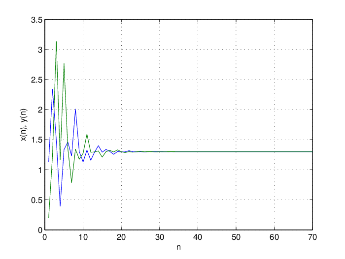
Example 2.

As an illustration of our results, we consider the following numerical example. Let $\alpha=2,\beta=3$ and $\gamma=5$ in system (2), then we obtain the system

x_{n+1}=\frac{2x_{n-1}+3}{5y_{n}x_{n-1}},\qquad y_{n+1}=\frac{2y_{n-1}+3}{5x_{n}y_{n-1}},\qquad n\in\mathbb{N}_{0}

(16)

Assume $x_{-1}=1.2,x_{0}=3.6,y_{-1}=2.3$ and $y_{0}=0.8.$ (See Fig. 2).

5 Summary and Recommendations

In this work, we have successfully established the closed-form solution of the rational difference equation

x_{n+1}=\frac{\alpha x_{n-1}+\beta}{\gamma x_{n}x_{n-1}}

as well as the closed-form solutions of its corresponding two-dimensional case

x_{n+1}=\frac{\alpha x_{n-1}+\beta}{\gamma y_{n}x_{n-1}},\qquad y_{n+1}=\frac{\alpha y_{n-1}+\beta}{\gamma x_{n}y_{n-1}}.

Also, we obtained stability results for the positive solutions of these systems. Particularly, we have shown that the positive solutions of each of these equations tends to a computable finite number, and is in fact expressible in terms of the well-known plastic number. Meanwhile, for future investigation, one could also derive the closed-form solution and examine the stability of solutions of the system

x_{n+1}=\frac{\alpha x_{n-1}-\beta}{\gamma y_{n}x_{n-1}},\qquad y_{n+1}=\frac{\alpha y_{n-1}\pm\beta}{\gamma x_{n}y_{n-1}}.

This work we leave to the interested readers.

References

[1] J. B. Bacani and J. F. T. Rabago, On linear recursive sequences with coefficients in arithmetic-geometric progressions, Appl. Math. Sci., 9(52) (2015), 2595-2607.
[2] L. Brand, A sequence defined by a difference equation, Am. Math. Mon., 62 (1955), 489-492.
[3] C. W. Clark, A delayed recruitement of a population dynamics with an application to baleen whale population, J. Math. Biol., 3 (1976), 381-391.
[4] B. M. M. De Weger, Padua and pisa are exponentially far apart, Publ. Mat., Barc., 41(2) (1997) 631-651.
[5] E. M. Elsayed, On a system of two nonlinear difference equations of order two, Proc. Jangeon Math. Soc., 18(3) (2015), 353-368.
[6] E. M. Elsayed and T. F. Ibrahim, Periodicity and solutions for some systems of nonlinear rational difference equations, Hacet. J. Math. Stat., 44(6) (2015), 1361-1390.
[7] E. M. Elsayed, Solution for systems of difference equations of rational form of order two, Comp. Appl. Math., 33(3) (2014), 751-765.
[8] G. Fulford, P. Forrester, A. Jones, Modelling with Differential and Difference Equations, Cambridge University Press, 12 June 1997.
[9] Y. Halim, Global character of systems of rational difference equations, Electron. J. Math. Analysis Appl., 3(1) (2015), 204-214.
[10] Y. Halim, Form and periodicity of solutions of some systems of higher-order difference equations, Math. Sci. Lett. 2, 5(1) (2016) 79-84.
[11] Y. Halim, A system of difference equations with solutions associated to Fibonacci numbers, Int. J. Difference Equ.,11( 1) (2016), 65-77.
[12] Y. Halim, N. Touafek and E. M. Elsayed, Closed forme solution of some systems of rational difference equations in terms of Fibonacci numbers, Dyn. Contin. Discrete Impulsive Syst. Ser. A, 21(5) (2014), 473-486.
[13] Y. Halim, N. Touafek and Y. Yazlik, Dynamic behavior of a second-order nonlinear rational difference equation, Turk. J. Math., 39(6) (2015), 1004- 1018.
[14] Y. Halim and M. Bayram, On the solutions of a higher-order difference equation in terms of generalized Fibonacci sequences, Math. Methods Appl. Sci., 39 (2016), 2974-2982.
[15] Y. Halim, J. F. T. Rabago, On some solvable systems of difference equations with solutions associated to Fibonacci numberss, Electron. J. Math. Analysis Appl., 5(1) (2017), 166-178.
[16] A. Khaliq and E. M. Elsayed, Qualitative properties of difference equation of order six, Mathematics, 4 (24) (2016), 14 pages.
[17] P. J. Larcombe and J. F. T. Rabago, On the Jacobsthal, Horadam and geometric mean sequences, Bull. Inst. Combin. Appl., 76 (2016), 117-126.
[18] R. E. Mickens, Difference Equations: Theory, Applications and Advanced Topics, 3rd ed. Chapman and Hall/CRC, 2015.
[19] A. G. Shannon, P. G. Anderson and A. F. Horadam, Properties of Cordonnier, Perrin and Van der Laan Numbers, Int. J. Math. Educ. Sci. Technol., 37(7) (2006), 825-831.
[20] J. F. T. Rabago, Effective methods on determining the periodicity and form of solutions of some systems of non-linear difference equations, Int. J. Dynamical Systems and Differential Equations, in press.
[21] J. F. T. Rabago, An intriguing application of telescoping sums, Proceeding of 2016 Asian Mathematical Conference, to appear.
[22] S. Stević, Representation of solutions of bilinear difference equations in terms of generalized Fibonacci sequences, Electron. J. Qual. Theory Differ. Equ., No. 67(2014), 1-15.
[23] S. Stević, On a system of difference equations, Appl. Math. Comput., 218(2011), 33723378.
[24] D. T. Tollu, Y. Yazlik, and N. Taskara, On the solutions of two special types of Riccati difference equation via Fibonacci umbers, Adv. Differ. Equ., 174 (2013), 7 pages.
[25] D. T. Tollu, Y. Yazlik and N. Taskara, The solutions of four Riccati difference equations associated with Fibonacci numbers, Balkan J. Math., 2 (2014), 163-172.
[26] D. T. Tollu, Y. Yazlik and N. Taskara, On fourteen solvable systems of difference equations, Appl. Math. & Comp., 233 (2014), 310-319.
[27] N. Touafek, On some fractional systems of difference equations, Iranian J. Math. Sci. Info., 9(2) (2014), 303-305.
[28] N. Touafek, On a second order rational difference equation, Hacet. J. Math. Stat., 41 (2012), 867-874.
[29] N. Touafek, On some fractional systems of difference equations, Iran. J. Math. Sci. Inform., 9(2) (2014), 73-86.
[30] N. Touafek and Y. Halim, Global attractivity of a rational difference equation, Math. Sci. Lett., 2(3) (2013), 161-165.
[31] N. Touafek and Y. Halim, On max type difference equations: expressions of solutions, Int. J. Nonlinear Sci., 11 (2011), 396-402.
[32] N. Touafek and E. M Elsayed, On the periodicity of some systems of nonlinear difference equations, Bull. Math. Soc. Sci. Math. Roum., Nouv. Sér., 55 (2012), 217-224.
[33] N. Touafek and E. M Elsayed, On the solutions of systems of rational difference equations, Math. Comput. Modelling, 55(7) (2012), 1987-1997.
[34] Y. Yazlik, D. T. Tollu and N. Taskara, On the solutions of difference equation systems with Padovan numbers, Appl. Math., J. Chin. Univ., 4(12) (2013), 15-20.