On the spectra of Pisot-cyclotomic numbers
Abstract.
We investigate the complex spectra
where is a quadratic or cubic Pisot-cyclotomic number and the alphabet is given by along with a finite collection of roots of unity. Such spectra are discrete aperiodic structures with crystallographically forbidden symmetries. We discuss in general terms under which conditions they possess the Delone property required for point sets modeling quasicrystals. We study the corresponding Voronoi tilings and we relate these structures to quasilattices arising from the cut and project method.
1. Introduction
Since the discovery of quasicrystals [19], it has been recognized the need of using irrational numbers in describing mathematical models of these aperiodic structures with non-crystallographically forbidden symmetries. The most common example are quasicrystals revealing five-fold (or ten-fold) symmetry, for which a model based on the golden ratio is required, see e.g. [14]. Quasicrystals with symmetry of order 8 and 12 correspond to other quadratic irrationalities. Only recently, quasicrystals with cubic irrationality have been observed [6], see also [20]. Naturally, rotation symmetries are connected to the so-called Pisot-cyclotomic numbers, whose most simple example is the golden ratio, and the quadratic and cubic cases are connected precisely to symmetries of order 5 (10), 7 (14), 8, 9 (18), and 12.
In [4], a convenient tool for studying quasicrystals has been identified, namely number representation in systems with irrational base. Although such non-standard number systems have been studied long before [18], their connection to quasicrystal models has only been exploited in recent years. In this paper we study originally a number-theoretic object, the so-called spectrum of a number. By its nature, the spectrum is self-similar and has a rotational symmetry. We demonstrate the utility of these structures for modelling quasicrystals.
The problem of the so-called spectrum of a real number has been introduced by Erdös et al. [5]. The spectrum of for is the set of polynomials with non-negative integer coefficients in the alphabet , evaluated in , . Specific properties are valid if is taken to be a Pisot number, i.e. an algebraic integer with conjugates smaller than in modulus. In particular, there is only a finite number of distances between consecutive points of , and the distance sequence can be generated by a substitution [7]. A generalization of the spectra to the complex plane was considered by Hejda and Pelantová [10], who define the spectrum of a complex Pisot number and study its Voronoi tessellation for the case of cubic complex Pisot units.
We consider a generalization in another direction. The base remains a real number , but the alphabet of digits is taken to be a finite set of complex numbers. In particular, we study the cases leading to as subsets of cyclotomic integers, providing thus discrete aperiodic structures with crystallographically forbidden symmetries. We focus on the cases where is a quadratic and cubic Pisot-cyclotomic number and the alphabet is formed by the origin and the vertices of a regular polygon.
Recall a Pisot number is a real algebraic integer such that all of ’s Galois conjugates are strictly less than in absolute value. A Pisot-cyclotomic number of order is a Pisot number such that . Notice that if is a Pisot-cyclotomic number of order , then will have degree , where is the Euler totient function. In the case when or , this means that is quadratic. In the case when or this means that is cubic. We list the set of all quadratic and cubic Pisot-cyclotomic numbers, in Table 1.
| order | name | approximate value | minimal polynomial |
|---|---|---|---|
| 5 or 10 | 1.618033989 | ||
| 2.618033989 | |||
| 7 or 14 | 2.246979604 | ||
| 4.048917340 | |||
| 5.048917340 | |||
| 20.44264896 | |||
| 21.44264896 | |||
| 8 | 2.414213562 | ||
| 3.414213562 | |||
| 9 or 18 | 2.879385242 | ||
| 7.290859369 | |||
| 8.290859369 | |||
| 12 | 2.732050808 | ||
| 3.732050808 |
Pisot-cyclotomic numbers of order play a crucial role in models for quasilattices and quasicrystals. The standard method used for such models is the cut-and-project method. In this paper we present an alternate model that comes from the spectra of a Pisot-cyclotomic number with respect to a specific digit set. We show that this alternate model shares many of the desired properties with the cut-and-project method. In some cases the two models coincide exactly, whereas in other we can show that these are two distinctly different models. Thus, we give an alternative model that may find future applications.
For a subset to be a quasilattice, one usually requires a number of specific properties.
- (i)
Rotational symmetry: For a root of unity, one has .
- (ii)
Dilation: There exists a , such that .
- (iii)
Uniform discreteness: There exists such that for all either or .
- (iv)
Relative density: There exists an such that for all we have .
- (v)
Finite local complexity: is uniformly discrete, relatively dense, and for each , the intersection of the set with the open ball is finite.
Sets satisfying properties (iii) and (iv) are called Delone sets. The supremum of parameters gives the double of the packing radius of , and the infimum of all with the required property is called the covering radius of ; we denote it by . Property (v) in fact means that there are only finitely many local configurations of any given radius. The closest neighbourhoods of points in a Delone set can be described using the so-called Voronoi tiles. A Voronoi tile of a point is the set of points in closer to than to any other point of . Voronoi tiles of all points of form a tiling of . If has property (v), the corresponding tiling is composed of copies of only finitely many Voronoi tiles.
All the (not necessarily primitive) -th roots of unity form vertices of a regular -gon in the complex plane, let us denote by them . We will consider the following sets,
This is the spectra of with respect to the alphabet . Note that by definition, we trivially have rotational symmetry as . We further see that we have dilation, as . In fact even strong is true, for any with one can show that . Hence this satisfies dilations with multiple possible centers. In Section 2 we discuss this set with respect to the other desired properties.
We show under what conditions gives a quasilattice satisfying properties (i)–(v). We will compare the corresponding spectrum with the cut-and-project sets defined for these cases. It turns out that sometimes, the acceptance window is given by a polygon, in other situations, we need to consider cut-and-project sets whose acceptance window have fractal boundary. Note that such structures appeared already in [1] in connection to aperiodic tilings. We also provide some information about the Voronoi tiling of the spectrum.
2. Uniform discreteness and relative density of the spectrum
By a variation of the Proof of Theorem 2.9 of Ngai and Wang [15] one can show that the spectrum of a Pisot number with alphabet being a finite subset of an imaginary quadratic extension of is always a uniformly discrete set.
Theorem 2.1.
Let be a Pisot number and let be a zero of a quadratic polynomial with negative discriminant. If is a finite alphabet, then the set is uniformly discrete.
Proof.
Let first be a finite set of integers. A well known property of Pisot numbers is that is uniformly discrete. See for example [8]. It is not hard to see that this is still true if we take with . For if with , then one can find an integer alphabet (consisting of sums of ) such that
Consider a finite set . Since is quadratic over , every element in can be written as where . Considering and we see that
As the polynomial has negative discriminant, is complex and therefore the right hand side of the above is a lattice composed of two uniformly discrete subsets of (one of them rotated by ). We see that the right hand side is uniformly discrete. Hence so is the left hand side as required. ∎
We see that Theorem 2.1 can be applied in the case of the spectrum of Pisot numbers under consideration.
Corollary 2.2.
Let be a Pisot-cyclotomic number of order , let be a primitive -th root of unity. If is a finite set, then the spectrum is uniformly discrete.
Proof.
We have , which implies that is a zero of the quadratic polynomial . By definition of Pisot-cyclotomic numbers, , thus is a polynomial over . Its discriminant is negative (except for that corresponds to the trivial case ). Thus we can apply Theorem 2.1 to obtain the result. ∎
Corollary 2.3.
Let be a Pisot-cyclotomic number of order and let be a finite set. If is relatively dense, then it is of finite local complexity.
Proof.
We need to check whether has finitely many elements in the ball of any radius . Since and , we can use Corollary 2.2 to obtain the statement. ∎
Under the assumption that is discrete, we can compute all the points of the finite set . The following algorithm is based on the observation that if such that , then
- •
Set and .
- •
Compute .
- •
Set .
- •
Repeat until
Let us concentrate on the question about relative density of the spectra in the complex plane. We provide a number of results for general real base and general complex alphabet. The next is an adaptation of Theorem 1.1 [10], where spectrum of complex numbers with an alphabet of integer digits is considered.
Theorem 2.4.
Let and let be finite. If , then is not relatively dense.
Proof.
Denote . For any relatively dense set , we have
| (1) |
Set . We will show that such does not satisfy (1). First notice that for any we have
which then clearly implies that
| (2) |
Indeed, consider with and such that . Then and . Since , the inclusion is valid.
The condition for relative density in Theorem 2.4 is necessary, but not sufficient. We further provide necessary and sufficient conditions for relative density of the spectrum in terms of representation of complex numbers in base with digits in .
Given a base and a finite alphabet , we will say that is -representable, if for any , there exists a convergent series
which is said to be a -representation of . For the given representation of , we define its integer and fractional parts,
For define the set as follows:
| (4) |
Remark 2.5.
It can be shown that is a compact set. In fact, it is the attractor of the iterated function system (IFS) with contraction and offsets . In particular, is the unique non-empty compact set satisfying
Proposition 2.6.
Let and let be finite. If is -representable, then is relatively dense. Moreover, for its covering radius, we have , where .
Proof.
By assumption, for any we have an expansion , . Let . Then and . ∎
In order to present an opposite statement, we need an additional requirement. Recall that we say a set is discrete, if for every , the intersection is finite.
Proposition 2.7.
Let and let be finite. If is relatively dense and discrete, then is -representable.
Proof.
Since is relatively dense, we can find, for a given , an element such that , where is the covering radius of . Similarly, we find a sequence such that for each , we have . Obviously, . We have to prove the existence of a series representing .
Since , we can write
Note that and is compact, thus we can find a subsequence of such that is convergent with .
Also the sequence is convergent. Since is discrete, is eventually constant, i.e. for .
Altogether, is a -representation of . ∎
Proposition 2.8.
Let and let be finite. Suppose that is discrete. Then is -representable if and only if .
Proof.
First suppose that , and consider . Necessarily, there exists such that . Therefore for some , whence has a -representation .
Suppose on the other hand that every has a -representation. If , then for its fixed representation we have
where , . Therefore the set is finite and its elements can be picked from for some fixed . This proves that all elements in have a representation with the integer part being . That is , i.e. . ∎
Theorem 2.9.
Let and be finite. Suppose that is discrete. Then the following statements are equivalent.
- (1)
is relatively dense.
- (2)
is -representable.
- (3)
.
- (4)
for every and .
3. Spectrum with polygonal alphabet
Let us focus on the specific example of the spectrum, namely when is a Pisot-cyclotomic number of order and the alphabet of digits is formed by the vertices of the regular -gon and the origin. In particular, . Recall we have denoted with . Since , it follows from Theorem 2.1 that the spectrum is uniformly discrete. Based on Theorem 2.4, the only options for relatively dense spectrum among the quadratic and cubic Pisot-cyclotomic numbers from Table 1 are (with and ), (with ), (with and ), (with ), (with and ), and (with ).
In order to prove/disprove relative density, we use Propositions 2.6 and 2.7, and the results of Herreros [11]. In his thesis, he considers representations of complex numbers in a real base with polygonal alphabet. In particular, he proves the following statement, which we rephrase with our notation.
| order | base | approx. value | relative density | ||
|---|---|---|---|---|---|
| 5 | 1.618033989 | 1.618033989 | YES | ||
| 10 | 1.618033989 | 2.618033989 | YES | ||
| 2.618033989 | 2.618033989 | YES | |||
| 7 | 2.246979604 | 2.246979604 | YES | ||
| 14 | 2.246979604 | 2.801937736 | YES | ||
| 8 | 2.414213562 | 2.414213562 | YES | ||
| 9 | 2.879385242 | 2.822714843 | NO | ||
| 18 | 2.879385242 | 2.879385242 | YES | ||
| 12 | 2.732050808 | 2.732050808 | YES |
Proposition 3.1.
Let and let . If , then is -representable. On the other hand, if for odd, or for even, then is not -representable.
It is important to notice that for our quadratic and cubic Pisot-cyclotomic numbers one has
This allows one to combine easily Proposition 2.6 with the statement of Herreros to obtain that all cases of the spectra are relatively dense, except the case that and . Here, one must check that
and thus Proposition 2.7 gives that the spectrum is not relatively dense. The results are summarized in Table 2.
In order to put these results in context of Proposition 2.8, see Figure 1 where the set is drawn for the considered cases.


4. Spectra and cut-and-project sets
Before starting our discussion on the connection of the spectra to cut-and-project sets, let us first review some of the basic details concerning the cut-and-project method. Usually, it is defined by projection of a section of a higher dimensional lattice to a suitably chosen subspace, see [13]. The cut-and-project scheme is given by two subspaces , of a -dimensional euclidean space , such that , , . Denote by (resp. ) the projection of to along (resp. along ). Given a lattice , we require that restricted to is injective, and that is dense in . Then, one has a mapping . If is a bounded subset of with non-empty interior, then we define .
In special cases leading to non-crystallographic symmetries, this definition can be recast in an algebraic way, in particular, with the use of Pisot-cyclotomic numbers [14]. We present here the definition of a cut-and-project set in this restricted frame, suitable for our purposes.
Let be a Pisot-cyclotomic number of order , and let be an -th root of unity. If is quadratic, there exists an automorphism of that takes to its conjugate . For cubic, there exist two different automorphisms and of that take to its two conjugates and , respectively.
It is worth observing that as and is totally real, then so is . It can be easily shown that . In particular, is equal to the ring of integers in the cyclotomic field . Set . It holds that and that is closed under Galois conjugation. Given a bounded set ( for quadratic , or for cubic ) with non-empty interior, we define the cut-and-project set by
for quadratic and
for cubic . The set is called the acceptance window. As the sets fall within the frame of model sets studied in [13], one can derive that such cut-and-project are uniformly discrete relatively dense sets of finite local complexity.
Sometimes, one considers cut-and-project sets where the acceptance window satisfies some additional properties. In our frame, taking symmetric under rotation of order , i.e. , we also have , which means that has -fold symmetry.
It is useful to consider also restriction of the above defined cut-and-project sets to one dimension, in this case presented as the cut-and-project sequence
amounts to the Galois conjugation in the field . The set is usually taken to be a bounded non-degenerated interval. Such sequences have been well described, in particular, they are easy to generate, and allow to generate more-dimensional cases, as we shall use further in this section.
Let us study whether the spectrum can be related to a cut-and-project set in the above setting. Obviously, a subset of the set of cyclotomic integers . It is natural to ask whether there exists a reasonable such that . We consider the Galois conjugation of elements of .
Theorem 4.1.
Let be a Pisot cyclotomic number of order and let . Suppose that is a Galois conjugation on such that . Then
Moreover, if contains in its interior, then
Proof.
Since , elements of are of the form , for , . Setting , we have . This implies . For the opposite inclusion, take , i.e. . Obviously is the limit of .
For the latter inclusion, it suffices to see the equivalence in Theorem 2.9. ∎
Corollary 4.2.
Since is the attractor of the corresponding IFS, one can derive some information about the shape . In particular
- •
If then is a polygon.
- •
If and is even then is a polygon.
- •
If and is odd then is a polygon.
The shapes of for all the quadratic resp. cubic cases are displayed in Figures 3 and 2. Note that if is a quadratic unit, we have . Thus when either and/or is even (which means ). In fact, the cases where this is not true are , and , (compare Figures 1 and 3).
From Theorem 4.1, one can derive a suitable choice of the acceptance window for comparing the spectra with cut-and-project sets.
Remark 4.3.
Let be a quadratic or a cubic Pisot-cyclotomic number of order and let . Then , where
In the quadratic case, we denote the Galois conjugation on such that . In the cubic case, we have similarly , .


In general, it is not easy to decide, whether all points of the cut-and-project set mentioned in Remark 4.3 are included in the spectrum, in other words, whether equality holds in . One way to verify this is to consider a criterion, which reduces the question to compare these sets only in a close neighbourhood of the origin. This task can be performed in few steps, taking into account that we have an algorithm to generate the spectra and cut-and-project sets. In order to decide whether there are some missing points (i.e. points in ) we start with the following lemma.
Lemma 4.4.
Let be a unit and let satisfy
| (5) |
Then implies .
Proof.
Let , i.e. By the assumption there exists such that Thus Note that the assumption that is a unit is used here to ensure that If , then also . We have that unless . Thus, by iterating this procedure, we eventually obtain a point in . ∎
Let us explain the consequences of this lemma in the quadratic case. The cubic case can be treated accordingly. Setting , the condition (5) is satisfied, even with equality. This has the following consequence.
Corollary 4.5.
Let . If is an algebraic unit, then the following are equivalent.
- (1)
- (2)
.
In the cases , , and we can apply Lemma 4.4 also to to be able to compare the sets and in those cases. We only need to show that such satisfies condition (5). This is easy to prove in case as is the open decagon. In cases and , things are more difficult, and we provide only a sketch of the proof for .
Let for any . Let be the closed decagon with vertices with as in (8). For we define . Then , thus , where the limit is with respect to the Hausdorff metric in the space of compact sets.
One can show that , thus we can find an open set such that . Define and . We see that is an open set in whose closure is . Moreover, it holds that , i.e. satisfies condition (5).
It is also possible, but rather technical to show that the Hausdorff distance of and tends to zero which implies that . As a byproduct we also obtain that is simply connected as each is simply connected.
A similar argumentation can be used to show that satisfies (5).
Corollary 4.6.
Let for and , and for and . Then the following are equivalent.
- (1)
- (2)
.
Corollaries 4.5 and 4.6 give us a technique to find all missing points. First step is to find all missing points such that . Next we check which of the points , , are missing, and we repeat this procedure.
Let us explain the method of finding the missing points of small absolute value. We need to compare the spectrum and the cut-and-project set in the ball . Finding all points of the spectrum within a bounded ball around the origin is straightforward using the techniques explained before. Let us focus on the method of generating all points of within a bounded region. For that, observe the trivial property of cut-and-project sets that
Thus, we choose a suitable for which the computation of is simple, and then we check which of its elements belong also to by verifying the condition on its conjugates. We set to be a parallelogram along the roots of unity, so that the cut-and-project set is a Cartesian product of two one-dimensional cut-and-project sequences .
Consider , where is a suitable interval. Then
By the above corollaries, we only need to consider points in , which amounts to finding points in , where is an interval such that . Then
In order to find all elements of , realize that these are of the form , , such that
This is a system of two linear inequalities for two unknowns , which can be easily solved.
Let us find explicitly the suitable intervals , for the considered cases. We have that is contained in with . Furthermore, is contained in the parallelogram with where . Similarly, we can set where . The appropriate choices of are shown in Table 3 together with intervals and . Figure 3 illustrates the acceptance windows with the missing points marked.
| order | missing points | ||||
|---|---|---|---|---|---|
| 5 | interior | ||||
| 10 | boundary | ||||
| boundary | |||||
| 8 | none | ||||
| 12 | interior |


Let us briefly explain how to decide whether given belongs to . This amounts to checking whether , i.e. whether there is a sequence of digits such that . For define . It is reasonable to consider only those digits such that . We claim that under the assumption that is an algebraic integer, if , , are such that , then takes only finitely many values. This fact can be shown in the same fashion as Lemma 9 of [2].
As a consequence, either there is no infinite sequence of digits such that , for each , and hence . Or, it happens that
and then we have that belongs to , and, moreover, it has an eventually periodic representation in powers of with preperiod and period . Therefore checking if can be done in a finite time even if has a fractal boundary.
For the case of symmetry of order 12, we consider the Pisot-cyclotomic number , which is not a unit. Hence we cannot apply Lemma 4.4, and consequently the corollaries. Nevertheless, we can decide that for , since already in the ball there are missing points, as it is seen from Figure 3e.
Similar procedure as in the quadratic case can be performed for the cases of cubic spectra, where both considered numbers are units. It turns out that none of the relatively dense cubic spectra corresponds to a cut-and-project set with simply connected acceptance windows, since there are many missing points. This is the reason we do not include the details of the computation.
5. Spectra and their Voronoi tilings
Let us focus on the Voronoi tiling of the spectrum. Such a tiling is important, for it provides a natural definition of ‘neighbours’ of points in an aperiodic Delone set. Formally, the Voronoi tile of a point in a Delone set is defined as
It is not difficult to see that only the closest points of influence the shape of the tile . In fact, one needs to look only to the distance , where is the covering radius of . The smallest finite subset such that
can be considered as the set of neighbours.
Consider a central point and additional points which surround . Between each and there is a line dividing such that each point on this line has equal distance from and . These lines form the boundary of the tile centered at . One can naturally define the neighbours of in as those points , whose tiles share a line segment with .
Denote the vertices of the tile by where each depends only on , and . As is the circumcenter of the triangle and we have that . Note that the disc of radius centered at contains no elements of in its interior. Therefore .
The maximal distance will be called the radius of the tile and denoted by . It is not difficult to realize that taking the supremum of radii of tiles over all points of , we obtain the covering radius of ,
| (6) |
If the set has finite local complexity, the supremum is achieved, i.e. there exists a tile whose radius is equal to .
An upper bound on the covering radius of the spectra was given in Proposition 2.6. In this section, we will find the exact value for for all our cases of the spectra of Pisot-cyclotomic numbers which are Delone. This will further allow us to provide a bound on the number of tiles in the corresponding tiling. In several cases, a more thorough inspection of the problem will allow us to determine the number of tiles precisely, see Section 6.
To find a lower bound on , simply compute the spectrum in some large neighbourhood of the origin, together with its Voronoi tiling, and find the maximum radii of these tiles. Computing an upper bound is more challenging, but still feasible. We will find an upper bound on by inspecting the radius of certain tiles in the tiling created by the (finite) set . Obviously, there are unbounded tiles at the boundaries, however, we will check only tiles in a suitable region around the origin.
Let be a subset of that is constructible by polynomials up to degree ,
Obviously, can be constructed by a union of translates of copies of , namely
For , consider regions , satisfying
| (7) |
It can be shown that we can set , where is given by the formula
| (8) |


Such a set has the following advantage for our computation. Take a point which belongs to . Then there exists an such that . Therefore one has a corresponding point such that .
Consider the Voronoi tile of the point created by points of . Then the Voronoi tile of the point is created by points , which lie in , and, perhaps, some additional points of . The Voronoi tile of with respect to is therefore cut from the Voronoi tile of with respect to . Consequently, the radius of is smaller or equal to the radius of , which, in turn, is bounded from above by the maximum of radii of tiles in the tiling of centered in points of . We denote this maximum by . We have thus demonstrated the following statement.
Corollary 5.1.
Let be the maximum of the radii of tiles in the tiling of centered at points in . Then is a decreasing sequence such that as tends to infinity.
Moreover, as is of finite local complexity, there exists some such that for all .
By inspecting tiles in the tiling of , , one obtains a sequence of upper estimates of the covering radius of . In our computation, we were successful, after a few steps, in obtaining an upper bound on which coincides with the lower bound obtained as explained earlier. Thus, we have derived the exact value of the covering radius for all our cases. The values of of the spectra of quadratic and cubic Pisot-cyclotomic numbers are, together with such that , displayed in Table 4.
| Symmetry | |||||
|---|---|---|---|---|---|
| 5 | 1.6180339895 | .7639320250 | 6 | ||
| 10 | 1.6180339895 | .6498393940 | 3 | ||
| 1.3763819202 | 1.051462225 | 1 | |||
| 7 | 1.2469796034 | 1.109916265 | 1 | ||
| 14 | 1.2469796034 | 1.025716864 | 1 | ||
| 8 | 1.3065629649 | 1.082392201 | 1 | ||
| 18 | 1.4619022000 | 1.015426612 | 1 | ||
| 12 | 1.4142135622 | 1.035276182 | 1 |
Remark 5.2.
It can be checked that, in fact, the covering radius of the spectrum is in all our cases equal to the radius of the Voronoi tile of the origin.
6. Local configurations
In a Delone set with finite local complexity, it is interesting to determine the number of local configurations of a given size. In the most restricted form of this question, we are interested in the number of different Voronoi tiles. Since a tile is given by a configuration of points within the distance at most , we immediately have that the Voronoi tiling is composed of translates of at most tiles. Clearly, this estimate is not reasonable. The bounds on the number of prototiles in the Voronoi tiling of the spectra can be improved by inspecting the local configurations of a given size. This method can be quite computationally expensive, but it yields also the shapes of the appearing tiles. At least in certain cases, we provide a complete description of the tiles in the Voronoi tiling, see Table 5.
Consider and define its local configuration as
We will say that two local configurations are equivalent if one is a rotation, or reflections of the second.
There are two key ideas about local configurations that are important:
Claim 6.1.
The Voronoi tile of is completely determined by the points in .
This observation follows from (6) and the upper bound on the covering radius obtained in Proposition 2.6.
Claim 6.2.
If for some and , then the local configuration of can be completely determined from the local configuration of .
Proof.
To see the second fact, we need to show that if is in of , then we can write for some and such that belongs to . This is easy to verify: As , there exist , such that . We have
from which we can derive that
Therefore , as required. ∎
We observe that for and , and hence one could consider local configurations of smaller radius than in these two cases.
It follows that local configurations of all points are in this sense descendants of the local configuration of the origin. This suggests the following algorithm for computation of all local configurations in the spectrum .
- •
Start with .
- •
From , compute for the local configuration as a set of those points in , that are in distance from .
- •
Repeat this process until finding the complete family of local configurations in the spectrum. The procedure must stop, since is of finite local complexity.
Example 6.3.
For example for and the local configuration of is . In fact, up to equivalents (rotation/reflection), there are 20 different local configurations. The algorithm described above gives rise to the diagram illustrated in Figure 5. These 20 local configurations generate only five distinct tiles.
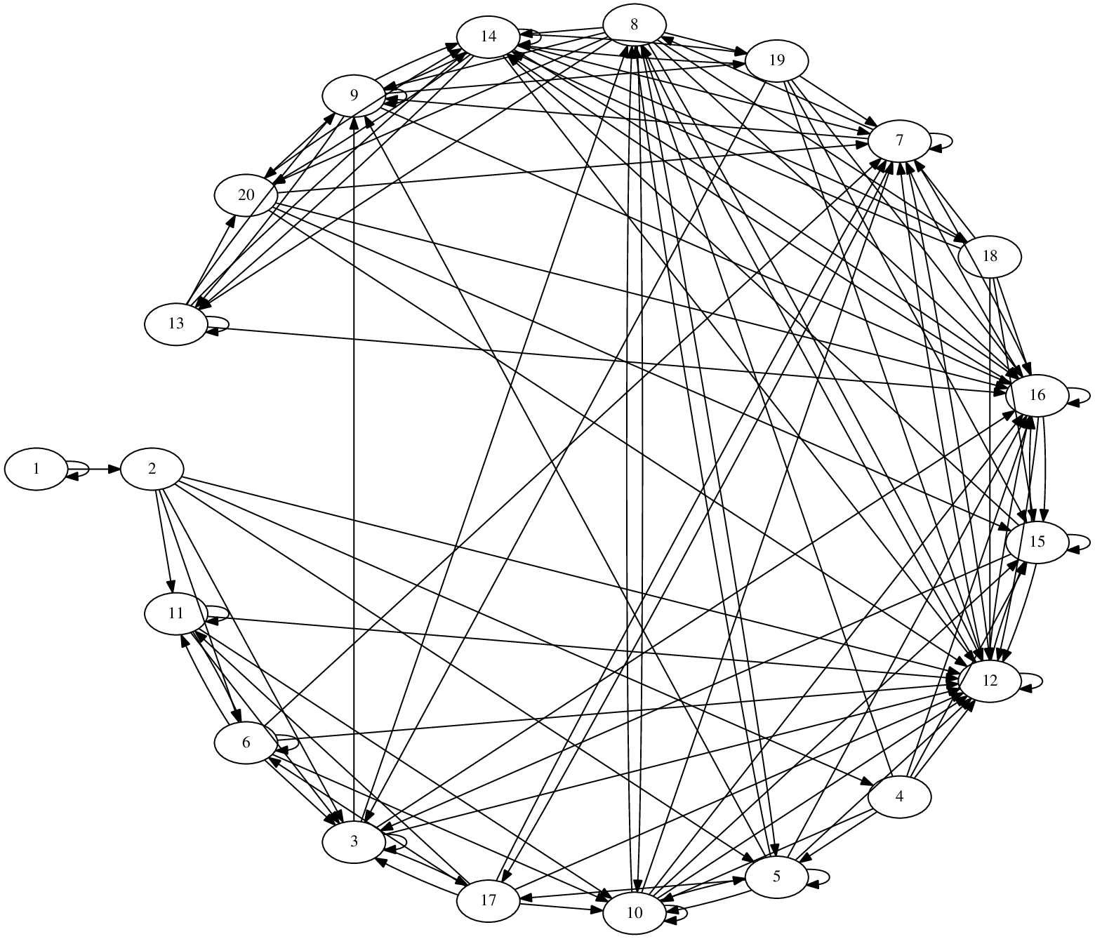
Table 5 shows the results of computations of local configurations in the considered cases of spectra of Pisot-cyclotomic numbers. Together with the number of local configurations we provide also the number of non-equivalent Voronoi tiles that these configurations generate. It turns out that only symmetry 5, 10, and 8 gives rise to ‘reasonable’ tilings with low number of different prototiles.
| Symmetric | Number of configurations | Number of tiles | |
|---|---|---|---|
| 5 | |||
| 10 | |||
| 10 | |||
| 7 | |||
| 14 | |||
| 8 | |||
| 18 | |||
| 12 |
7. Voronoi tilings for the quadratic and cubic cases
Let us summarize the knowledge about the spectra in individual cases of quadratic and cubic Pisot-cyclotomic numbers. We will consider only the cases which lead a relatively dense set, as given in Table 2.
In Section 6, we have provided a method for finding prototiles forming the Voronoi tiling of the spectra. In cases of symmetry 12, 7, 14 and 18, we have shown that the corresponding tilings are rather complex, with the number of shapes of prototiles exceeding a hundred. On the other hand, for symmetry 5 (), 10 (, ) and 8 (), our method yielded a complete list of prototiles. Moreover, the spectra , and also have the interesting property, that they correspond to a cut-and-project set with simply connected acceptance window, Therefore, one can consider easily the relation of the shape of the Voronoi cell of to the position of the image of in the acceptance window. These are quadratic cases, where, by Theorem 4.1, , denoting the unique automorphism of with non-trivial action on .
Suppose that the Voronoi cell of is given by the neighbours of . We have , . All points such that , , will either have the same type of Voronoi cell, or their Voronoi cell will be just a ‘cut’ of . Therefore the acceptance window will be divided into regions corresponding to prototiles, such that for any in a given region, has the corresponding tile as its Voronoi cell. These regions are bounded by intersections of the boundary of several suitably shifted copies of . This phenomenon is illustrated in Figures 7, 8, and 9. On the other hand, Figure 6 shows that in case there are some missing points in the acceptance window, the situation is much more complicated.
7.1. Case ,
Consider , see Figure 3. In Section 4, we have seen that the spectrum with pentagonal alphabet does not correspond to a cut-and-project set with simply connected acceptance window, since there are points in , where . Nevertheless, the tiling of this case of spectra can be described, see Figure 6. Surprisingly, there are only 12 prototiles.


7.2. Case ,
Consider , see Figure 3. In Section 4, we have seen that setting , there are no missing points, i.e. the spectrum of with decagonal alphabet satisfies
Moreover, since , we can derive from Theorem 2.9 that points of do not lie on the boundary of , thus we conclude that
i.e. the acceptance window is an open decagon of radius .
The tiling of this case of spectra is illustrated in Figure 7. There are 5 prototiles. Let us mention that the tiling for for this case was already described in [12]. It can be shown that only 3 of the 5 prototiles appear with non-zero density in the tiling.


7.3. Case ,
Consider , see Figure 3. By a similar argumentation as for and , we can derive that this case of the spectra corresponds to a cut-and-project set with simply connected acceptance window which now has fractal nature. We have
The tiling of this case of spectra is illustrated in Figure 7. Again, there are 5 prototiles, four of which appear with non-zero density in the tiling. The decagonal tile appears only once.


7.4. Case ,
Consider , see Figure 3. Here,
| (9) |
This follows from
| (10) |
where the first inclusion uses the fact that , and item 4 of Theorem 2.9. Moreover, we know that due to Corollary 4.5.
It it surprising but true, that the inclusion or exclusion of the boundary makes no difference to the cut and project method in this case. This is because points on the boundary do not correspond to algebraic integers in . For example, the point on the real line with maximal absolute value is equal to .
The tiling of has exactly 5 distinct types of tiles, all of them appearing with non-zero density.


7.5. 12-fold symmetry
Consider (see Figure 3). In this case is not a unit, so Corollaries 4.5 and 4.6 do not apply, nevertheless, we have found points in , which means that this case of the spectra does not correspond to a cut-and-project set with simply connected acceptance window. This fact also reflects in that the tile set of this spectrum contains over hundred distinct types of tiles.
7.6. 7-, 14- and 18-fold symmetry
Consider the candidates for the acceptance windows, according to Remark 4.3 and Figure 2. By an analysis similar to that for quadratic cases, we derive that the spectrum cannot be identified with a cut-and-project set with reasonable acceptance window. Our computation shows that also the Voronoi tiling is complicated:
- •
has at least 201 distinct types of tiles.
- •
has at least 189 distinct types of tiles.
- •
has at least 154 distinct types of tiles.


Conclusions
In this paper we have studied the possibility to model quasicrystals with symmetries of order 5 (10), 7 (14), 8, 9 (18), 12 by spectra of Pisot-cyclotomic numbers of degree two or three. It turned out that in the quadratic case, there are spectra that can be identified with self-similar quasilattices defined by the cut-and-project scheme. Similar structures have been studied in [16], however, our approach uses techniques from non-standard number systems and thus brings a new insight into the question. For, the possibility to model certain quasilattices by cut-and-project sets with simply connected acceptance windows is closely related to representability of all complex numbers in an appropriate base with digits in a suitably chosen alphabet. Our results of number-theoretical nature are collected in Section 2 and are of independent interest.
Acknowledgements
This work was supported by the Czech Science Foundation, grant No. 13-03538S. We also acknowledge financial support of the Grant Agency of the Czech Technical University in Prague, grant No. SGS14/205/OHK4/3T/14. The Research of K. G. Hare was supported by NSERC Grant RGPIN-2014-03154.
References
- [1] M. Baake, R. Klitzing, M. Schlottmann, Fractally shaped acceptance domains of quasiperiodic square-triangle tilings with dedecagonal symmetry, Physica A: Statistical Mechanics and its Applications 191, Issues 14, (1992), 554–558.
- [2] S. Baker, Z. Masáková, E. Pelantová, T. Vávra, On periodic representations in non-Pisot bases, to appear in Monatshefte fur Mathematik (2016).
- [3] J.P. Bell, K.G. Hare, A classification of (some) Pisot-Cyclotomic numbers, J. Number Theory 115 (2005), 215–229.
- [4] C. Burdík, Ch. Frougny, J. P. Gazeau, R. Krejcar, Beta-integers as natural counting systems for quasicrystals, J. Phys. A: Math. Gen., 31, Number 30 (1998), 6449-6472.
- [5] P. Erdős, I. Joó, V. Komornik, Characterization of the unique expansions and related problems, Bull. Soc. Math. France 118 (3) (1990), 377–390.
- [6] A. Exner, S. Förster, S. Fischer, et al. Colloidal quasicrystals with 12-fold and 18-fold diffraction symmetry, PNAS, 108(5) (2011), 1810–1814.
- [7] D.-J. Feng, Z.-Y. Wen, A property of Pisot numbers, J. Number Theory, 97 (2) (2002), 305–316.
- [8] A. M. Garsia, Arithmetic properties of Bernoulli convolutions, Trans. Amer. Math. Soc. 102 (1962), 409–432.
- [9] L.-S. Guimond, Z. Masáková, E. Pelantová, Combinatorial properties of infinite words associated with cut-and-project sequences, J. Théor. Nombres Bordeaux 15 (2003), 697–725.
- [10] T. Hejda, E. Pelantová, Spectral properties of cubic complex Pisot units, Math. Comp. 85 (2016), no. 297, 401–421.
- [11] Y. Herreros, Contribution a l’arithmétique des ordinateurs, Ph.D. thesis, Institut polytechnique de Grenoble, 1991.
- [12] Z. Masáková, J. Patera, J. Zich, Classification of Voronoi and Delone tiles of quasicrystals III: decagonal acceptance window of any size, J. Phys. A: Math. Gen. 38 (2005), 1947–1960.
- [13] R. V. Moody, Model sets: A survey, in: From Quasicrystals to More Complex Systems, Centre de Physique des Houches Volume 13, (2000), 145–166.
- [14] R. V. Moody, J. Patera, Quasicrystals and icosians, J. Phys. A 26 (1993), no. 12, 2829–2853.
- [15] S.M. Ngai, Y. Wang, Hausdorff dimension of self-similar sets with overlaps, J. London Math. Soc., 63 (2001), 655–672.
- [16] K. Niizeki, Self-similar quasilattices with windows having fractal boundaries, J. Phys. A: Math. Theor., 41, Number 17, (2008), 175208.
- [17] K. Niizeki, A dodecagonal quasiperiodic tiling with a fractal window Phil. Mag. 87, Iss. 18-21, (2007), 2855–2861.
- [18] A. Rényi, Representations for real numbers and their ergodic properties, Acta Mathematica Academiae Scientiarum Hungaricae, 8: (1957), 477-493.
- [19] D. Shechtman, I. Blech, D. Gratias, J. W. Cahn, Metallic Phase with Long-Range Orientational Order and No Translational Symmetry, Phys. Rev. Lett. 53, (1984), 1951.
- [20] W. Steurer, Boron-based quasicrystals with sevenfold symmetry, Phil. Mag. 87, Iss. 18-21, (2007), 2707–2711.