In the $\Delta S=2$ observables, there are the indirect CP violation $\epsilon_{K}$ and the mass difference $\Delta m_{K}$ in the $K^{0}\textrm{--}\overline{K}{}^{0}$ mixing. Since $\epsilon_{K}$ has been measured precisely, and the SM prediction is accurate, it provides a severe constraint. The SM and NP contributions are shown as

where $\varphi_{\epsilon}=(43.51\pm 0.05)^{\circ}$. The NP contribution is given by the double penguin diagrams with the $Z$ boson exchange (Fig. 1 (a)),

where the right-hand side is [15]

In these expressions, renormalization group corrections and long-distance contributions are included [25]. In addition, one must take account of the interference terms between the SM and NP contributions (Figs. 1 (b)–(e)),

Here, the SM contribution, $\Delta_{L}^{\rm SM}$, is generated by radiative corrections.

At the one-loop level, it is calculated as

where $c_{W}=\cos\theta_{W}$, $\lambda_{i}\equiv V_{is}^{\ast}V_{id}$ with the CKM matrix $V_{ij}$, and $\mu_{\rm NP}$ corresponds to the NP scale.^#4#4 #4 In order to introduce how significant the interference contributions are, we ignore the renormalization group corrections to the dimension-6 operators above the electroweak scale except for a first leading logarithmic contribution $\ln(\mu_{\rm NP}/m_{W})$ which comes from Fig. 1 (e). This approximation is valid when the NP scale is not so far from the electroweak scale. In this letter, the CKMfitter result [24] is used for the CKM elements, unless otherwise mentioned. The loop function is^#5#5 #5 The loop function $\widetilde{C}(x,\mu_{\rm NP})$ is consistent with the result in Ref. [26].

In the Feynman-’t Hooft gauge, the first term in the right-hand side corresponds to the $Z$-boson exchange diagram [22] (Fig. 1 (b)),

while the second term is obtained from the Nambu-Goldstone boson loops (Figs. 1 (c)–(e)),

The explicit form of $\Delta C(x)$ depends on the effective operators above the electroweak symmetry breaking scale. Here, they are supposed to be $\mathcal{O}_{L}$ and $\mathcal{O}_{R}$. It is noted that the interference terms are gauge-independent.

The interference terms (2.8) have been overlooked in Refs. [22, 11, 15, 13]. They cannot be ignored, as we will see in the next section.

The latest estimation of the SM value is [27]

On the other hand, the experimental result is [10]

They are well consistent with each other, and $\epsilon_{K}^{\rm NP}$ must satisfy

at the $2\,\sigma$ level.^#6#6 #6 The SM estimation $\epsilon_{K}^{\rm SM}$ is sensitive to the CKM elements. If one uses $V_{cb}$ that is determined by the exclusive $B\to D^{(\ast)}\ell\nu$ decays [28], $\epsilon_{K}^{\rm SM}=(1.73\pm 0.18)\cdot 10^{-3}$ is obtained [29]. Then, $\epsilon_{K}^{\rm NP}=(0.50\pm 0.18)\cdot 10^{-3}$ is required at the $1\,\sigma$ level.

The kaon mass difference $\Delta m_{K}$ consists of the SM and NP contributions:

If we parameterize the NP contribution as

the right-hand side is estimated as [15]

Similarly to the case of $\epsilon_{K}$, there are interference terms between the SM and NP contributions,

Here, $\Delta_{L}^{\rm SM}$ is given by Eq. (2.9), and the result is gauge-independent. These terms have been overlooked in the literature.

The experimental result is [10]

Since the SM prediction involves sizable contributions of long-distance effects, the uncertainty is large.^#7#7 #7 The latest lattice simulation, which includes the long-distance contributions, provides $\Delta m_{K}^{\rm SM}=(3.19\pm 1.04)\cdot 10^{-15}\,{\rm GeV}$ [30]. However, it is performed on masses of unphysical pion, kaon and charmed quark. Hence, we simply require that the NP contribution does not exceed the experimental value (with the $2\,\sigma$ uncertainty):

This constraint will turn out to be much weaker than $\epsilon_{K}^{\rm NP}$.

The flavor-changing $Z$ interaction also contributes to $\Delta S=1$ observables. The direct CP violation $\epsilon^{\prime}/\epsilon$ is shown as

The NP contribution is estimated as [15]

where $B_{8}^{(3/2)}=0.76\pm 0.05$ from the lattice calculation. Here, the terms which are not proportional to $B_{8}^{(3/2)}$ are omitted; the approximation is valid at the 10 % accuracy. A factor in the parenthesis gives $c_{W}^{2}/s_{W}^{2}\simeq 3.33$. Thus, the NP contribution can be enhanced easily by $\Delta_{R}$.

As mentioned in Sec. 1, the SM prediction deviates from the experimental result at the $2.8$–$2.9\,\sigma$ level. In this letter, we require that the discrepancy of $\epsilon^{\prime}/\epsilon$ is explained at the $1\,\sigma$ level as

where Ref. [6] is used for the SM prediction.

The (ultra-)rare kaon decay channels, $K^{+}\to\pi^{+}\nu\bar{\nu}$ and $K_{L}\to\pi^{0}\nu\bar{\nu}$, are correlated with $\epsilon^{\prime}/\epsilon$ as well as $\epsilon_{K}$ and $\Delta m_{K}$ in the general $Z$ scenario.^#8#8 #8 The branching ratios of $K\to\pi\ell^{+}\ell^{-}$ ($\ell=e,\,\mu$) are also affected in the general $Z$ scenario. However, $K^{+}\to\pi^{+}\ell^{+}\ell^{-}$ and $K_{S}\to\pi^{0}\ell^{+}\ell^{-}$ are dominated by a long-distance contribution through $K\to\pi\gamma^{\ast}\to\pi\ell^{+}\ell^{-}$ [31]. On the other hand, such a contribution to $K_{L}\to\pi^{0}\ell^{+}\ell^{-}$ is forbidden by the CP symmetry, but is dominated by an indirect CP-violating contribution, $K_{L}\to K_{S}\to\pi^{0}\ell^{+}\ell^{-}$ [31]. Therefore, it is challenging to discuss shot-distance NP contributions in these channels. They are represented as [32, 15]

Here, $X_{\rm eff}$ is estimated as

where the first term in the right-hand side is the SM contribution. Also, $\lambda=|V_{us}|$, $\kappa_{+}=(5.157\pm 0.025)\cdot 10^{-11}(\lambda/0.225)^{8}$, and $\kappa_{L}=(2.231\pm 0.013)\cdot 10^{-10}(\lambda/0.225)^{8}$. The charm-quark contribution is $P_{c}(X)=(9.39\pm 0.31)\cdot 10^{-4}/\lambda^{4}+(0.04\pm 0.02)$, where the first term in the right-hand side comes from short-distance effects, while the second one takes account of long-distance effects. Using the CKMfitter result for the CKM elements, one obtains

The SM predictions become

On the other hand, the experimental results are [33, 34]

Although the current constraints on the NP contributions are very weak, the experimental values will be improved significantly in the near future. The NA62 experiment at CERN, which already started the physics run at low beam intensity in 2015, has a potential to measure $\mathcal{B}(K^{+}\to\pi^{+}\nu\bar{\nu})$ at the 10 % precision by 2018 [35]. The KOTO experiment at J-PARC is designed to improve the sensitivity for $\mathcal{B}(K_{L}\to\pi^{0}\nu\bar{\nu})$, which enables us to measure it at the 10 % level of the SM value [36, 37]. As one can see from Eqs. (2.23) and (2.27), the NP contributions to $\mathcal{B}(K\to\pi\nu\bar{\nu})$ are correlated with those to $\epsilon^{\prime}/\epsilon$ in the general $Z$ scenario. Thus, if the $\epsilon^{\prime}/\epsilon$ discrepancy is a signal of the scenario, these experiments would detect NP effects.

The branching ratio of $K_{L}\to\mu^{+}\mu^{-}$ is also sensitive to the NP contributions to the flavor-changing $Z$ couplings. Theoretically, only the short-distance (SD) contributions can be calculated reliably. They are shown as [38, 39, 15]

where $\kappa_{\mu}=(2.01\pm 0.02)\cdot 10^{-9}(\lambda/0.225)^{8}$. The charm-quark contribution is $P_{c}(Y)=(0.115\pm 0.018)\cdot(0.225/\lambda)^{4}$. Using the CKMfitter result, one obtains

where the first term in the right-hand side is the SM contribution, and the minus sign between $\Delta_{L}$ and $\Delta_{R}$ is due to the axial-vector current. The SM value is obtained as

On the other hand, it is challenging to extract a short-distance part in the experimental data $\mathcal{B}(K_{L}\to\mu^{+}\mu^{-})_{\rm exp}=(6.84\pm 0.11)\cdot 10^{-9}$ [10], because of huge long-distance contributions through $K_{L}\to\gamma^{\ast}\gamma^{\ast}\to\mu^{+}\mu^{-}$ [40]. An upper bound on the short-distance contribution is [40]

Since the constraint is much weaker than the SM uncertainties, we ignore them for simplicity and impose a bound on the $Z$ couplings,

The real parts of the NP contributions are constrained by $\mathcal{B}(K_{L}\to\mu^{+}\mu^{-})$.

First, we consider the following simplified scenarios (c.f., Ref. [41]),

• •

  left-handed scenario (LHS): $\Delta_{R}=0$,^#10#10 #10 This scenario is realized by chargino contributions to the $Z$ penguin in the supersymmetric model [42, 43, 44, 17, 19].

• •

  right-handed scenario (RHS): $\Delta_{L}=0$,^#11#11 #11 Randall-Sundrum models with custodial protection [45, 46] can generate large $\Delta_{R}$. However, there are additional effects, e.g., from KK-gluon diagrams for $\epsilon_{K}^{\rm NP}$.

• •

  pure imaginary scenario (ImZS): ${\rm Re}\,\Delta_{L}={\rm Re}\,\Delta_{R}=0$,

• •

  left-right symmetric scenario (LRS): $\Delta_{L}=\Delta_{R}$.^#12#12 #12 In axial-symmetric scenarios, $\Delta_{L}=-\Delta_{R}$, there are no NP contributions to $K\to\pi\nu\bar{\nu}$.

As shown below, these scenarios do not require large parameter tuning in $\epsilon_{K}^{\rm NP}$. However, $\mathcal{B}(K\to\pi\nu\bar{\nu})$ will turn out to be small.

In Fig. 2, the $Z$-penguin observables are shown as functions of $\Delta_{L,R}$ for LHS and RHS. In the green (light green) regions, the $\epsilon^{\prime}/\epsilon$ discrepancy is explained at $1\,(2)\,\sigma$. They depend only on the imaginary component of $\Delta_{L,R}$. Obviously, $\epsilon^{\prime}/\epsilon$ is enhanced by the right-handed $Z$ coupling, $\Delta_{R}$, more than $\Delta_{L}$.

The blue regions are excluded by the $\epsilon_{K}$, and the orange regions are by the $\mathcal{B}(K_{L}\to\mu^{+}\mu^{-})$. The constraint from $\epsilon_{K}$ is much severer in RHS than LHS due to the interference contributions, Eq. (2.8). There is no constraint from $\Delta m_{K}$ in the parameter regions of the plots.

The red and black dashed contours represent $\mathcal{B}(K_{L}\to\pi^{0}\nu\bar{\nu})/\mathcal{B}(K_{L}\to\pi^{0}\nu\bar{\nu})_{\rm SM}$ and $\mathcal{B}(K^{+}\to\pi^{+}\nu\bar{\nu})/\mathcal{B}(K^{+}\to\pi^{+}\nu\bar{\nu})_{\rm SM}$, respectively. Here and hereafter, $\mathcal{B}(K_{L}\to\pi^{0}\nu\bar{\nu})_{\rm SM}$ and $\mathcal{B}(K^{+}\to\pi^{+}\nu\bar{\nu})_{\rm SM}$ denote the central values of the SM predictions, Eqs. (2.30) and (2.31). It is found that $\mathcal{B}(K_{L}\to\pi^{0}\nu\bar{\nu})$ cannot be as large as the SM value as long as $\epsilon^{\prime}/\epsilon$ is explained in LHS or RHS. On the other hand, if the $\epsilon^{\prime}/\epsilon$ discrepancy is explained by LHS, the NP contribution to $\mathcal{B}(K^{+}\to\pi^{+}\nu\bar{\nu})$ is limited by $\mathcal{B}(K_{L}\to\mu^{+}\mu^{-})$. In contrast, $\epsilon_{K}$ restricts RHS.

Next, we consider ImZS. Such a situation is often considered to amplify $(\epsilon^{\prime}/\epsilon)_{\rm NP}$ but suppress $\epsilon_{K}^{\rm NP}$. In the left panel of Fig. 3, the $Z$-penguin observables are shown as functions of ${\rm Im}\,\Delta_{L,R}$. The most severe constraint is from $\epsilon_{K}$ due to the interference between the SM and NP. The other bounds are weak and absent in the plot. Since there are no real components of $\Delta_{L,R}$, $\mathcal{B}(K^{+}\to\pi^{+}\nu\bar{\nu})$ is correlated with $\mathcal{B}(K_{L}\to\pi^{0}\nu\bar{\nu})$.

Finally, LRS is shown in the right panel of Fig. 3. Similarly to the cases of RHS and ImZS, most of the parameter regions are excluded by $\epsilon_{K}$. The NP contributions to $\mathcal{B}(K_{L}\to\mu^{+}\mu^{-})$ vanish because the process is the axial-vector current.

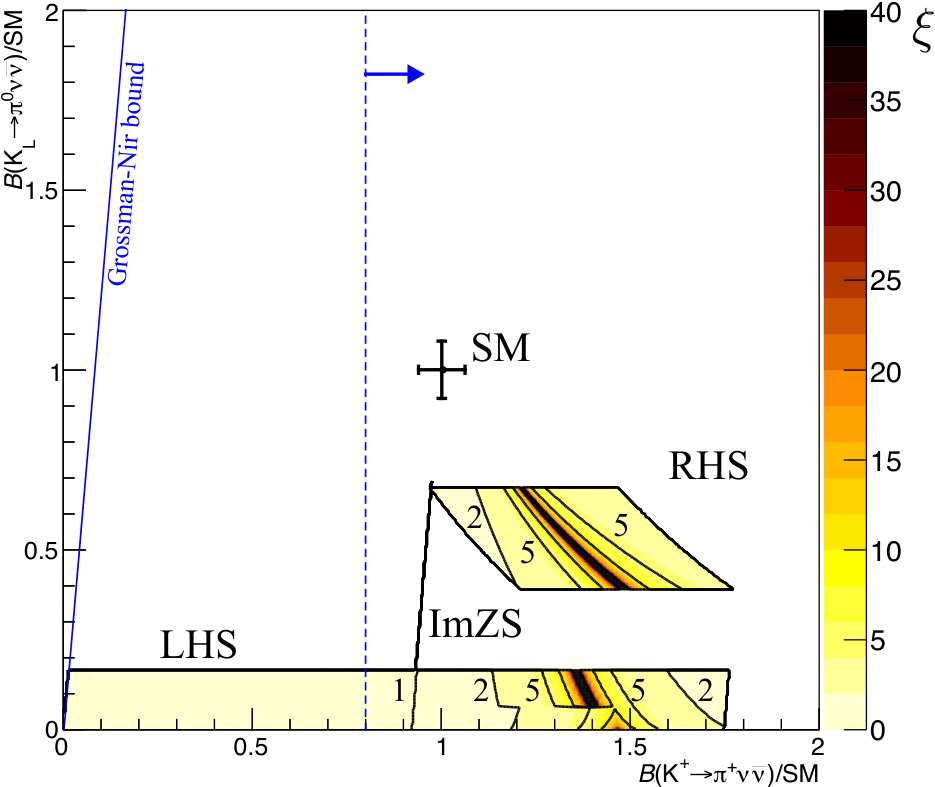
In Fig. 4, contours of the tuning parameter $\xi$ are shown for the simplified scenarios: LHS, RHS, ImZS, and LRS on the plane of the branching ratios of $K\to\pi\nu\bar{\nu}$. We scanned the whole parameter space of $\Delta_{L,R}$ in each scenario and selected the parameters where $\epsilon^{\prime}/\epsilon$ is explained at the $1\sigma$ level, and the experimental bounds from $\epsilon_{K}$, $\Delta m_{K}$, and $\mathcal{B}(K_{L}\to\mu^{+}\mu^{-})$ are satisfied (see the previous section for the experimental constraints). Then, $\xi$ was estimated at each point. Several parameter sets predict the same $\mathcal{B}(K^{+}\to\pi^{+}\nu\bar{\nu})$ and $\mathcal{B}(K_{L}\to\pi^{0}\nu\bar{\nu})$. Among them, the smallest $\xi$ is chosen in Fig. 4 for each set of $\mathcal{B}(K^{+}\to\pi^{+}\nu\bar{\nu})$ and $\mathcal{B}(K_{L}\to\pi^{0}\nu\bar{\nu})$. In most of the allowed parameter regions, $\xi=\mathcal{O}(1)$ is obtained. Thus, one does not require tight tunings in these scenarios.

In the figures, $\mathcal{B}(K_{L}\to\pi^{0}\nu\bar{\nu})$ is smaller than the SM value by more than 30%. Hence, the scenarios could be tested by the KOTO experiment. On the other hand, $\mathcal{B}(K^{+}\to\pi^{+}\nu\bar{\nu})$ depends on the scenarios. In LHS, we obtain $0<\mathcal{B}(K^{+}\to\pi^{+}\nu\bar{\nu})/\mathcal{B}(K^{+}\to\pi^{+}\nu\bar{\nu})_{\rm SM}<1.8$. In RHS, $\mathcal{B}(K^{+}\to\pi^{+}\nu\bar{\nu})$ is comparable to or larger than the SM value, but cannot be twice as large. In ImZS, the branching ratios are perfectly correlated and displayed by a line in Fig. 4. Then, $\mathcal{B}(K^{+}\to\pi^{+}\nu\bar{\nu})$ is not deviated from the SM one. The right panel of Fig. 4 is a result of the tuning parameter $\xi$ in LRS. It is found that $\mathcal{B}(K_{L}\to\pi^{0}\nu\bar{\nu})$ does not exceed about a half of the SM value. On the other hand, $\mathcal{B}(K^{+}\to\pi^{+}\nu\bar{\nu})$ is comparable to or larger than the SM value, but cannot be twice as large, as is similar to RHS.

Let us consider the full parameter space in the general $Z$ scenario. Both $\Delta_{L}$ and $\Delta_{R}$ are turned on. Then, $\mathcal{B}(K^{+}\to\pi^{+}\nu\bar{\nu})$ and/or $\mathcal{B}(K_{L}\to\pi^{0}\nu\bar{\nu})$ can be enhanced if the tuning for $\epsilon_{K}^{\rm NP}$ is allowed.

In Fig. 5, the branching ratios of $K\to\pi\nu\bar{\nu}$ and the tuning parameter are shown for the case of $(\epsilon^{\prime}/\epsilon)_{\rm NP}=15.5\cdot 10^{-4}$ and $\epsilon_{K}^{\rm NP}=0.37\cdot 10^{-3}$. The flavor-changing $Z$ couplings, and namely the NP contributions to $K\to\pi\nu\bar{\nu}$, are limited by $\mathcal{B}(K_{L}\to\mu^{+}\mu^{-})$ and the tuning parameter.

In Fig. 6, contours of the tuning parameter $\xi$ are shown on the plane of the branching ratios of $K\to\pi\nu\bar{\nu}$. The whole parameter space of the general $Z$ scenario is scanned. In the colored regions, $\epsilon^{\prime}/\epsilon$ is explained at the $1\sigma$ level, and the experimental bounds of $\epsilon_{K}$, $\Delta m_{K}$, and $\mathcal{B}(K_{L}\to\mu^{+}\mu^{-})$ are satisfied (see the previous section for the experimental constraints). For each set of $\mathcal{B}(K^{+}\to\pi^{+}\nu\bar{\nu})$ and $\mathcal{B}(K_{L}\to\pi^{0}\nu\bar{\nu})$, the smallest $\xi$ is chosen among the parameter sets which predict the same branching ratios.

Compared to the simplified cases in Fig. 4, $\mathcal{B}(K_{L}\to\pi^{0}\nu\bar{\nu})$ can be enhanced. The tuning parameter is not necessarily very large if only one of $\mathcal{B}(K_{L}\to\pi^{0}\nu\bar{\nu})$ and $\mathcal{B}(K_{L}\to\mu^{+}\mu^{-})$ is enhanced. However, $\xi\gtrsim 30$–$40$ is required to amplify both of them. If $\xi\lesssim 10$ (5) is allowed, $\mathcal{B}(K_{L}\to\pi^{0}\nu\bar{\nu})$ can be as large as $6\times 10^{-10}$ ($2\times 10^{-10}$). In other words, $\mathcal{O}(10)$% tunings are required to enhance $\mathcal{B}(K_{L}\to\pi^{0}\nu\bar{\nu})$ by an order of magnitudes compared the SM prediction. The KOTO experiment can probe such large branching ratios in the near future.

References

- [1] T. Blum et al., “The Decay Amplitude from Lattice QCD,” Phys. Rev. Lett. 108, 141601 (2012) [arXiv:1111.1699 [hep-lat]].
- [2] T. Blum et al., “Lattice determination of the Decay Amplitude ,” Phys. Rev. D 86, 074513 (2012) [arXiv:1206.5142 [hep-lat]].
- [3] T. Blum et al., “ decay amplitude in the continuum limit,” Phys. Rev. D 91, no. 7, 074502 (2015) [arXiv:1502.00263 [hep-lat]].
- [4] Z. Bai et al. [RBC and UKQCD Collaborations], “Standard Model Prediction for Direct CP Violation in Decay,” Phys. Rev. Lett. 115, no. 21, 212001 (2015) [arXiv:1505.07863 [hep-lat]].
- [5] A. J. Buras, M. Gorbahn, S. Jäger and M. Jamin, “Improved anatomy of in the Standard Model,” JHEP 1511, 202 (2015) [arXiv:1507.06345 [hep-ph]].
- [6] T. Kitahara, U. Nierste and P. Tremper, “Singularity-free Next-to-leading Order Renormalization Group Evolution and in the Standard Model and Beyond,” JHEP 1612, 078 (2016) [arXiv:1607.06727 [hep-ph]].
- [7] J. R. Batley et al. [NA48 Collaboration], “A Precision measurement of direct CP violation in the decay of neutral kaons into two pions,” Phys. Lett. B 544, 97 (2002) [hep-ex/0208009].
- [8] A. Alavi-Harati et al. [KTeV Collaboration], “Measurements of direct CP violation, CPT symmetry, and other parameters in the neutral kaon system,” Phys. Rev. D 67, 012005 (2003), Erratum: [Phys. Rev. D 70, 079904 (2004)] [hep-ex/0208007].
- [9] E. Abouzaid et al. [KTeV Collaboration], “Precise Measurements of Direct CP Violation, CPT Symmetry, and Other Parameters in the Neutral Kaon System,” Phys. Rev. D 83, 092001 (2011) [arXiv:1011.0127 [hep-ex]].
- [10] C. Patrignani et al. [Particle Data Group Collaboration], “Review of Particle Physics,” Chin. Phys. C 40, no. 10, 100001 (2016).
- [11] A. J. Buras, F. De Fazio and J. Girrbach, “ rule, and in and models with FCNC quark couplings,” Eur. Phys. J. C 74, no. 7, 2950 (2014) [arXiv:1404.3824 [hep-ph]].
- [12] M. Blanke, A. J. Buras and S. Recksiegel, “Quark flavour observables in the Littlest Higgs model with T-parity after LHC Run 1,” Eur. Phys. J. C 76, no. 4, 182 (2016) [arXiv:1507.06316 [hep-ph]].
- [13] A. J. Buras, D. Buttazzo and R. Knegjens, “ and in simplified new physics models,” JHEP 1511, 166 (2015) [arXiv:1507.08672 [hep-ph]].
- [14] A. J. Buras and F. De Fazio, “ in 331 Models,” JHEP 1603, 010 (2016) [arXiv:1512.02869 [hep-ph]].
- [15] A. J. Buras, “New physics patterns in and with implications for rare kaon decays and ,” JHEP 1604, 071 (2016) [arXiv:1601.00005 [hep-ph]].
- [16] A. J. Buras and F. De Fazio, “331 Models Facing the Tensions in Processes with the Impact on , and ,” JHEP 1608, 115 (2016) [arXiv:1604.02344 [hep-ph]].
- [17] M. Tanimoto and K. Yamamoto, “Probing the SUSY with TeV stop mass in rare decays and CP violation of Kaon,” PTEP 2016, no. 12, 123B02 (2016) [arXiv:1603.07960 [hep-ph]].
- [18] T. Kitahara, U. Nierste and P. Tremper, “Supersymmetric Explanation of CP Violation in Decays,” Phys. Rev. Lett. 117, no. 9, 091802 (2016) [arXiv:1604.07400 [hep-ph]].
- [19] M. Endo, S. Mishima, D. Ueda and K. Yamamoto, “Chargino contributions in light of recent ,” Phys. Lett. B 762, 493 (2016) [arXiv:1608.01444 [hep-ph]].
- [20] C. Bobeth, A. J. Buras, A. Celis and M. Jung, “Patterns of Flavour Violation in Models with Vector-Like Quarks,” arXiv:1609.04783 [hep-ph].
- [21] V. Cirigliano, W. Dekens, J. de Vries and E. Mereghetti, “An improvement from right-handed currents,” arXiv:1612.03914 [hep-ph].
- [22] A. J. Buras, F. De Fazio and J. Girrbach, “The Anatomy of and with Flavour Changing Neutral Currents in the Flavour Precision Era,” JHEP 1302, 116 (2013) [arXiv:1211.1896 [hep-ph]].
- [23] A. J. Buras, private communication.
- [24] J. Charles et al., “Current status of the Standard Model CKM fit and constraints on New Physics,” Phys. Rev. D 91, no. 7, 073007 (2015) [arXiv:1501.05013 [hep-ph]]. Updates on http://ckmfitter.in2p3.fr.
- [25] A. J. Buras, D. Guadagnoli and G. Isidori, “On Beyond Lowest Order in the Operator Product Expansion,” Phys. Lett. B 688, 309 (2010) [arXiv:1002.3612 [hep-ph]].
- [26] J. Aebischer, A. Crivellin, M. Fael and C. Greub, “Matching of gauge invariant dimension-six operators for and transitions,” JHEP 1605, 037 (2016) [arXiv:1512.02830 [hep-ph]].
- [27] Z. Ligeti and F. Sala, “A new look at the theory uncertainty of ,” JHEP 1609, 083 (2016) [arXiv:1602.08494 [hep-ph]].
- [28] J. A. Bailey et al. [Fermilab Lattice and MILC Collaborations], “Update of from the form factor at zero recoil with three-flavor lattice QCD,” Phys. Rev. D 89, no. 11, 114504 (2014) [arXiv:1403.0635 [hep-lat]].
- [29] J. A. Bailey et al. [SWME Collaboration], “Standard Model evaluation of using lattice QCD inputs for and ,” Phys. Rev. D 92, no. 3, 034510 (2015) [arXiv:1503.05388 [hep-lat]].
- [30] Z. Bai, N. H. Christ, T. Izubuchi, C. T. Sachrajda, A. Soni and J. Yu, “- Mass Difference from Lattice QCD,” Phys. Rev. Lett. 113, 112003 (2014) [arXiv:1406.0916 [hep-lat]].
- [31] V. Cirigliano, G. Ecker, H. Neufeld, A. Pich and J. Portoles, “Kaon Decays in the Standard Model,” Rev. Mod. Phys. 84, 399 (2012) [arXiv:1107.6001 [hep-ph]].
- [32] A. J. Buras, D. Buttazzo, J. Girrbach-Noe and R. Knegjens, “ and in the Standard Model: status and perspectives,” JHEP 1511, 033 (2015) [arXiv:1503.02693 [hep-ph]].
- [33] A. V. Artamonov et al. [E949 Collaboration], “New measurement of the branching ratio,” Phys. Rev. Lett. 101, 191802 (2008) [arXiv:0808.2459 [hep-ex]].
- [34] J. K. Ahn et al. [E391a Collaboration], “Experimental study of the decay ,” Phys. Rev. D 81, 072004 (2010) [arXiv:0911.4789 [hep-ex]].
- [35] M. Moulson [NA62 Collaboration], “Search for at NA62,” arXiv:1611.04979 [hep-ex].
- [36] Y. C. Tung [KOTO Collaboration], “Status and prospects of the KOTO experiment,” PoS CD 15, 068 (2016).
- [37] Talk by H. Nanjo at “International workshop on physics at the extended hadron experimental facility of J-PARC,” KEK Tokai Campus, 2016.
- [38] M. Gorbahn and U. Haisch, “Charm Quark Contribution to at Next-to-Next-to-Leading Order,” Phys. Rev. Lett. 97, 122002 (2006) [hep-ph/0605203].
- [39] C. Bobeth, M. Gorbahn and E. Stamou, “Electroweak Corrections to ,” Phys. Rev. D 89, no. 3, 034023 (2014) [arXiv:1311.1348 [hep-ph]].
- [40] G. Isidori and R. Unterdorfer, “On the short distance constraints from ,” JHEP 0401, 009 (2004) [hep-ph/0311084].
- [41] A. J. Buras and L. Silvestrini, “Upper bounds on and from and ,” Nucl. Phys. B 546, 299 (1999) [hep-ph/9811471].
- [42] A. J. Buras, A. Romanino and L. Silvestrini, “: A Model independent analysis and supersymmetry,” Nucl. Phys. B 520, 3 (1998) [hep-ph/9712398].
- [43] G. Colangelo and G. Isidori, “Supersymmetric contributions to rare kaon decays: Beyond the single mass insertion approximation,” JHEP 9809, 009 (1998) [hep-ph/9808487].
- [44] A. J. Buras, G. Colangelo, G. Isidori, A. Romanino and L. Silvestrini, “Connections between and rare kaon decays in supersymmetry,” Nucl. Phys. B 566, 3 (2000) [hep-ph/9908371].
- [45] M. Blanke, A. J. Buras, B. Duling, S. Gori and A. Weiler, “ Observables and Fine-Tuning in a Warped Extra Dimension with Custodial Protection,” JHEP 0903, 001 (2009) [arXiv:0809.1073 [hep-ph]].
- [46] M. Blanke, A. J. Buras, B. Duling, K. Gemmler and S. Gori, “Rare and Decays in a Warped Extra Dimension with Custodial Protection,” JHEP 0903, 108 (2009) [arXiv:0812.3803 [hep-ph]].
- [47] Y. Grossman and Y. Nir, “ beyond the standard model,” Phys. Lett. B 398, 163 (1997) [hep-ph/9701313].
- [48] C. Bobeth, A. J. Buras, A. Celis and M. Jung, “Yukawa enhancement of -mediated New Physics in and Processes,” arXiv:1703.04753 [hep-ph].
- [49] G. D’Ambrosio, G. Isidori and J. Portoles, “Can we extract short distance information from ?,” Phys. Lett. B 423, 385 (1998) [hep-ph/9708326].