Study of and and
Abstract
We study the decays of and to the final states and based on a single baryon tag method using data samples of and events collected with the BESIII detector at the BEPCII collider. The decays to are observed for the first time. The measured branching fractions of and to are in good agreement with, and much more precise than, the previously published results. The angular parameters for these decays are also measured for the first time. The measured angular decay parameter for , = 0.03 0.10, is found to be negative, different to the other decay processes in this measurement. In addition, the “12% rule" and isospin symmetry in the decays of and to and are tested.
Keywords:
charmonium, branching fraction, angular distributionPACS
12.38.Qk, 13.25.Gv1 Introduction
The decays of the charmonium resonances and [in the following, denotes both charmonium states and ] into baryon anti-baryon pairs () in annihilation have been extensively studied as a favorable test of perturbative quantum chromodynamics (QCD) [1]. These decays are assumed to proceed via the annihilation of the constituent pair into three gluons or a virtual photon.
It is interesting that the decay to a specific final state is strongly suppressed relative to the same final state in decay according to the annihilation decay of heavy quarkonium. The ratio of branching fractions for decaying into the same final states is predicted from factorization [2] to be , where denotes any exclusive hadronic decay mode or the final state. This expectation is usually called the “12% rule". This rule was first observed to be violated in the decay of into the final state . A broad variety of reviews of the relevant theoretical and experimental results [3] conclude that the current theoretical explanations are unsatisfactory. Although the branching fractions for decays into baryon pairs have been measured extensively [4], uncertainties are still large for many decays; e.g. the world average values of the branching fractions for and are and [4], respectively. In particular, has not yet been observed.
By hadron helicity conservation, the angular distribution of the process is expressed as
| (1) |
where is the angle between the baryon and the beam directions in the center-of-mass (CM) system and is a constant, which has widely been investigated in theory and experiment [5]. Theoretically, the value of is discussed in the framework of many models, such as quark mass effects [6], or electromagnetic effects [7], which generally predict . BES measured the angular distribution of and obtained a negative with poor precision [8]. H. Chen et al. [9] explained that the angular distribution for could be negative when rescattering effects of baryon and anti-baryon in heavy quarkonium decays are taken into consideration. Thus, experimental measurements of are helpful to test the helicity conservation rule and the validity of the various theoretical approaches. In previous experiments, the angular distributions for charmonium decays to baryon pairs, such as , and [10, 11, 12, 13], were measured. However, angular distributions for the decays and have not yet been measured.
2 BESIII detector and Monte Carlo simulation
BEPCII is a double-ring collider that has reached a peak luminosity of at a CM energy of 3.773 GeV. The cylindrical core of the BESIII detector consists of a helium-based main drift chamber (MDC), a plastic scintillator time-of-flight (TOF) system, and a CsI(Tl) electromagnetic calorimeter (EMC), which are all enclosed in a superconducting solenoidal magnet with a field strength of 1.0 T for the data and data taken in 2009, and 0.9 T for the data taken in 2012. The solenoid is supported by an octagonal flux-return yoke with resistive plate counter modules interleaved with steel as muon identifier. The acceptance for charged particles and photons is 93% of the stereo angle, and the charged-particle momentum resolution at 1 GeV/ is 0.5%. The photon energy resolution is 2.5% (5%) at 1.0 GeV in the barrel region (end caps regions). More details about the experimental apparatus can be found in Ref. [17].
The response of the BESIII detector is modeled with Monte Carlo (MC) simulations using a framework based on geant4 [18]. The production of resonances is simulated with the kkmc generator [19], the subsequent decays are processed via evtgen [20] according to the measured branching fractions provided by the Particle Data Group (PDG) [4], and the remaining unmeasured decay modes are generated with lundcharm [21]. To determine the detection efficiencies for and , one million MC events are generated for each mode taking into account for the angular distribution with value measured in this analysis. The decays of the baryons , , and in the signal channels are simulated exclusively, taking into account the angular distributions via evtgen [20], while the anti-baryons are set to decay inclusively.
3 Event selection
The selection of and events via a full reconstruction of both and suffers from low reconstruction efficiency and large systematic uncertainty.
To achieve higher efficiency and reduce the systematic uncertainty, a single baryon tag technique is employed, without including the anti-baryon mode tag due to the imperfection of the simulation related to the effect of annihilation for anti-proton. The is reconstructed in its decay to with the subsequent decays and . The charged tracks are required to be reconstructed in the MDC with good helix fits and within the angular coverage of the MDC (, where is the polar angle with respect to the beam direction). Information from the specific energy loss measured in the MDC () and from the TOF are combined to form particle identification (PID) confidence levels for the hypotheses of a pion, kaon, and proton. Each track is assigned to the particle type with the highest confidence level. At least one negatively charged pion and one proton are required. Photons are reconstructed from isolated showers in the EMC. The energy deposited in the nearby TOF counter is included to improve the reconstruction efficiency and energy resolution. Photon energies are required to be greater than 25 MeV in the EMC barrel region () or greater than 50 MeV in the EMC end cap (). The showers in the angular range between the barrel and the end cap are poorly reconstructed and are excluded from the analysis. Furthermore, the EMC timing of the photon candidate must be in coincidence with collision events, ns, to suppress electronic noise and energy deposits unrelated to the collision events. At least two good photon candidates are required.
In order to reconstruct the candidates, a one-constraint (1C) kinematic fit is employed for all combinations, constraining the invariant mass of two photons to the nominal mass, combined with the requirement of , where is the energy difference between the two photons and is the momentum, and the to suppress non- backgrounds.
To reconstruct the candidates, a vertex fit is applied to all combinations; the ones characterized by are kept for further analysis. The invariant mass is required to be within 5 MeV/ of the nominal mass, determined by optimizing the figure of merit FOM = , where is the number of signal events and is the number of background events based on the MC simulation. To further suppress the background, the decay length of is required to be larger than zero. The candidates are reconstructed with and candidates by minimizing the variable , where is the invariant mass of the pair, and is the nominal mass of .
The anti-baryon candidate is inferred by the mass recoiling against the selected system,
| (2) |
where and are the energy and momentum of the selected system, and is CM energy. Figure 3 shows the scatter plot of versus . Clear accumulations of events corresponding to the signals of and decays are observed. The distributions of with the additional requirement of the within MeV/ around or MeV/ around are shown in Fig. 3. Clear signals are observed.


To determine signal yields, the mass of is required to be within 34 MeV/ for , 10 MeV/ for , 35 MeV/ for , and 11 MeV/ for , around the nominal mass of /; the requirements are optimized by the FOM. For the decays, the requirements of GeV/ and GeV/ are used to suppress the backgrounds , where and are the recoil masses of any and combination if found, and is the nominal mass according to the PDG [4].
4 Background study
The data collected at CM energies of 3.08 GeV (30 pb-1) [14] and 3.65 GeV (44 pb-1) [16] are used to estimate the contributions from the continuum processes and . By applying the same event selection criteria, only a few events survive and do not form any obvious peaking structures in the signal regions in the corresponding distributions. Taking into account the normalization of the luminosity and CM energy dependence of the cross section, the QED backgrounds are found to be negligible.
The contamination from other background sources is analyzed using samples of MC simulated events of generic decays that contain the same number of events as the data. After applying the same event selection, it is found that the peaking backgrounds for the mode mainly come from , , , + c.c., and , where the branching fractions for + c.c. and are taken from the isospin partner modes + c.c.[4] and [13] based on the assumption of 12% rule. For the mode, the peaking backgrounds are found to be from , , , and . For the mode, the peaking background is from , and other backgrounds are found to be distributed smoothly in mass spectrum.
The final states of baryon and anti-baryon decays both include a neutral pion with almost the same momenta. The from the anti-baryon can be wrongly combined with the in the reconstruction. As a result, the wrong combination background (WCB) in the mass spectrum is inevitable. This background is studied by the MC simulation.
5 Results
5.1 Branching fraction
The signal yields for the decays and are extracted by performing an extended maximum likelihood fit to the spectrum. In the fit, the signal shape is represented by the simulated MC shape convolved with a Gaussian function to take into account the mass resolution difference between data and MC simulation. The peaking backgrounds and the wrong combination background are described by the individual shape taken from MC simulation, and the corresponding numbers of background events are fixed according to the individual detection efficiencies and branching fractions [4]. The remaining backgrounds are found to be distributed smoothly in the spectrum and are therefore described by a second-order polynomial function. Figure 3 shows the projection plots of for the decays and , respectively.
The branching fraction can be calculated by
,
where stands for the or baryon, denotes the detection efficiency obtained with the measured value, is the number of observed signal events, , and are the branching fractions of , and taken from PDG [4], is the total number of or events [14, 16]. Table 1 summarizes the numbers of observed signal events, the corresponding efficiencies, and branching fractions for the various decays in this measurement with the statistic uncertainty only.


5.2 Angular distribution
The values of for the four decay processes are determined by performing a least squares fit to the distribution in the range from to , divided into 8 equidistant intervals for the decays and into 16 intervals for the other three decay modes.
The signal yield in each bin is obtained with the aforementioned fit method. The distributions of the efficiency-corrected signal yields together with the fit curves are shown in Fig. 3. The values obtained from the fits based on Eq. (1) are summarized in Table 1.
| Channel | (%) | ) | ||
|---|---|---|---|---|
| 102762 852 | 13.32 0.04 | 10.71 0.09 | ||
| 134846 437 | 14.05 0.04 | 0.66 0.03 | ||
| 2214 149 | 13.13 0.03 | 0.59 0.25 | 0.69 0.05 | |
| 10839 123 | 14.10 0.04 | 0.65 0.09 | 2.73 0.03 |
6 Systematic uncertainty
6.1 Branching fraction
Systematic uncertainties on the branching fractions are mainly due to efficiency differences between data and MC simulation. They are estimated by comparing the efficiencies of photon, , and reconstruction between the data and the MC simulation. Additional sources of systematic uncertainties are the fit range, wrong combination, the background shape, and the angular distributions. In addition, the uncertainties of the decay branching fractions of intermediate states and uncertainties of the total number of events are also accounted for in the systematic uncertainty. All of the systematic uncertainties are discussed in detail below.
- 1.
The uncertainty associated with photon detection efficiency is 1.0% per photon, which is determined using the control sample . Hence, for , the value 2.0% is taken as the systematic uncertainty.
- 2.
The systematic uncertainty due to the 1C kinematic fit for the reconstruction is estimated to be 1.0% with the control sample .
- 3.
The uncertainty related to the reconstruction efficiency in decays is estimated using the control sample . Here, the reconstruction efficiency includes systematic uncertainties due to tracking, PID, and the vertex fit. A detailed description of this method can be found in Ref. [22].
FIG. 4: Distributions of for (a) ,(b) , (c) , and (d) . The dots with error bars indicate the efficiency corrected data, and the curves show the fit results. 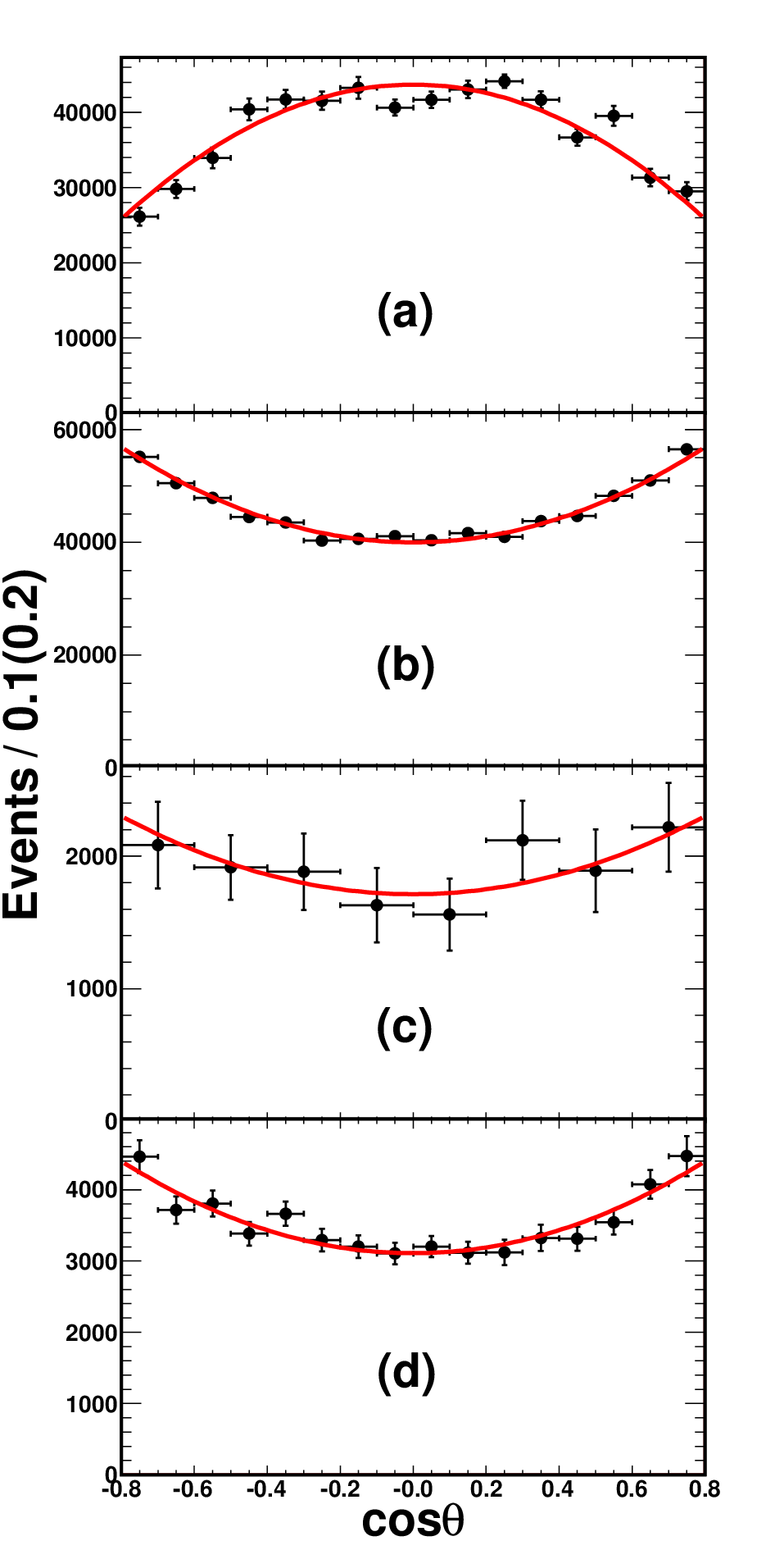
- 4.
The reconstruction efficiency, which includes the two photon efficiencies, reconstruction efficiency and the reconstruction efficiency, is studied with the control sample via single and double tag methods. The selection criteria of the charged tracks, and the reconstruction of and candidates are exactly same as those described in Sec. 3. The reconstruction efficiency is defined as the ratio of the number of events from the double tag to that from the single tag. The difference in the reconstruction efficiency between data and MC samples is taken as the systematic uncertainty.
- 5.
In the fits of the signal, the uncertainty due to the fitting range is estimated by varying the mass range by 10 MeV/ for two sides. The resulting differences of signal yields are taken as the systematic uncertainty.
- 6.
The uncertainties due to the background shape arise from the polynomial function and the peaking shape. The former is estimated by the alternative fits with a first or a third-order polynomial function. The latter is estimated by varying the number of normalized events by 1. The larger difference is taken as the systematic uncertainty. The total uncertainty related to the background shape is obtained by adding all contributions in quadrature.
- 7.
The systematic uncertainty due to the wrong combination background is estimated by comparing the signal yields between the fits with and without the corresponding component included in the fit. The differences of signal yields are taken as systematic uncertainties.
- 8.
The uncertainty related with the detection efficiency due to the modeling of the angular distribution of the baryon pairs, represented by the parameter , is estimated by varying the measured values by 1 in the MC simulation. The changes in the detection efficiency are taken as a systematic uncertainty.
- 9.
The systematic uncertainties due to the branching fractions of the intermediate states, , and , are taken from the PDG [4]. They are 1.9% for and 0.8% for .
- 10.
The various systematic uncertainties on the branching fraction measurements are summarized in Table 2. The total systematic uncertainty is obtained by summing the individual contributions in quadrature.
| Source | ||||
|---|---|---|---|---|
| Photon efficiency | 2.0 | … | 2.0 | … |
| reconstruction | 1.0 | … | 1.0 | … |
| reconstruction | 3.0 | … | 1.0 | … |
| reconstruction | … | 2.6 | … | 2.6 |
| Fit range | 2.1 | 1.6 | 2.8 | 1.8 |
| Background shape | 3.9 | 1.5 | 4.0 | 2.3 |
| Wrong combination | 4.2 | 0.8 | 4.5 | 0.3 |
| Angular distribution | 2.0 | 0.5 | 1.2 | 2.8 |
| Intermediate decay | 1.9 | 0.8 | 1.9 | 0.8 |
| Total number of | 0.5 | 0.5 | 0.6 | 0.6 |
| Total | 7.7 | 3.7 | 7.4 | 4.9 |
6.2 Angular distribution
Various systematic uncertainties are considered in the measurement of the values of . These include the uncertainty of the signal yield in the different intervals, the uncertainty of the fit procedure, and the uncertainty related to the detection efficiency correction curve as function of the bin. They are discussed in detail below.
- 1.
The signal yields in each interval are determined by the fit to the corresponding distribution. The sources of the systematic uncertainty of the signal yield include the fit range, the background shape, MC resolution and wrong combination, where the MC resolution is fixed for the decay only. To estimate the systematic uncertainty related with fit range on , we repeat the fit to the distribution by changing the fit range by 10 MeV/. Then, the values are extracted by the fit with the changed signal yield, and the resulting differences to the nominal values are taken as the systematic uncertainties. The uncertainties related to the background shape, MC resolution and wrong combination backgrounds in the fit are evaluated with a method similar to the one described above.
- 2.
The systematic uncertainties related to the procedure of the fit on the distribution are estimated by re-fitting the distribution with a different binning and fit range. We divide into 8 intervals for and 16 intervals for . The changes of the values are taken as systematic uncertainties. We also repeat the fit by changing the range to [0.9, 0.9] or [0.7, 0.7] in , with the same bin size of the nominal fit. The largest differences of value with respect to the nominal value are taken as a systematic uncertainties.
- 3.
In the analysis, the values are obtained by fitting the distribution corrected by the detection efficiency. To estimate the systematic uncertainty related to the imperfect simulation of the detection efficiency, the ratio of detection efficiencies as function of between data and MC simulation is obtained based on the control sample with a full event reconstruction. Then, the efficiency corrected distribution scaled by the ratios of detection efficiencies is refitted. The resulting differences in are taken as the systematic uncertainty.
All the systematic uncertainties for the measurement are summarized in Table 3. The total systematic uncertainty is the quadratic sum of the individual values.
| Source | ||||
|---|---|---|---|---|
| fitting range | 7.8 | 3.0 | 15.3 | 7.7 |
| Background shape | 3.2 | 3.0 | 20.0 | 4.6 |
| MC resolution | … | … | 16.9 | … |
| Wrong combination | 4.7 | 1.5 | 5.1 | 15.0 |
| interval | 7.8 | 3.5 | 22.0 | 10.4 |
| fitting range | 7.8 | 3.0 | 15.6 | 3.5 |
| Efficiency correction | 4.7 | 3.0 | 9.0 | 3.0 |
| Total | 15.4 | 7.1 | 41.8 | 20.8 |
7 Conclusion and discussion
Using and events collected with the BESIII detector at BEPCII, the branching fractions and the angular distributions for and are measured. A comparison of the branching fractions between our measurement and previous experiments (PDG average) is summarized in Table 4. The branching fractions for are measured for the first time, and the branching fractions for are measured with a good agreement and a much higher precision than the previous results. The measured values are also compared with the predictions of the theoretical models from Refs. [6, 7]. As indicated in Table 5, some of our results disagree significantly with the theoretical predictions, which may imply that the naive prediction of QCD suffers from the approximation that higher-order corrections are not taken into account. As calculated in Ref. [9], the sign for parameter in mode could be negative if re-scattering effects in the final states are taken into account. However, our results show that for is negative, and is different to the other decay processes in this measurement, which is hard to explain within the existing models. We, therefore, believe that it is of utmost importance to improve the theoretical models to shed further light on the origin of these discrepancies.
| Mode | ||||
| This work | ||||
| BESII [23] | … | … | … | |
| CLEO [24] | … | … | … | |
| Dobbs et al. [25] | … | … | … | |
| PDG [4] | … | … |
| Mode | ||||
|---|---|---|---|---|
| This work | 0.64 0.03 0.10 | 0.59 0.25 0.25 | ||
| Carimalo et al. [6] | 0.11 | 0.16 | 0.28 | 0.33 |
| Claudson [7] | 0.19 | 0.28 | 0.46 | 0.53 |
To test the “12% rule", the ratios of the branching fractions and are calculated to be (6.44 0.47 0.64)% and (23.43 0.26 1.09)%, respectively, taking into account the cancelation of the common systematic uncertainties. The ratios are not in agreement with 12%, especially for the final state.
To test isospin symmetry, the ratios of the branching fractions listed in Table 6 are also calculated based on the measurements between the neutral mode and the corresponding charged modes [13] taking into account the cancelation of the common systematic uncertainties. All ratios are within of the expectation of isospin symmetry.
| Mode | |||
|---|---|---|---|
8 Acknowledgement
The BESIII collaboration thanks the staff of BEPCII and the IHEP computing center for their strong support. This work is supported in part by National Key Basic Research Program of China under Contract No. 2015CB856700; National Natural Science Foundation of China (NSFC) under Contracts Nos. 11235011, 11322544, 11335008, 11425524, 11475207, 11505034, 11565006, 11635010; the Chinese Academy of Sciences (CAS) Large-Scale Scientific Facility Program; the CAS Center for Excellence in Particle Physics (CCEPP); the Collaborative Innovation Center for Particles and Interactions (CICPI); Joint Large-Scale Scientific Facility Funds of the NSFC and CAS under Contracts Nos. U1232107, U1232201, U1332201, U1532257, U1532258; CAS under Contracts Nos. KJCX2-YW-N29, KJCX2-YW-N45; 100 Talents Program of CAS; National 1000 Talents Program of China; INPAC and Shanghai Key Laboratory for Particle Physics and Cosmology; German Research Foundation DFG under Contracts Nos. Collaborative Research Center CRC 1044, FOR 2359; Istituto Nazionale di Fisica Nucleare, Italy; Koninklijke Nederlandse Akademie van Wetenschappen (KNAW) under Contract No. 530-4CDP03; Ministry of Development of Turkey under Contract No. DPT2006K-120470; The Swedish Resarch Council; U. S. Department of Energy under Contracts Nos. DE-FG02-05ER41374, DE-SC-0010504, DE-SC-0010118, DE-SC-0012069; U.S. National Science Foundation; University of Groningen (RuG) and the Helmholtzzentrum fuer Schwerionenforschung GmbH (GSI), Darmstadt; WCU Program of National Research Foundation of Korea under Contract No. R32-2008-000-10155-0.
9 References
References
- [1] S. J. Brodsky and G. P. Lepage, Phys. Rev. D 24 (1981) 2848; J. Bolz and P. Kroll, Eur. Phys. J. C 2 (1998) 545; R. G. Ping, H. C. Chiang and B. S. Zou, Phys. Rev. D 66 (2002) 054020.
- [2] T. Appelquist and H. D. Politzer, Phys. Rev. Lett. 34 (1975) 43; D. M. Asner et al., Int. J. Mod. Phys. A 24 (2009).
- [3] Y. F. Gu and X. H. Li, Phys. Rev. D 63 (2001) 114019; X. H. Mo, C. Z. Yuan and P. Wang, High Energy Physics and Nuclear Physics 31 (2007) 686 ; Quarkonium Working Group, N. Brambilla et al., Eur. Phys. J. C 71 (2011) 1534 ; Q. Wang, G. Li, and Q. Zhao, Phys. Rev. D 85 (2012) 074015.
- [4] Particle Data Group, C. Patrignani et al., Chin. Phys. C 40 (2016) 100001.
- [5] F. Murgia and M. Melis, Phys. Rev. D 51 (1995) 3487; BES Collaboration, J. Z. Bai, et al., Phys. Lett. B 591 (2004) 42; BES Collaboration, M. Ablikim, et al., Phys. Lett. B 632 (2006) 181; Fermilab E835 Collaboration, A. Buzzo, et al., Phys. Lett. B 610 (2005) 177.
- [6] C. Carimalo, Int. J. Mod. Phys. A 2 (1987) 249.
- [7] M. Claudson, S. L. Glashow and M. B. Wise, Phys. Rev. D 25(1982) 1345.
- [8] BES Collaboration, M. Ablikim et al., Phys. Lett. B 632 (2006) 181.
- [9] H. Chen and R. G. Ping, Phys. Lett. B 644 (2007) 54.
- [10] BES Collaboration, J. Z. Bai et al., Phys. Lett. B 591 (2004).
- [11] BES Collaboration, M. Ablikim et al., Phys. Lett. B 648 (2007) 149.
- [12] BES Collaboration, M. Ablikim et al., Chin. Phys. C 36 (2012) 1031.
- [13] BESIII Collaboration, M. Ablikim et al., Phys. Rev. D 93 (2016) 072003.
- [14] BESIII Collaboration, M. Ablikim et al., Chin. Phys. C 41 (2017) no.1, 013001.
- [15] BESIII Collaboration, M. Ablikim et al., Chin. Phys. C 37 (2013) 063001.
- [16] With the same method (see Ref. [15] for more details), the preliminary number of the events taken in 2009 and 2012 determined to be with an uncertainty of 0.6%.
- [17] BESIII Collaboration, M. Ablikim et al., Nucl. Instrum. Meth. A 614 (2010) 345.
- [18] GEANT4 Collaboration, S. Agostinelli et al., Nucl. Instrum. Meth. A 506 (2003) 250; J. Allison et al., IEEE Trans. Nucl. Sci. 53 (2006) 270 .
- [19] S. Jadach, B. F. L. Ward and Z. Was, Comput. Phys. Commun. 130 (2000) 260; S. Jadach, B. F. L. Ward and Z. Was, Phys. Rev. D 63 (2001) 113009.
- [20] R. G. Ping et al., Chin. Phys. C 32 (2008) 599; D. J. Lange, Nucl. Instrum. Meth. A 462 (2001) 152.
- [21] J. C. Chen, G. S. Huang, X. R. Qi, D. H. Zhang and Y. S. Zhu, Phys. Rev. D 62 (2000) 034003.
- [22] BESIII Collaboration, M. Ablikim, et al., Phys. Rev. D 87 (3) (2013) 032007.
- [23] BES Collaboration, M. Ablikim et al., Phys. Rev. D 78 (2008) 092005.
- [24] CLEO Collaboration, T. K. Pedlar et al., Phys. Rev. D 72 (2005) 051108.
- [25] S. Dobbs, A. Tomaradze, T. Xiao, K. K. Seth and G. Bonvicini, Phys. Lett. B 739 (2014) 90.