跳到论文正文
W Papers独立论文阅读器 arXiv:1612.08576 论文正文 计算阅读时间 · 0%
引用这篇论文根据当前论文元数据生成,正式投稿前建议核对。


License: arXiv.org perpetual non-exclusive license
arXiv:1612.08576v1 [hep-ph] 27 Dec 2016

A STUDY OF STRUCTURE FUNCTIONS WITH THE DGLAP EQUATIONS AT SMALL xx WITH O⁡(x)O(x) AND O⁡(x2)O(x^{2}) .

Luxmi Machahari Affiliation: Department of Physics, Gauhati University, Guwahati-781 014, India. Affiliation: email:luxmimachahari@gmail.com    D. K. Choudhury Affiliation: Department of Physics, Gauhati University, Guwahati-781 014, India. Affiliation: Physics Academy of North-East, Guwahati-781 014, India. Affiliation: email:dkc_\_phys@yahoo.co.in    P.K.Sahariah Affiliation: Department of Physics,Cotton College,Guwahati 781001, India Affiliation: email:pksahariah@gmail.com
Abstract

We obtain a pair of second order differential equations in two variables xx and tt from the coupled DGLAP QCD evolution equations at small xx using the standard Taylor series expansion method.To that end we keep terms upto O⁡(x2)O(x^{2}).We use the standard assumption about the relationship between the singlet Structure Function and the gluon distributions available in current literature. We solve the taylor approximated O⁡(x)O(x) DGLAP equations by Lagranges auxiliary method and O⁡(x2)O(x^{2}) equation by Method of Separation of Variables and then show that the two solutions obtained in each for O⁡(x)O(x) and O⁡(x2)O(x^{2}) are not identical in general.Analysis of the results obtained are done in the range of the recent HERA data.

1 Introduction

The parton distribution function of the nucleon is an essential ingredient in any high energy physics experiments.The distribution functions which are functions of the Bjorken variable xx and the four momentum tranfer squared Q2Q^{2} between the lepton and the hadron in DIS experiment, is not calculable in theory but its evolution in Q2Q^{2} can be predicted by perturbative QCD method. The DGLAP equations [1, 2, 3, 4, 5] are the essential tools to calculate the evolution of the parton distributions and the structure functions of the nucleon and nuclei. These equations are integro-differential equations whose complexity rises as we move to higher and higher order. These equations are normally solved numerically taking into account the world data on lepton hadron scattering [6]. But alternatively the evolution equations can also be solved analytically under certain assumptions valid to be at low xx [7, 9, 8, 12]. In reference [7, 9, 8, 12] several authors make a Taylor approximation and convert the integro differential DGLAP equations into first order partial differential equations in both xx and tt where xx is Bjorken variable and t=t=log(Q2Λ2)(\frac{Q^{2}}{\Lambda^{2}}) and Λ\Lambda as QCD scale parameter.As a second step, an ansatz relating gluon and singlet structure Function is assumed [8] to make them analytically solvable. In the present paper we rederive the solutions of the coupled DGLAP equations of O⁡(x)O(x) in LO at low xx and show that with such an ansatz the two equations in the coupled set lead to two different non-unique solutions by Lagranges Auxiliary method, a feature overlooked in Ref[7, 9, 8, 12].Similarly we derive the solutions of the coupled DGLAP equations of O⁡(x2)O(x^{2}) in LO at low xx by a very basic method of Separation of Variables and using the same ansatz, the coupled set lead to again two non-unique solutions.

In sections 2, we outline a brief formalism,section 3 shows the results and the conclusions are highlighted in section 4. This paper reports a set of Taylor approximated O⁡(x)O(x) and O⁡(x2)O(x^{2}) DGLAP Ref.[1, 2, 3, 4] equations at small xx using the Lagranges method and the Method of seperation of Variables respectively .

2 Formalism

The coupled DGLAP equations for quark and gluon parton distribution function defined as q⁡(x,t)q(\textit{x},\textit{t}) and g⁡(x,t)g(\textit{x},\textit{t}) at leading order (LO) are given in Ref.[5]

t​∂∂t​qi​(x,t)=αs​(t)2​π​∑qi​q¯i∫x1d​zz​[CF​{(1+z2)(1−z)++32​δ​(1−z)}​qi​(xz,t)+TR​{z2+(1−z)2}​g​(xz,t)]t\frac{\partial}{\partial t}q_{i}(x,t)=\frac{\alpha_{s}(t)}{2\pi}\sum_{q_{i}\overline{q}_{i}}\int_{x}^{1}\dfrac{dz}{z}[C_{F}\left\{\frac{(1+z^{2})}{(1-z)_{+}}+\frac{3}{2}\delta(1-z)\right\}q_{i}(\frac{x}{z},t)+T_{R}\left\{z^{2}+(1-z)^{2}\right\}g(\frac{x}{z},t)] (1)
t∂∂tg(x,t)=αs​(t)2​π∑qi​q¯i∫x1d​zz[CF{1+(1−z)2z}qi(xz,t)+{2CA(z(1−z)+1−zz+z(1−z))+δ(1−z)11​CA−4​Nf​TR6}g(xz,t)],t\frac{\partial}{\partial t}g(x,t)=\frac{\alpha_{s}(t)}{2\pi}\sum_{q_{i}\overline{q}_{i}}\int_{x}^{1}\frac{dz}{z}[C_{F}\left\{\frac{1+(1-z)^{2}}{z}\right\}q_{i}(\frac{x}{z},t)+\{2C_{A}\left(\frac{z}{(1-z)_{+}}\frac{1-z}{z}+z(1-z)\right)\\ +\delta(1-z)\frac{11C_{A}-4N_{f}T_{R}}{6}\}g(\frac{x}{z},t)], (2)

where, i is any quark flavor , t=log⁡(Q2Λ2)t=\log(\frac{Q^{2}}{\Lambda^{2}}) , Q2Q^{2} is four momentum transfer squared with Λ\Lambda as QCD scale parameter. αs\alpha_{s} is the strong coupling constant which is given in LO by αs​(Q2)=12​π(33−2​Nf)​l​o​g​(Q2/Λ2)\alpha_{s}(Q^{2})=\frac{12\pi}{(33-2N_{f})log(Q^{2}/\Lambda^{2})}
The other constants are TR=12,CA=3,CF=43T_{R}=\frac{1}{2},\ \ \ C_{A}=3,\ \ \ C_{F}=\frac{4}{3} and NfN_{f} is the number of quark Flavours.
The subindex ′+′{}^{\prime}+^{\prime} in the term 1(1−z)+\frac{1}{(1-z)_{+}} is a plus distribution which indicates the cancellation of the divergence that is appearing at z=1z=1 through

∫01d​z​f⁡(z)(1−z)+=∫01d​z​f⁡(z)−f⁡(1)1−z\int_{0}^{1}dz\frac{f(z)}{(1-z)_{+}}=\int_{0}^{1}dz\frac{f(z)-f(1)}{1-z}

where, f⁡(z)f(z) is any arbitrary function.
We reduce this integrodifferential equation to a calculable partial differential equation by defining a new variable u=1−zu=1-z and expanding 1z\frac{1}{z} as[9]

1z=1u=∑r=0∞ur=1+∑r=1∞ur\frac{1}{z}=\frac{1}{u}=\sum_{r=0}^{\infty}u^{r}=1+\sum_{r=1}^{\infty}u^{r} (3)

Using the Taylor series upto the second order O(x2)(\textit{x}^{2}) for small x for quarks and gluon distributions qi​(xz)q_{i}(\frac{x}{z}) and g⁡(xz)g(\frac{x}{z}) can be written respectively as

qi​(xz,t)=qi​(x,t)+x​∑r=1∞ur​∂∂x​qi​(x,t)+x22!​(∑r=1∞ur)2​∂2∂x2​qi​(x,t)q_{i}(\frac{x}{z},t)=q_{i}(x,t)+x\sum_{r=1}^{\infty}u^{r}\frac{\partial}{\partial x}q_{i}(x,t)+\frac{x^{2}}{2!}(\sum_{r=1}^{\infty}u^{r})^{2}\frac{\partial^{2}}{\partial x^{2}}q_{i}(x,t) (4)
g⁡(xz,t)=g⁡(x,t)+x​∑r=1∞ur​∂∂x​g​(x,t)+x22!​(∑r=1∞ur)2​∂2∂x2​g​(x,t)g(\frac{x}{z},t)=g(x,t)+x\sum_{r=1}^{\infty}u^{r}\frac{\partial}{\partial x}g(x,t)+\frac{x^{2}}{2!}(\sum_{r=1}^{\infty}u^{r})^{2}\frac{\partial^{2}}{\partial x^{2}}g(x,t) (5)

Using equations (4)and (5) in eqn.(1) the Taylor approximated form of the coupled DGLAP equations are:

t∂∂tqi(x,t)=αs​(t)2​π∑qi​q¯i∫x1d​zz[CF{(1+z2)(1−z)++32δ(1−z)}{qi(x,t)+x∑r=1∞ur∂∂xqi(x,t)+x22!(∑r=1∞ur)2∂2∂x2qi(x,t)}+TR{z2+(1−z)2}{g(x,t)+x∑r=1∞ur∂∂xg(x,t)+x22!(∑r=1∞ur)2∂2∂x2g(x,t)}]t\frac{\partial}{\partial t}q_{i}(x,t)=\frac{\alpha_{s}(t)}{2\pi}\sum_{q_{i}\overline{q}_{i}}\int_{x}^{1}\dfrac{dz}{z}[C_{F}\left\{\frac{(1+z^{2})}{(1-z)_{+}}+\frac{3}{2}\delta(1-z)\right\}\{q_{i}(x,t)+x\sum_{r=1}^{\infty}u^{r}\frac{\partial}{\partial x}q_{i}(x,t)\\ +\frac{x^{2}}{2!}(\sum_{r=1}^{\infty}u^{r})^{2}\frac{\partial^{2}}{\partial x^{2}}q_{i}(x,t)\}+T_{R}\left\{z^{2}+(1-z)^{2}\right\}\{g(x,t)+x\sum_{r=1}^{\infty}u^{r}\frac{\partial}{\partial x}g(x,t)\\ +\frac{x^{2}}{2!}(\sum_{r=1}^{\infty}u^{r})^{2}\frac{\partial^{2}}{\partial x^{2}}g(x,t)\}] (6)

Similarly equation(2) can be written as

t∂∂tg(x,t)=αs​(t)2​π∑qi​q¯i∫x1d​zz[CF{1+(1−z)2z}{qi(x,t)+x∑r=1∞ur∂∂xqi(x,t)+x22!(∑r=1∞ur)2∂2∂x2qi(x,t)}+{2CA(z(1−z)++1−zz+z(1−z))+δ(1−z)11​CA−4​Nf​TR6}{g(x,t)+x∑r=1∞ur∂∂xg(x,t)+x22!(∑r=1∞ur)2∂2∂x2g(x,t)}]t\frac{\partial}{\partial t}g(x,t)=\frac{\alpha_{s}(t)}{2\pi}\sum_{q_{i}\overline{q}_{i}}\int_{x}^{1}\frac{dz}{z}[C_{F}\left\{\frac{1+(1-z)^{2}}{z}\right\}\{q_{i}(x,t)+x\sum_{r=1}^{\infty}u^{r}\frac{\partial}{\partial x}q_{i}(x,t)+\frac{x^{2}}{2!}(\sum_{r=1}^{\infty}u^{r})^{2}\frac{\partial^{2}}{\partial x^{2}}q_{i}(x,t)\}\\ +\{2C_{A}\left(\frac{z}{(1-z)_{+}}+\frac{1-z}{z}+z(1-z)\right)+\delta(1-z)\frac{11C_{A}-4N_{f}T_{R}}{6}\}\{g(x,t)\\ +x\sum_{r=1}^{\infty}u^{r}\frac{\partial}{\partial x}g(x,t)+\frac{x^{2}}{2!}(\sum_{r=1}^{\infty}u^{r})^{2}\frac{\partial^{2}}{\partial x^{2}}g(x,t)\}] (7)

Equations (6) and (7) can be written in compact form as:

t​∂∂t​qi​(x,t)=αs​(t)2​π​∑qi​q¯i[{J1​(x)+x​J2​(x)​∂∂x+x2​J3​(x)​∂2∂x2}​qi​(x,t)+{J4​(x)+x​J5​(x)​∂∂x+x2​J6​(x)​∂2∂x2}​g​(x,t)]t\frac{\partial}{\partial t}q_{i}(x,t)=\frac{\alpha_{s}(t)}{2\pi}\sum_{q_{i}\overline{q}_{i}}[\{J_{1}(x)+xJ_{2}(x)\frac{\partial}{\partial x}+x^{2}J_{3}(x)\frac{\partial^{2}}{\partial x^{2}}\}q_{i}(x,t)+\{J_{4}(x)+xJ_{5}(x)\frac{\partial}{\partial x}+x^{2}J_{6}(x)\frac{\partial^{2}}{\partial x^{2}}\}g(x,t)] (8)
t​∂∂t​g​(x,t)=αs​(t)2​π​∑qi​q¯i[{J7​(x)+x​J8​(x)​∂∂x+x2​J9​(x)​∂2∂x2}​qi​(x,t)+{J10​(x)+x​J11​(x)​∂∂x+x2​J12​(x)​∂2∂x2}​g​(x,t)]t\frac{\partial}{\partial t}g(x,t)=\frac{\alpha_{s}(t)}{2\pi}\sum_{q_{i}\overline{q}_{i}}[\{J_{7}(x)+xJ_{8}(x)\frac{\partial}{\partial x}+x^{2}J_{9}(x)\frac{\partial^{2}}{\partial x^{2}}\}q_{i}(x,t)+\{J_{10}(x)+xJ_{11}(x)\frac{\partial}{\partial x}+x^{2}J_{12}(x)\frac{\partial^{2}}{\partial x^{2}}\}g(x,t)] (9)

The expressions for J1,J2,J3,…​…..J12J_{1},J_{2},J_{3},........J_{12} are as given in the Appendix A.
Neglecting the O⁡(x2)O(x^{2}) terms in the equations (8) and (9), the corresponding DGLAP equations in O⁡(x)O(x) are as follows

t​∂∂t​qi​(x,t)=αs​(t)2​π​∑qi​q¯i[{J1​(x)+x​J2​(x)​∂∂x}​qi​(x,t)+{J4​(x)+x​J5​(x)​∂∂x}​g​(x,t)]t\frac{\partial}{\partial t}q_{i}(x,t)=\frac{\alpha_{s}(t)}{2\pi}\sum_{q_{i}\overline{q}_{i}}[\{J_{1}(x)+xJ_{2}(x)\frac{\partial}{\partial x}\}q_{i}(x,t)+\{J_{4}(x)+xJ_{5}(x)\frac{\partial}{\partial x}\}g(x,t)] (10)
t​∂∂t​g​(x,t)=αs​(t)2​π​∑qi​q¯i[{J7​(x)+x​J8​(x)​∂∂x}​qi​(x,t)+{J10​(x)+x​J11​(x)​∂∂x}​g​(x,t)]t\frac{\partial}{\partial t}g(x,t)=\frac{\alpha_{s}(t)}{2\pi}\sum_{q_{i}\overline{q}_{i}}[\{J_{7}(x)+xJ_{8}(x)\frac{\partial}{\partial x}\}q_{i}(x,t)+\{J_{10}(x)+xJ_{11}(x)\frac{\partial}{\partial x}\}g(x,t)] (11)

To obtain the qualitative feature of our work, at the quark level,for a single quark flavor, we use the relation:

g⁡(x,t)=C⁡(t)​q​(x,t)g(x,t)=C(t)q(x,t) (12)

Where, C⁡(t)C(t) is an xx independent and tt dependent function compatible with the analysis of Lopez and Yndurain [14]. Using eqn.(12) in equations(8) and (9) and also in equations(10) and (11) and we obtain the following pair of 1s​t1^{st} and 2n​d2^{nd} order differential equations respectively as follows:

t​∂∂t​q​(x,t)=αs​(t)2​π​[J1​(x)+J4​(x)​C​(t)]​q​(x,t)+αs​(t)2​π​x​[J2​(x)+J5​(x)​C​(t)]​∂∂x​q​(x,t)t\frac{\partial}{\partial t}q(x,t)=\frac{\alpha_{s}(t)}{2\pi}[J_{1}(x)+J_{4}(x)C(t)]q(x,t)+\frac{\alpha_{s}(t)}{2\pi}x[J_{2}(x)+J_{5}(x)C(t)]\frac{\partial}{\partial x}q(x,t) (13)
t​∂∂t​(C⁡(t)​q​(x,t))=αs​(t)2​π​[J7​(x)+J10​(x)​C​(t)]​q​(x,t)+αs​(t)2​π​x​[J8​(x)+J11​(x)​C​(t)]​∂∂x​q​(x,t)t\frac{\partial}{\partial t}(C(t)q(x,t))=\frac{\alpha_{s}(t)}{2\pi}[J_{7}(x)+J_{10}(x)C(t)]q(x,t)+\frac{\alpha_{s}(t)}{2\pi}x[J_{8}(x)+J_{11}(x)C(t)]\frac{\partial}{\partial x}q(x,t) (14)

and

t∂∂tq(x,t)=αs​(t)2​π[J1(x)+J4(x)C(t)]q(x,t)+αs​(t)2​πx[J2(x)+J5(x)C(t)]∂∂xq(x,t)+αs​(t)2​πx2[J3(x)+J6(x)C(t)]∂2∂x2q(x,t)t\frac{\partial}{\partial t}q(x,t)=\frac{\alpha_{s}(t)}{2\pi}[J_{1}(x)+J_{4}(x)C(t)]q(x,t)+\frac{\alpha_{s}(t)}{2\pi}x[J_{2}(x)+J_{5}(x)C(t)]\frac{\partial}{\partial x}q(x,t)+\frac{\alpha_{s}(t)}{2\pi}x^{2}[J_{3}(x)\\ +J_{6}(x)C(t)]\frac{\partial^{2}}{\partial x^{2}}q(x,t) (15)
t​∂∂t​(C⁡(t)​q​(x,t))=αs​(t)2​π​[J7​(x)+J10​(x)​C​(t)]​q​(x,t)+αs​(t)2​π​x​[J8​(x)+J11​(x)​C​(t)]​∂∂x​q​(x,t)+αs​(t)2​π​x2​[J9​(x)+J12​(x)​C​(t)]​∂2∂x2​q​(x,t)t\frac{\partial}{\partial t}(C(t)q(x,t))=\frac{\alpha_{s}(t)}{2\pi}[J_{7}(x)+J_{10}(x)C(t)]q(x,t)+\frac{\alpha_{s}(t)}{2\pi}x[J_{8}(x)+J_{11}(x)C(t)]\frac{\partial}{\partial x}q(x,t)\\ +\frac{\alpha_{s}(t)}{2\pi}x^{2}[J_{9}(x)+J_{12}(x)C(t)]\frac{\partial^{2}}{\partial x^{2}}q(x,t) (16)

equations (15) and (16) are solved by using the standard Lagranges Method [10].To apply Lagrange’s Method, we put the two above equations (13) and (14) in the form as

Q1​(x,t)​∂∂t​q​(x,t)+P1​(x,t)​∂∂x​q​(x,t)=R1​(x,t)Q_{1}(x,t)\frac{\partial}{\partial t}q(x,t)+P_{1}(x,t)\frac{\partial}{\partial x}q(x,t)=R_{1}(x,t) (17)
Q2​(x,t)​∂∂t​q​(x,t)+P2​(x,t)​∂∂x​q​(x,t)=R2​(x,t)Q_{2}(x,t)\frac{\partial}{\partial t}q(x,t)+P_{2}(x,t)\frac{\partial}{\partial x}q(x,t)=R_{2}(x,t) (18)

Where, Q1​(x,t),P1​(x,t),R1​(x,t),Q2​(x,t),P2​(x,t),R2​(x,t)Q_{1}(x,t),P_{1}(x,t),R_{1}(x,t),Q_{2}(x,t),P_{2}(x,t),R_{2}(x,t) are obtained by comparing equation(17) with equation(13) and equation(18) with equation(14) given in Appendix B.

The general solution of equation (17) and (18) is obtained by solving the following auxillary system of ordinary differential equations.

d​xPm​(x,t)=d​tQm​(x,t)=d​q​(x,t)Rm​(x,t)\frac{dx}{P_{m}(x,t)}=\frac{dt}{Q_{m}(x,t)}=\frac{dq(x,t)}{R_{m}(x,t)} (19)

Where, m goes from 1 to 2 referring respectively the two equations (17) and (18) and
If um​(x,t,q⁡(x,t))=Cmu_{m}(x,t,q(x,t))=C_{m} and vm​(x,t,q⁡(x,t))=Dmv_{m}(x,t,q(x,t))=D_{m} are two independent solutions of the above equations (17) and (18),then in general their solutions are

fm​(um,vm)=0f_{m}(u_{m},v_{m})=0 (20)

where, fmf_{m} are arbitrary functions of umu_{m} and vmv_{m}.
Solving the auxillary equations, we get

u1​(x,t,q⁡(x,t))=t​X1​(x,t)\displaystyle u_{1}(x,t,q(x,t))=tX_{1}(x,t) (21)
v1​(x,t,q⁡(x,t))=q⁡(x,t)​Y1​(x,t)\displaystyle v_{1}(x,t,q(x,t))=q(x,t)Y_{1}(x,t) (22)

And,

u2​(x,t,q⁡(x,t))=X2​(x,t)\displaystyle u_{2}(x,t,q(x,t))=X_{2}(x,t) (23)
v2​(x,t,q⁡(x,t))=q⁡(x,t)​Y2​(x,t)\displaystyle v_{2}(x,t,q(x,t))=q(x,t)Y_{2}(x,t) (24)

Where X1​(x,t),X2​(x,t),Y1​(x,t),Y2​(x,t)X_{1}(x,t),X_{2}(x,t),Y_{1}(x,t),Y_{2}(x,t) are in Appendix B. The simplest possibility of finding a unique expression for q⁡(x,t)q(x,t) to satisfy the general solution (20) is the linear combination of umu_{m} and vmv_{m} in q⁡(x,t)q(x,t) such as,

um+αm​vm=βmu_{m}+\alpha_{m}v_{m}=\beta_{m} (25)

Where, αm\alpha_{m} and βm\beta_{m} are the quantities to be determined from boundary conditions on q⁡(x,t)q(x,t). Considering m=1m=1 and putting the expressions for u1u_{1} and v1v_{1} as in equations (21) and (22) in the above equation(25) we get the corresponding solution as

qI​(x,t)=1α1​[β1Y1​(x,t)−t​X1​(x,t)Y1​(x,t)]q^{I}(x,t)=\frac{1}{\alpha_{1}}\left[\frac{\beta_{1}}{Y_{1}(x,t)}-t\frac{X_{1}(x,t)}{Y_{1}(x,t)}\right] (26)

Similarly for m=2 we obtain

qI​I​(x,t)=1α2​[β2Y2​(x,t)−X2​(x,t)Y2​(x,t)]q^{II}(x,t)=\frac{1}{\alpha_{2}}\left[\frac{\beta_{2}}{Y_{2}(x,t)}-\frac{X_{2}(x,t)}{Y_{2}(x,t)}\right] (27)

where α1,α2,β1\alpha_{1},\alpha_{2},\beta_{1} and β2\beta_{2} are four unknown parameters.The algebraic structures show that (26)≠\neq(27).

To obtain a corresponding information for second order we use the method of Separation of Variables [11] instead,which means all Parton Distribution Functions are factorizable in xx and tt.Under this assumption we can write

qI​(x,t)=X⁡(x)​T​(t)q^{I}(x,t)=X(x)T(t) (28)
qI​I​(x,t)=X^​(x)​T^​(t)q^{II}(x,t)=\hat{X}(x)\hat{T}(t) (29)

To go further we have to put some information of C⁡(t)C(t).Assuming C⁡(t)=kC(t)=k(constant) [8],We obtain the solutions for T⁡(t)T(t) and T^​(t)\hat{T}(t) as

T⁡(t)=exp⁡[−s2​631​(1t−1t0)]T(t)=\exp[-s^{2}\frac{6}{31}(\frac{1}{t}-\frac{1}{t_{0}})] (30)

and

T^​(t)=exp⁡[−s^2​631​k​(1t−1t0)]\hat{T}(t)=\exp[-\hat{s}^{2}\frac{6}{31k}(\frac{1}{t}-\frac{1}{t_{0}})] (31)

where s2s^{2} and s^2\hat{s}^{2} are positive separation constants and for any initial scale at Q2=Q02Q^{2}=Q_{0}^{2} , t0=l​o​g​(Q02Λ2)t_{0}=log(\frac{Q_{0}^{2}}{\Lambda^{2}}).In obtaining both the expressions we used at any initial scale at Q2=Q02Q^{2}=Q_{0}^{2} (i.e at t=t0t=t_{0}),the input distribution is a function of xx only.Hence q⁡(x,t0)=X⁡(x)q(x,t_{0})=X(x) or X^​(x)\hat{X}(x) and so T⁡(t0)=T^​(t0)=1T(t_{0})=\hat{T}(t_{0})=1. Depending on the nature of equations Hyperbolic,Parabolic and Elliptic [10].X⁡(x)X(x) has three solutions:
a) X⁡(x)=[c1​em1.x+c2​em2.x]X(x)=\left[c_{1}e^{m_{1}.x}+c_{2}e^{m_{2}.x}\right], Hyperbolic
b) X⁡(x)=[c1​em.x+c2​x​em.x]X(x)=\left[c_{1}e^{m.x}+c_{2}xe^{m.x}\right], Parabolic
c) X⁡(x)=[eα​x​(c1​cos⁡β​x+c2​sin⁡β​x)]X(x)=\left[e^{\alpha x}(c_{1}\cos\beta x+c_{2}\sin\beta x)\right], Elliptic

Consequently qI​(x,t)q^{I}(x,t) have the following forms

qI​(x,t)=exp⁡[−s2​631​(1t−1t0)].[c1​em1.x+c2​em2.x]q^{I}(x,t)=\exp[-s^{2}\frac{6}{31}(\frac{1}{t}-\frac{1}{t_{0}})].\left[c_{1}e^{m_{1}.x}+c_{2}e^{m_{2}.x}\right] (32)
qI​(x,t)=exp⁡[−s2​631​(1t−1t0)].[c1​em.x+c2​x​em.x]q^{I}(x,t)=\exp[-s^{2}\frac{6}{31}(\frac{1}{t}-\frac{1}{t_{0}})].\left[c_{1}e^{m.x}+c_{2}xe^{m.x}\right] (33)
qI​(x,t)=exp⁡[−s2​631​(1t−1t0)].[eα​x​(c1​cos⁡β​x+c2​sin⁡β​x)]q^{I}(x,t)=\exp[-s^{2}\frac{6}{31}(\frac{1}{t}-\frac{1}{t_{0}})].\left[e^{\alpha x}(c_{1}\cos\beta x+c_{2}\sin\beta x)\right] (34)

and qI​I​(x,t)q^{II}(x,t) have the forms

qI​I​(x,t)=exp⁡[−s^2​631​k​(1t−1t0)].[c^1​e−B^+B^2−4​A^​C^2​A^.x+c^2​e−B^−B^2−4​A^​C^2​A^.x]q^{II}(x,t)=\exp[-\hat{s}^{2}\frac{6}{31k}(\frac{1}{t}-\frac{1}{t_{0}})].\left[\hat{c}_{1}e^{\frac{-\hat{B}+\sqrt{\hat{B}^{2}-4\hat{A}\hat{C}}}{2\hat{A}}.x}+\hat{c}_{2}e^{\frac{-\hat{B}-\sqrt{\hat{B}^{2}-4\hat{A}\hat{C}}}{2\hat{A}}.x}\right] (35)
qI​I​(x,t)=exp⁡[−s^2​631​k​(1t−1t0)].[c^1​em.x+c^2​x​em.x]q^{II}(x,t)=\exp[-\hat{s}^{2}\frac{6}{31k}(\frac{1}{t}-\frac{1}{t_{0}})].\left[\hat{c}_{1}e^{m.x}+\hat{c}_{2}xe^{m.x}\right] (36)
qI​I​(x,t)=exp⁡[−s^2​631​k​(1t−1t0)].[eα^​x​(c^1​cos⁡β^​x+c^2​sin⁡β^​x)]q^{II}(x,t)=\exp[-\hat{s}^{2}\frac{6}{31k}(\frac{1}{t}-\frac{1}{t_{0}})].\left[e^{\hat{\alpha}x}(\hat{c}_{1}\cos\hat{\beta}x+\hat{c}_{2}\sin\hat{\beta}x)\right] (37)

c1c_{1}, c2c_{2},c^1\hat{c}_{1}, and c^2\hat{c}_{2} are arbitrary constants. m1m_{1} and m2m_{2} are defined as m1=−B+B2−4.A.H2.A;m2=−B−B2−4.A.H2.A\ m_{1}=\frac{-B+\sqrt{B^{2}-4.A.H}}{2.A};\ \ m_{2}=\frac{-B-\sqrt{B^{2}-4.A.H}}{2.A} with

A⁡(x)=x2​[J3​(x)+J6​(x)​k]\displaystyle A(x)=x^{2}[J_{3}(x)+J_{6}(x)k]
B⁡(x)=x⁡[J2​(x)+J5​(x)​k]\displaystyle B(x)=x[J_{2}(x)+J_{5}(x)k]
H⁡(x)=[J1​(x)+J4​(x)​k]−s2\displaystyle H(x)=[J_{1}(x)+J_{4}(x)k]-s^{2} (38)

and

A^​(x)=x2​[J9​(x)+J12​(x)​k]\displaystyle\hat{A}(x)=x^{2}[J_{9}(x)+J_{12}(x)k]
B^​(x)=x⁡[J8​(x)+J11​(x)​k]\displaystyle\hat{B}(x)=x[J_{8}(x)+J_{11}(x)k]
H^​(x)=[J7​(x)+J12​(x)​k]−s^2\displaystyle\hat{H}(x)=[J_{7}(x)+J_{12}(x)k]-\hat{s}^{2} (39)

To obtain the above forms (32),(33),(34),(35),(36),(37) analytically we make further assumption besides method of Separation of Variables such as A⁡(x)≃A,B⁡(x,t)≃B,H⁡(x,t)≃HA(x)\simeq A,\ B(x,t)\simeq B,\ H(x,t)\simeq H which means that A,B,HA,B,H has a slow xx dependence.Thus here too from independent algebraic structures (32)≠(35),(33)≠(36),(34)≠(37)(\ref{E29})\neq(\ref{E32}),(\ref{E30})\neq(\ref{E33}),(\ref{E31})\neq(\ref{E34}). An observation of above equations shows that algebraic structures of qI​(x,t)q^{I}(x,t) and qI​I​(x,t)q^{II}(x,t) for each are different i.e qI​(x,t)≠qI​I​(x,t)q^{I}(x,t)\neq q^{II}(x,t).
To conclude, we obtain two inequivalent quark distribution for small xx DGLAP equations taking both the O⁡(x)O(x) and O⁡(x2)O(x^{2}) terms.

3 Results

In this section we show our results of O⁡(x)O(x) and O⁡(x2)O(x^{2}) graphically.

3.1 For O⁡(x)O(x):

We can write from equations (26) and (27)

qI​(x,t)=a1​(x,k)​[β1−t​ea2​(x,t,k)]q^{I}(x,t)=a_{1}(x,k)[\beta_{1}-te^{a_{2}(x,t,k)}] (40)
qI​I​(x,t)=a3​(x,k)​[β2−t​ea4​(x,t,k)]q^{II}(x,t)=a_{3}(x,k)[\beta_{2}-te^{a_{4}(x,t,k)}] (41)

where a1​(x,k),a2​(x,t,k),a3​(x,k),a4​(x,t,k)a_{1}(x,k),a_{2}(x,t,k),a_{3}(x,k),a_{4}(x,t,k) are given in Appendix C.
For the initial scale t=t0t=t_{0}

qI​(x,t0)=a1​(x,k)​[β1−t0​ea2​(x,t0,k)]q^{I}(x,t_{0})=a_{1}(x,k)[\beta_{1}-t_{0}e^{a_{2}(x,t_{0},k)}] (42)
qI​I​(x,t0)=a3​(x,k)​[β2−t0​ea4​(x,t0,k)]q^{II}(x,t_{0})=a_{3}(x,k)[\beta_{2}-t_{0}e^{a_{4}(x,t_{0},k)}] (43)

Now we take the ratio of eqn.(40) and (42) as

qI​(x,t)qI​(x,t0)=[β1−t​ea2​(x,t,k)][β1−t0​ea2​(x,t0,k)]\frac{q^{I}(x,t)}{q^{I}(x,t_{0})}=\frac{[\beta_{1}-te^{a_{2}(x,t,k)}]}{[\beta_{1}-t_{0}e^{a_{2}(x,t_{0},k)}]} (44)

ratio of eqn.(41) and (43)

qI​I​(x,t)qI​I​(x,t0)=[β2−t​ea4​(x,t,k)][β2−t0​ea4​(x,t0,k)]\frac{q^{II}(x,t)}{q^{II}(x,t_{0})}=\frac{[\beta_{2}-te^{a_{4}(x,t,k)}]}{[\beta_{2}-t_{0}e^{a_{4}(x,t_{0},k)}]} (45)

So,

qI​(x,t)=qI​(x,t0)​qI​(x,t)qI​(x,t0)q^{I}(x,t)=q^{I}(x,t_{0})\frac{q^{I}(x,t)}{q^{I}(x,t_{0})}
⟹qI​(x,t)=q⁡(x,t0)​[β1−t​ea2​(x,t,k)][β1−t0​ea2​(x,t0,k)]\implies q^{I}(x,t)=q(x,t_{0})\frac{[\beta_{1}-te^{a_{2}(x,t,k)}]}{[\beta_{1}-t_{0}e^{a_{2}(x,t_{0},k)}]} (46)

Similarly,

qI​I​(x,t)=q⁡(x,t0)​[β2−t​ea4​(x,t,k)][β2−t0​ea4​(x,t0,k)]q^{II}(x,t)=q(x,t_{0})\frac{[\beta_{2}-te^{a_{4}(x,t,k)}]}{[\beta_{2}-t_{0}e^{a_{4}(x,t_{0},k)}]} (47)

where we assumed qI​(x,t0)=qI​I​(x,t0)=q⁡(x,t0)q^{I}(x,t_{0})=q^{II}(x,t_{0})=q(x,t_{0}) (input distribution)
The above two equations (46) and (47) are the exact expressions for our model parton distribution function at O⁡(x)O(x). To express it in terms of Singlet Structure Functions F2S​(x,t)=x​∑i{qi​(x,t)+q¯i​(x,t)}F_{2}^{S}(x,t)=x\sum_{i}\left\{q_{i}(x,t)+\bar{q}_{i}(x,t)\right\} we can write the above two expressions in the limit

qi​(x,t)=q¯i​(x,t)q_{i}(x,t)=\bar{q}_{i}(x,t) (48)

as

F2S⁡(I)​(x,t)=2​x​∑iNfqiI​(x,t)=2​x​Nf​qiI​(x,t)F_{2}^{S(I)}(x,t)=2x\sum_{i}^{N_{f}}q_{i}^{I}(x,t)=2xN_{f}q_{i}^{I}(x,t) (49)
F2S⁡(I​I)​(x,t)=2​x​∑iNfqiI​I​(x,t)=2​x​Nf​qiI​I​(x,t)F_{2}^{S(II)}(x,t)=2x\sum_{i}^{N_{f}}q_{i}^{II}(x,t)=2xN_{f}q_{i}^{II}(x,t) (50)

Now we need to numerically determine the unknown terms β1,β2,k\beta_{1},\beta_{2},k. In the ultra small xx limit we get

x⁡(J2​(x)+J5​(x)​k)=43+k2x(J_{2}(x)+J_{5}(x)k)=\frac{4}{3}+\frac{k}{2} (51)

and

x⁡(J8​(x)+J11​(x)​k)=(1x−4)​(43+3​k)x(J_{8}(x)+J_{11}(x)k)=(\frac{1}{x}-4)(\frac{4}{3}+3k) (52)

In this limit we obtain the expression for the following

a2​(x,t,k)=t​33−2​Nf6​x43+k2a_{2}(x,t,k)=t\frac{33-2N_{f}}{6}\frac{x}{\frac{4}{3}+\frac{k}{2}} (53)

and

a4​(x,t,k)=t​33−2​Nf6​1(43+3​k)​(x22+4​x33)−1k​l​o​g​(t)a_{4}(x,t,k)=t\frac{33-2N_{f}}{6}\frac{1}{(\frac{4}{3}+3k)}(\frac{x^{2}}{2}+\frac{4x^{3}}{3})-\frac{1}{k}log(t) (54)

In that ultra small xx limit (46) and (47) becomes

qI​(x,t)=q⁡(x,t0)​[β1−t​exp⁡(t​33−2​Nf6​x43+k2)][β1−t0​exp⁡(t0​33−2​Nf6​x43+k2)]q^{I}(x,t)=q(x,t_{0})\frac{\left[\beta_{1}-t\exp\left(t\frac{33-2N_{f}}{6}\frac{x}{\frac{4}{3}+\frac{k}{2}}\right)\right]}{\left[\beta_{1}-t_{0}\exp\left(t_{0}\frac{33-2N_{f}}{6}\frac{x}{\frac{4}{3}+\frac{k}{2}}\right)\right]} (55)
qI​I​(x,t)=q⁡(x,t0)​[β2−t​exp⁡(t​33−2​Nf6​1(43+3​k)​(x22+4​x33)−1k​l​o​g​(t))][β2−t0​exp⁡(t0​33−2​Nf6​1(43+3​k)​(x22+4​x33)−1k​l​o​g​(t0))]q^{II}(x,t)=q(x,t_{0})\frac{\left[\beta_{2}-t\exp\left(t\frac{33-2N_{f}}{6}\frac{1}{(\frac{4}{3}+3k)}(\frac{x^{2}}{2}+\frac{4x^{3}}{3})-\frac{1}{k}log(t)\right)\right]}{\left[\beta_{2}-t_{0}\exp\left(t_{0}\frac{33-2N_{f}}{6}\frac{1}{(\frac{4}{3}+3k)}(\frac{x^{2}}{2}+\frac{4x^{3}}{3})-\frac{1}{k}log(t_{0})\right)\right]} (56)

Now for any fixed xx and certain Q2Q^{2} we can determine β1\beta_{1} and kk from equation(55) and then we can determine β2\beta_{2} from equation(56) using the obtained values of β1\beta_{1} and kk as given in Appendix D.
Taking the HERA input parameterization [6] and using the recent HERA data [6],we obtain

qI​(x,t)=q⁡(x,t0)​[−6.03−t​ea2​(x,t,0.8)][−6.03−t0​ea2​(x,t0,0.8)]q^{I}(x,t)=q(x,t_{0})\frac{[-6.03-te^{a_{2}(x,t,0.8)}]}{[-6.03-t_{0}e^{a_{2}(x,t_{0},0.8)}]} (57)

And,

qI​I​(x,t)=q⁡(x,t0)​[0.57−t​ea4​(x,t,0.8)][0.57−t0​ea4​(x,t0,0.8)]q^{II}(x,t)=q(x,t_{0})\frac{[0.57-te^{a_{4}(x,t,0.8)}]}{[0.57-t_{0}e^{a_{4}(x,t_{0},0.8)}]} (58)

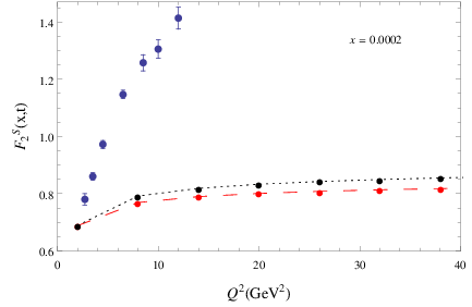
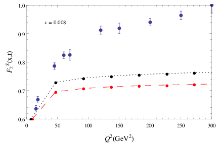
In the expressions a2​(x,t,0.8)a_{2}(x,t,0.8) and a4​(x,t,0.8)a_{4}(x,t,0.8) there is an integration over xx.So to obtain it numerically a lower and upper limit of xx is required.We take the lower limit of xx as 6×10−76\times 10^{-7} [6] and upper limit as 0.20.2.Our model is based on small xx so the highest limit we take here is 0.2 which is the plausible higher small xx limit. We test graphically whether the structure functions F2S⁡(I)​(x,t)F_{2}^{S(I)}(x,t) and F2S⁡(I​I)​(x,t)F_{2}^{S(II)}(x,t) obtained from equations (49) and (50) using equations(57) and (58) respectively match well with the recent HERA data as in Fig.1.
Refer to caption
(a)
Refer to caption
(b)
Figure 1: Plot of Singlet Structure Function F2S​(x,t)F_{2}^{S}(x,t) as a function of Q2Q^{2} at different fixed xx with HERAPDF1.0 data.Here the red dashed-connected line represents our analytical result for F2S⁡(I)​(x,t)F_{2}^{S(I)}(x,t) and that of black dotted- connected line for F2S⁡(I​I)​(x,t)F_{2}^{S(II)}(x,t),obtained by Lagrange’s Auxiliary method .

We observe that the two solutions (57) and (58) have different Q2Q^{2} evolutions and second solution is much closer to the experimental data.

3.2 For O⁡(x2)O(x^{2}):

We assume that for a very small xx ,we can take sin⁡β​x≃0\sin\beta x\simeq 0 in equation(34)

qI​(x,t)=exp⁡[−s2​631​(1t−1t0)].[eα​x​(c1​cos⁡β​x)]q^{I}(x,t)=\exp[-s^{2}\frac{6}{31}(\frac{1}{t}-\frac{1}{t_{0}})].\left[e^{\alpha x}(c_{1}\cos\beta x)\right] (59)

Likewise as in O⁡(x)O(x)

qI​(x,t)=qI​(x,t0)​qI​(x,t)qI​(x,t0)q^{I}(x,t)=q^{I}(x,t_{0})\frac{q^{I}(x,t)}{q^{I}(x,t_{0})} (60)

Now,

qI​(x,t)qI​(x,t0)=exp⁡[−s2​631​(1t−1t0)].[eα​x​(c1​cos⁡β​x)][eα​x​(c1​cos⁡β​x)]\frac{q^{I}(x,t)}{q^{I}(x,t_{0})}=\frac{\exp[-s^{2}\frac{6}{31}(\frac{1}{t}-\frac{1}{t_{0}})].\left[e^{\alpha x}(c_{1}\cos\beta x)\right]}{\left[e^{\alpha x}(c_{1}\cos\beta x)\right]} (61)

Putting in equation(60) we obtain,

qI​(x,t)=q⁡(x,t0)​exp⁡[−s2​631​(1t−1t0)]q^{I}(x,t)=q(x,t_{0})\exp[-s^{2}\frac{6}{31}(\frac{1}{t}-\frac{1}{t_{0}})] (62)

Similarly for qI​I​(x,t)q^{II}(x,t) of equation(37) when sin⁡β^​x≃0\sin\hat{\beta}x\simeq 0

qI​I​(x,t)=q⁡(x,t0)​exp⁡[−s^2​631​k​(1t−1t0)]q^{II}(x,t)=q(x,t_{0})\exp[-\hat{s}^{2}\frac{6}{31k}(\frac{1}{t}-\frac{1}{t_{0}})] (63)

where in equations (62) and (63) we assumed qI​(x,t0)=qI​I​(x,t0)=q⁡(x,t0)q^{I}(x,t_{0})=q^{II}(x,t_{0})=q(x,t_{0}) (input distribution).
In terms of Singlet Structure Function we get,

F2S⁡(I)​(x,t)=F2S​(x,t0)​exp⁡[−s2​631​(1t−1t0)]\displaystyle F_{2}^{S(I)}(x,t)=F_{2}^{S}(x,t_{0})\exp[-s^{2}\frac{6}{31}(\frac{1}{t}-\frac{1}{t_{0}})] (64)

Again,

F2S⁡(I​I)​(x,t)=F2S​(x,t0)​exp⁡[−s^2​631​k​(1t−1t0)]\displaystyle F_{2}^{S(II)}(x,t)=F_{2}^{S}(x,t_{0})\exp[-\hat{s}^{2}\frac{6}{31k}(\frac{1}{t}-\frac{1}{t_{0}})] (65)

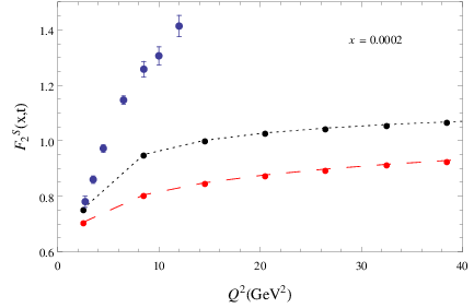
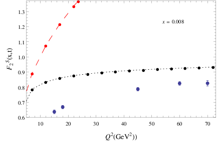
Now we make a graphical interpretation of our obtained Singlet Structure Functions as a function of Q2Q^{2} for a certain xx.We use the obtained value of kk as in O⁡(x)O(x) as 0.8 and we take separation constants s2=5s^{2}=5 and s^2=5\hat{s}^{2}=5, as lower the value of separation constants makes the separation between the F2S⁡(I)​(x,t)F_{2}^{S(I)}(x,t) and F2S⁡(I​I)​(x,t)F_{2}^{S(II)}(x,t) plots less.

Refer to caption
(a)
Refer to caption
(b)
Figure 2: Plot of Singlet Structure Function F2S​(x,t)F_{2}^{S}(x,t) as a function of Q2Q^{2} at different fixed xx with HERAPDF1.0 data.Here the red dashed-connected line represents our analytical result for F2S⁡(I)​(x,t)F_{2}^{S(I)}(x,t) and that of black dotted- connected line for F2S⁡(I​I)​(x,t)F_{2}^{S(II)}(x,t), obtained by the method of Separation of Variables.

Fig.2(a) and fig.2(b) have the same feature as in fig.1(a) and fig.1(b) which shows the non identical nature of solutions and the second solution is closer to the data.

4 Conclusion

In this paper we have shown that the two solutions qI​(x,t)q^{I}(x,t) and qI​I​(x,t)q^{II}(x,t) obtained from the DGLAP equations (13) and (14) for O⁡(x)O(x) and from equations (15) and (16) for O⁡(x2)O(x^{2}) are not identical with each other,a feature not studied in the earlier communications [7, 9, 8, 15].The graphical representations also support this conclusion.While comparing with the recent HERA data, we find that our theoretical prediction of first solution overshoots the experimental data and the second one is much closer to it. Proper incorporation of flavour dependence in the equations (12) and (48) might perhaps improve our result further significantly.Such study is currently under progress.

Acknowledgment

One of the authors (L.M) acknowledges the Rajiv Gandhi National Fellowship, New Delhi for financial support.

References

  • [1] V. N. Gribov and L. N. Lipatov, Sov. J. Nucl. Phys., 15, 438 (1972);
  • [2] L. N. Lipatov, Sov. J. Nucl. Phys., 20, 94 (1975);
  • [3] Yu. L. Dokshitzer, Sov. Phys. JETP, 46, 641 (1977);
  • [4] G. Altarelli and G. Parisi, Nucl. Phys. B126, 298 (1977);
  • [5] QCD and collider Physics,R.K Ellis,W.J Stirling and B.R.Webber
  • [6] H1 and ZEUS Collaborations (Aaron, F.D. et al.) JHEP 1001 (2010) 109 arXiv:0911.0884 [hep-ex] DESY-09-158
  • [7] D.K. Choudhury and J.K. Sarma, Pramana J. Phys.,Vol.38, No.5, May 1992, pp.481-489.
  • [8] J. K. Sarma, D. K. Choudhury and G. K. Medhi, Phys. Lett. B403, 139 (1997).
  • [9] Neelakshi N.K. Borah, D.K. Choudhury and P.K. Sahariah, Advances in High Energy Physics Volume 2013 Article ID 829803, 10 pages.
  • [10] I. Sneddon,(1957)p131; Elements of Partial Differential Equations,M.Graw Hill, NewYork
  • [11] A.B. Gupta,(2004)p381; Fundamentals of Mathematical Physics,Books and Allied (P) LTD,Kolkata;
  • [12] D.K Choudhury Journal of Physics,Conference series 481(2014)012021
  • [13] A. Jahan and D.K. Choudhury, Commun.Theor. Phys. 61(2014) 654-658
  • [14] C. Lopez and F. J. Yndurain, Nucl. Phys. B171, 231 (1980).
  • [15] D.K. Choudhury and Neelakshi N.K. Borah arXiv:1508.06041v3 [hep-ph] 14 May 2016 accepted for publication in Physical Review D.

Appendix A:

J1​(x)=∫x1d​zz​CF​{(1+z2)(1−z)++32​δ​(1−z)}​J2​(x)=∫x1d​zz​∑r=1∞ur​CF​{(1+z2)(1−z)++32​δ​(1−z)}​J3​(x)=∫x1d​zz​(∑r=1∞ur)22!​CF​{(1+z2)(1−z)++32​δ​(1−z)}​J4​(x)=∫x1d​zz​TR​{z2+(1−z)2}​J5​(x)=∫x1d​zz​TR​{z2+(1−z)2}​∑r=1∞ur​J6​(x)=∫x1d​zz​TR​{z2+(1−z)2}​(∑r=1∞ur)22!​J7​(x)=∫x1d​zz​CF​{(1+(1−z)2)z}​J8​(x)=∫x1d​zz​CF​{(1+(1−z)2)z}​∑r=1∞ur​J9​(x)=∫x1d​zz​CF​{(1+(1−z)2)z}​(∑r=1∞ur)22!​J10​(x)=∫x1d​zz​{2​CA​(z(1−z)++1−zz+z⁡(1−z))+δ⁡(1−z)​11​CA−4​Nf​TR6}​J11​(x)=∫x1d​zz​{2​CA​(z(1−z)++1−zz+z⁡(1−z))+δ⁡(1−z)​11​CA−4​Nf​TR6}​∑r=1∞ur​J12​(x)=∫x1d​zz​{2​CA​(z(1−z)++1−zz+z⁡(1−z))+δ⁡(1−z)​11​CA−4​Nf​TR6}​(∑r=1∞ur)22!J_{1}(x)=\int_{x}^{1}\frac{dz}{z}C_{F}\left\{\frac{(1+z^{2})}{(1-z)_{+}}+\frac{3}{2}\delta(1-z)\right\}\\ J_{2}(x)=\int_{x}^{1}\frac{dz}{z}\sum_{r=1}^{\infty}u^{r}C_{F}\left\{\frac{(1+z^{2})}{(1-z)_{+}}+\frac{3}{2}\delta(1-z)\right\}\\ J_{3}(x)=\int_{x}^{1}\frac{dz}{z}\frac{(\sum_{r=1}^{\infty}u^{r})^{2}}{2!}C_{F}\left\{\frac{(1+z^{2})}{(1-z)_{+}}+\frac{3}{2}\delta(1-z)\right\}\\ J_{4}(x)=\int_{x}^{1}\frac{dz}{z}T_{R}\left\{z^{2}+(1-z)^{2}\right\}\\ J_{5}(x)=\int_{x}^{1}\frac{dz}{z}T_{R}\left\{z^{2}+(1-z)^{2}\right\}\sum_{r=1}^{\infty}u^{r}\\ J_{6}(x)=\int_{x}^{1}\frac{dz}{z}T_{R}\left\{z^{2}+(1-z)^{2}\right\}\frac{(\sum_{r=1}^{\infty}u^{r})^{2}}{2!}\\ J_{7}(x)=\int_{x}^{1}\frac{dz}{z}C_{F}\left\{\frac{(1+(1-z)^{2})}{z}\right\}\\ J_{8}(x)=\int_{x}^{1}\frac{dz}{z}C_{F}\left\{\frac{(1+(1-z)^{2})}{z}\right\}\sum_{r=1}^{\infty}u^{r}\\ J_{9}(x)=\int_{x}^{1}\frac{dz}{z}C_{F}\left\{\frac{(1+(1-z)^{2})}{z}\right\}\frac{(\sum_{r=1}^{\infty}u^{r})^{2}}{2!}\\ J_{10}(x)=\int_{x}^{1}\frac{dz}{z}\left\{2C_{A}\left(\frac{z}{(1-z)_{+}}+\frac{1-z}{z}+z(1-z)\right)+\delta(1-z)\frac{11C_{A}-4N_{f}T_{R}}{6}\right\}\\ J_{11}(x)=\int_{x}^{1}\frac{dz}{z}\left\{2C_{A}\left(\frac{z}{(1-z)_{+}}+\frac{1-z}{z}+z(1-z)\right)+\delta(1-z)\frac{11C_{A}-4N_{f}T_{R}}{6}\right\}\sum_{r=1}^{\infty}u^{r}\\ J_{12}(x)=\int_{x}^{1}\frac{dz}{z}\left\{2C_{A}\left(\frac{z}{(1-z)_{+}}+\frac{1-z}{z}+z(1-z)\right)+\delta(1-z)\frac{11C_{A}-4N_{f}T_{R}}{6}\right\}\frac{(\sum_{r=1}^{\infty}u^{r})^{2}}{2!}

Appendix B:

X1(x,t)=exp[−∫d​xP1​(x,t)]Y1(x,t)=exp[−∫d​xP1​(x,t)R^1(x,t)]X2(x,t)=exp[−∫d​xP2​(x,t)−∫d​tt​C​(t)]Y2(x,t)=exp[−∫d​xP2​(x,t)R^2(x,t)]Q1(x,t)=tP1(x,t)=−αs​(t)2​πx[J2(x)+J5(x)C(x,t)]R1(x,t)=αs​(t)2​π[J1(x)+J4(x)C(x,t)]q(x,t)=R1^(x,t)q(x,t)Q2(x,t)=tC(t)P2(x,t)=−αs​(t)2​πx[J8(x)+J11(x)C(x,t)]R2(x,t)=[αs​(t)2​π{J7(x)+J10(x)C(x,t)}−t∂∂tC(x,t)]q(x,t)=R2^(x,t)q(x,t)X_{1}(x,t)=exp\left[-\int\frac{dx}{P_{1}(x,t)}\right]\\ Y_{1}(x,t)=exp\left[-\int\frac{dx}{P_{1}(x,t)}\hat{R}_{1}(x,t)\right]\\ X_{2}(x,t)=exp\left[-\int\frac{dx}{P_{2}(x,t)}-\int\frac{dt}{tC(t)}\right]\\ Y_{2}(x,t)=exp\left[-\int\frac{dx}{P_{2}(x,t)}\hat{R}_{2}(x,t)\right]\\ Q_{1}(x,t)=t\\ P_{1}(x,t)=-\frac{\alpha_{s}(t)}{2\pi}x[J_{2}(x)+J_{5}(x)C(x,t)]\\ R_{1}(x,t)=\frac{\alpha_{s}(t)}{2\pi}[J_{1}(x)+J_{4}(x)C(x,t)]q(x,t)=\hat{R_{1}}(x,t)q(x,t)\\ Q_{2}(x,t)=tC(t)\\ P_{2}(x,t)=-\frac{\alpha_{s}(t)}{2\pi}x[J_{8}(x)+J_{11}(x)C(x,t)]\\ R_{2}(x,t)=[\frac{\alpha_{s}(t)}{2\pi}\left\{J_{7}(x)+J_{10}(x)C(x,t)\right\}-t\frac{\partial}{\partial t}C(x,t)]q(x,t)=\hat{R_{2}}(x,t)q(x,t)\\

Appendix C:

a1​(x,k)=1α1exp(−∫αs​(t)2​π​(J1​(x)+J4​(x)​k)−αs​(t)2​π​x​(J2​(x)+J5​(x)​k)dx)a_{1}(x,k)=\frac{1}{\alpha_{1}\exp\left(-\int\frac{\frac{\alpha_{s}(t)}{2\pi}(J_{1}(x)+J_{4}(x)k)}{-\frac{\alpha_{s}(t)}{2\pi}x(J_{2}(x)+J_{5}(x)k)}dx\right)}
a2(x,k)=−∫d​x−αs​(t)2​π​x​(J2​(x)+J5​(x)​k)a_{2}(x,k)=-\int\frac{dx}{-\frac{\alpha_{s}(t)}{2\pi}x(J_{2}(x)+J_{5}(x)k)}
a3​(x,k)=1α2exp(−∫αs​(t)2​π​(J7​(x)+J10​(x)​k)−αs​(t)2​π​x​(J8​(x)+J11​(x)​k)dx)a_{3}(x,k)=\frac{1}{\alpha_{2}\exp\left(-\int\frac{\frac{\alpha_{s}(t)}{2\pi}(J_{7}(x)+J_{10}(x)k)}{-\frac{\alpha_{s}(t)}{2\pi}x(J_{8}(x)+J_{11}(x)k)}dx\right)}
a4(x,k)=−∫d​x−αs​(t)2​π​x​(J8​(x)+J11​(x)​k)−1klog(t)a_{4}(x,k)=-\int\frac{dx}{-\frac{\alpha_{s}(t)}{2\pi}x(J_{8}(x)+J_{11}(x)k)}-\frac{1}{k}log(t)

Appendix D:

For different inputs qI​(x,t)q^{I}(x,t) and qI​I​(x,t)q^{II}(x,t) will evolve differently.For q⁡(x,t0)q(x,t_{0}) we take the input parameterization of HERA group at Q02=1.9Q_{0}^{2}=1.9 GeV2 as follows.

x​uv​(x)=Auv​xBuv​(1−x)Cuv​(1+Euv​x2)xu_{v}(x)=A_{u_{v}}x^{B_{u_{v}}}(1-x)^{C_{u_{v}}}(1+E_{u_{v}}x^{2})
x​dv​(x)=Adv​xBdv​(1−x)Cdvxd_{v}(x)=A_{d_{v}}x^{B_{d_{v}}}(1-x)^{C_{d_{v}}}
x​U¯​(x)=AU¯​xBU¯​(1−x)CU¯x\bar{U}(x)=A_{\bar{U}}x^{B_{\bar{U}}}(1-x)^{C_{\bar{U}}}
x​D¯​(x)=AD¯​xBD¯​(1−x)CD¯x\bar{D}(x)=A_{\bar{D}}x^{B_{\bar{D}}}(1-x)^{C_{\bar{D}}}

The values of the parameters Auv,Buv,Cuv,EuvA_{u_{v}},B_{u_{v}},C_{u_{v}},E_{u_{v}} etc are as given in Appendix C Table1.

If x​U,x​D,x​U¯xU,xD,x\bar{U} and x​D¯x\bar{D} denote the sums of up,down and their corresponding anti-quark distributions respectively and are related to quark distributions as:

x​U=x​u+x​cxU=xu+xc
x​U¯=x​u¯+x​c¯x\bar{U}=x\bar{u}+x\bar{c}
x​D=x​d+x​sxD=xd+xs
x​D¯=x​d¯+x​s¯x\bar{D}=x\bar{d}+x\bar{s}

x​s,x​cxs,xc are strange and charm quark distributions. Assuming sea quarks and anti-quarks symmetry yields the valence quark distributions as

x​uv=x​U−x​U¯xu_{v}=xU-x\bar{U}
x​dv=x​D−x​D¯xd_{v}=xD-x\bar{D}

Now the singlet structure function F2S​(x)F_{2}^{S}(x) for the three flavors u,d,su,d,s is:

F2S​(x)=x⁡{u⁡(x)+u¯​(x)}+x⁡{d⁡(x)+d¯​(x)}+x⁡{s⁡(x)+s¯​(x)}F_{2}^{S}(x)=x\left\{u(x)+\bar{u}(x)\right\}+x\left\{d(x)+\bar{d}(x)\right\}+x\left\{s(x)+\bar{s}(x)\right\}

Where u⁡(x)=uv​(x)+us​(x)u(x)=u_{v}(x)+u_{s}(x) and so for d⁡(x)d(x) and s⁡(x)s(x).uv​(x)u_{v}(x) and us​(x)u_{s}(x) are the uu valence and uu sea quark distributions respectively and we assume us≈ds≈ss≈u¯s≈d¯s≈s¯su_{s}\approx d_{s}\approx s_{s}\approx\bar{u}_{s}\approx\bar{d}_{s}\approx\bar{s}_{s} for x→0x\rightarrow 0, So the singlet structure function becomes

F2S​(x)=x​uv​(x)+x​dv​(x)+6​x​ss​(x)F_{2}^{S}(x)=xu_{v}(x)+xd_{v}(x)+6xs_{s}(x)
⟹F2S​(x)=x​uv​(x)+x​dv​(x)+3​x​D¯​(x)\implies F_{2}^{S}(x)=xu_{v}(x)+xd_{v}(x)+3x\bar{D}(x)

We take two data points for a fixed xx and two different Q2Q^{2} 150 GeV2 and 200 GeV2 and their corresponding parton distribution data values [6].
For x=0.800×10⁻²,Q2=150x=0.800\times 10^{-2},Q^{2}=150 GeV2,F2S​(x,t)=0.919F_{2}^{S}(x,t)=0.919 and t0=t_{0}=logQ02Λ2\frac{Q_{0}^{2}}{\Lambda^{2}}, Nf=3N_{f}=3,Λ(3)=340\Lambda^{(3)}=340MeV, F2S​(x,t0)=x​q​(x,t0)=0.578639F_{2}^{S}(x,t_{0})=xq(x,t_{0})=0.578639 we obtain an equation interms of β1\beta_{1} and kk from equation(55) as

0.58821​β1−4.44615×exp⁡(0.6046868+3​k)+7.16825×exp⁡(1.548348+3​k)=00.58821\beta_{1}-4.44615\times\exp(\frac{0.604686}{8+3k})+7.16825\times\exp(\frac{1.54834}{8+3k})=0 (66)

Likewise for x=0.800×10⁻²,Q2=200x=0.800\times 10^{-2},Q^{2}=200 GeV2,F2S​(x,t)=0.940F_{2}^{S}(x,t)=0.940, we obtain from equation(55) as

0.6245​β1−4.54774×exp⁡(0.6046868+3​k)+7.45594×exp⁡(1.610488+3​k)=00.6245\beta_{1}-4.54774\times\exp(\frac{0.604686}{8+3k})+7.45594\times\exp(\frac{1.61048}{8+3k})=0 (67)

From eqn(66) we can write as

β1=7.55878×exp⁡(0.6046868+3​k)−12.1865×exp⁡(1.548348+3​k)\beta_{1}=7.55878\times\exp(\frac{0.604686}{8+3k})-12.1865\times\exp(\frac{1.54834}{8+3k})

and use it in the equation(67) which yields as

0.17×exp⁡(0.608+3​k)−7.61×exp⁡(1.548+3​k)+7.45×exp⁡(1.618+3​k)=00.17\times\exp(\frac{0.60}{8+3k})-7.61\times\exp(\frac{1.54}{8+3k})+7.45\times\exp(\frac{1.61}{8+3k})=0 (68)

To make our mathematics simpler we assume the expansion series of exe^{x} upto the first order of xx in ex=1+x1!+x22!+…e^{x}=1+\frac{x}{1!}+\frac{x^{2}}{2!}+... and incorporate in the above equation(68) and we obtain the value of kk as 0.8 and henceforth we obtain the value of β1\beta_{1} as -6.03 from equation(67) and β2\beta_{2} to be 0.57 from equation(56) with x=0.800×10⁻²,Q2=150x=0.800\times 10^{-2},Q^{2}=150 GeV2,F2S​(x,t)=0.919F_{2}^{S}(x,t)=0.919

Table 1: Cental values of the HERAPDF1.0 parameters
AA BB CC EE
x​gxg 6.8 0.22 9.0
x​uvxu_{v} 3.7 0.67 4.7 9.7
x​dvxd_{v} 2.2 0.67 4.3
x​U¯x\bar{U} 0.113 -0.165 2.6
x​D¯x\bar{D} 0.163 -0.165 2.4