跳到论文正文
W Papers独立论文阅读器 arXiv:1612.08263 论文正文 计算阅读时间 · 0%
引用这篇论文根据当前论文元数据生成,正式投稿前建议核对。


License: arXiv.org perpetual non-exclusive license
arXiv:1612.08263v3 [eess.SY] 13 Jan 2018

Decentralized RLS with Data-Adaptive Censoring for Regressions over Large-Scale NetworksThanks: Zifeng Wang and Zheng Yu are with the Special Class for the Gifted Young, University of Science and Technology of China. Emails: wzfeng@mail.ustc.edu.cn and yz123@mail.ustc.edu.cn. Qing Ling (corresponding author) is with the School of Data and Computer Science, Sun Yat-Sen University. Email: lingqing556@mail.sysu.edu.cn. Dimitris Berberidis and Georgios B. Giannakis are with the Dept. of ECE, University of Minnesota. Emails: bermp001@umn.edu and georgios@umn.edu. This work was supported by NSF China grant 61573331, NSF Anhui grant 1608085QF130, NSF grants 1442686, 1500713, and 1711471. Part of this paper has appeared at the 42nd Intl. Conf. on Acoustics, Speech, and Signal Processing, New Orleans, USA, March 5–9, 2017 [28].

Zifeng Wang, Zheng Yu, Qing Ling, Dimitris Berberidis, and Georgios B. Giannakis Affiliation: 
Abstract

The deluge of networked data motivates the development of algorithms for computation- and communication-efficient information processing. In this context, three data-adaptive censoring strategies are introduced to considerably reduce the computation and communication overhead of decentralized recursive least-squares (D-RLS) solvers. The first relies on alternating minimization and the stochastic Newton iteration to minimize a network-wide cost, which discards observations with small innovations. In the resultant algorithm, each node performs local data-adaptive censoring to reduce computations, while exchanging its local estimate with neighbors so as to consent on a network-wide solution. The communication cost is further reduced by the second strategy, which prevents a node from transmitting its local estimate to neighbors when the innovation it induces to incoming data is minimal. In the third strategy, not only transmitting, but also receiving estimates from neighbors is prohibited when data-adaptive censoring is in effect. For all strategies, a simple criterion is provided for selecting the threshold of innovation to reach a prescribed average data reduction. The novel censoring-based (C)D-RLS algorithms are proved convergent to the optimal argument in the mean-root deviation sense. Numerical experiments validate the effectiveness of the proposed algorithms in reducing computation and communication overhead.

Index Terms: 
Decentralized estimation, networks, recursive least-squares (RLS), data-adaptive censoring

I Introduction

In our big data era, various networks generate massive amounts of streaming data. Examples include wireless sensor networks, where a large number of inexpensive sensors cooperate to monitor, e.g. the environment [21, 22], or data centers, where a group of servers collaboratively handles dynamic user requests [24]. Since a single node has limited computational resources, decentralized information processing is preferable as the network size scales up [7, 9]. In this paper, we focus on a decentralized linear regression setup, and develop computation- and communication-efficient decentralized recursive least-squares (D-RLS) algorithms.

The main tool we adopt to reduce computation and communication costs is data-adaptive censoring, which leverages the redundancy present especially in big data. Upon receiving an observation, nodes determine whether it is informative or not. Less informative observations are discarded, while messages among neighboring nodes are exchanged only when necessary. We propose three censoring-based (C)D-RLS algorithms that can achieve estimation accuracy comparable to D-RLS without censoring, while significantly reducing the computation and communication overhead.

I-A Related works

The merits of RLS algorithms in solving centralized linear regression problems are well recognized [12, 25]. When streaming observations that depend linearly on a set of unknown parameters become available, RLS yields the least-squares parameter estimates online. RLS reduces the computational burden of finding a batch estimate per iteration, and can even allow for tracking time-varying parameters. The computational cost can be further reduced by data-adaptive censoring [4], where less informative data are discarded. On the other hand, decentralized versions of RLS without censoring have been advocated to solve linear regression tasks over networks [16]. In D-RLS, a node updates its estimate that is common to the entire network by fusing its local observations with the local estimates of its neighbors. As time evolves, all local estimates consent on the centralized RLS solution. This paper builds on both [4] and [16] by developing censoring-based decentralized RLS algorithms, thus catering to efficient online linear regression over large-scale networks.

Different from our in-network setting where operation is fully decentralized and nodes are only able to communicate with their neighbors, most of the existing distributed censoring algorithms apply to star topology networks that rely on a fusion center [2, 10, 11, 19, 23]. Their basic idea is that each node transmits data to the fusion center for further processing only when its local likelihood ratio exceeds a threshold [23]; see also [10] where communication constraints are also taken into account. Information fusion over fading channels is considered in [11]. Practical issues such as joint dependence of sensor decision rules, randomization of decision strategies as well as partially known distributions are reported in [2], while [19] also explores quantization jointly with censoring.

Other than the star topology studied in the aforementioned works, [20] investigates censoring for a tree structure. If a node’s local likelihood ratio exceeds a threshold, its local data is sent to its parent node for fusion. A fully decentralized setting is considered in [3], where each node determines whether to transmit its local estimate to its neighbors by comparing the local estimate with the weighted average of its neighbors. Nevertheless, [3] aims at mitigating only the communication cost, while the present work also considers reduction of the computational cost across the network. Furthermore, the censoring-based decentralized linear regression algorithm in [14] deals with optimal full-complexity estimation when observations are partially known or corrupted. This is different from our context, where censoring is deliberately introduced to reduce computational and communication costs for decentralized linear regression.

I-B Our contributions and organization

The present paper introduces three data-adaptive online censoring strategies for decentralized linear regression. The resultant CD-RLS algorithms incur low computational and communication costs, and are thus attractive for large-scale network applications requiring decentralized solvers of linear regressions. Unlike most related works that specifically target wireless sensor networks (WSNs), the proposed algorithms may be used in a broader context of decentralized linear regression using multiple computing platforms. Of particular interest are cases where a regression dataset is not available at a single machine, but it is distributed over a network of computing agents that are interested in accurately estimating the regression coefficients in an efficient manner.

In Section II, we formulate the decentralized online linear regression problem (Section II-A), and recast the D-RLS in [16] into a new form (Section II-B) that prompts the development of three censoring strategies (Section II-C). Section III develops the first censoring strategy (Section III-A), analyzes all three censoring strategies (Section III-B), and discusses how to set the censoring thresholds (Section III-C). Numerical experiments in Section IV demonstrate the effectiveness of the novel CD-RLS algorithms.

Notation. Lower (upper) case boldface letters denote column vectors (matrices). (⋅)T(\cdot)^{T}, ||⋅||||\cdot||, ||⋅||2||\cdot||_{2} and E⁡[⋅]E[\cdot] stand for transpose, 2-norm, induced matrix 2-norm and expectation, respectively. Symbols tr⁡(𝐗)\mathrm{tr}(\mathbf{X}), λmin​(𝐗)\lambda_{\text{min}}(\mathbf{X}) and λmax​(𝐗)\lambda_{\text{max}}(\mathbf{X}) are used for the trace, minimum eigenvalue and maximal eigenvalue of matrix 𝐗\mathbf{X}, respectively. Kronecker product is denoted by ⊗\otimes and the uniform distribution over [a,b][a,b] by 𝒰⁡(a,b)\mathcal{U}(a,b), and the Gaussian probability distribution function (pdf) with mean μ\mu and variance σ2\sigma^{2} by 𝒩⁡(μ,σ2)\mathcal{N}(\mu,\sigma^{2}). The standardized Gaussian pdf is ϕ(t)=(1/2​π)exp(−t2/2)\phi(t)=(1/\sqrt{2\pi})\text{exp}(-t^{2}/2), and its the associated complementary cumulative distribution function is represented by Q⁡(z):=∫z+∞ϕ⁡(t)​𝑑tQ(z):=\int_{z}^{+\infty}\phi(t)dt.

II Context and Algorithms

This section outlines the online linear regression setup over networks, and takes a fresh look at the D-RLS algorithm. Three strategies are then developed using data-adaptive censoring to reduce the computational and communication costs of D-RLS.

II-A Problem statement

Consider a bidirectionally connected network with JJ nodes, described by a graph 𝒢:={𝒱,ℰ}\mathcal{G}:=\{\mathcal{V},\mathcal{E}\}, where 𝒱\mathcal{V} is the set of nodes with cardinality |𝒱|=J|\mathcal{V}|=J, and ℰ\mathcal{E} denotes the set of edges. Each node jj only communicates with its one-hop neighbors, collected in the set 𝒩j⊂𝒱\mathcal{N}_{j}\subset\mathcal{V}. The decentralized network is deployed to estimate a real vector 𝐬0∈ℝp{\mathbf{s}}_{0}\in{\mathbb{R}}^{p}. Per time slot t=1,2,…t=1,2,\ldots, node jj receives a real scalar observation xj​(t)x_{j}(t) involving the wanted 𝐬0{\mathbf{s}}_{0} with a regression row 𝐡jT​(t)\mathbf{h}_{j}^{T}(t), so that xj​(t)=𝐡jT​(t)​𝐬0+ϵj​(t)x_{j}(t)=\mathbf{h}_{j}^{T}(t){\mathbf{s}}_{0}+\epsilon_{j}(t), with ϵj​(t)∼𝒩⁡(0,σj2)\epsilon_{j}(t)\sim\mathcal{N}(0,\sigma_{j}^{2}).

Our goal is to devise efficient decentralized online algorithms to solve the following exponentially-weighted least-squares (EWLS) problem

𝐬^e​w​l​s​(t):=arg⁡min𝐬​12​∑r=1t∑j=1Jλt−r​[xj​(r)−𝐡jT​(r)​𝐬]2\displaystyle\hat{{\mathbf{s}}}_{ewls}(t):=\arg\min\limits_{{\mathbf{s}}}\frac{1}{2}~\sum_{r=1}^{t}\sum_{j=1}^{J}\lambda^{t-r}[x_{j}(r)-\mathbf{h}_{j}^{T}(r){\mathbf{s}}]^{2} (1)

where 𝐬^e​w​l​s​(t)\hat{{\mathbf{s}}}_{ewls}(t) is the EWLS estimate at slot tt, and λ∈(0,1]\lambda\in(0,1] is a forgetting factor that de-emphasizes the importance of past measurements, and thus enables tracking of a non-stationary process. When λ=1\lambda=1, (1) boils down to a standard decentralized online least-squares estimate.

II-B D-RLS revisited

The D-RLS algorithm of [16] solves (1) as follows. Per time slot tt, node jj receives xj​(t)x_{j}(t) and 𝐡jT​(t)\mathbf{h}_{j}^{T}(t) and uses them to update the per-node inverse p×pp\times p covariance matrix as

𝚽j−1​(t)\displaystyle\mathbf{\Phi}_{j}^{-1}(t) =λ−1​𝚽j−1​(t−1)\displaystyle=\lambda^{-1}\mathbf{\Phi}_{j}^{-1}(t-1)
−λ−1​𝚽j−1​(t−1)​𝐡j​(t)​𝐡jT​(t)​𝚽j−1​(t−1)λ+𝐡jT​(t)​𝚽j−1​(t−1)​𝐡j​(t)\displaystyle-\frac{\lambda^{-1}\mathbf{\Phi}_{j}^{-1}(t-1)\mathbf{h}_{j}(t)\mathbf{h}_{j}^{T}(t)\mathbf{\Phi}_{j}^{-1}(t-1)}{\lambda+\mathbf{h}_{j}^{T}(t)\mathbf{\Phi}_{j}^{-1}(t-1)\mathbf{h}_{j}(t)} (2)

along with the per-node p×1p\times 1 cross-covariance vector as

𝝍j​(t)\displaystyle\bm{\psi}_{j}(t) =λ​𝝍j​(t−1)+𝐡j​(t)​xj​(t).\displaystyle=\lambda\bm{\psi}_{j}(t-1)+\mathbf{h}_{j}(t)x_{j}(t). (3)

Using 𝚽j−1​(t)\mathbf{\Phi}_{j}^{-1}(t) and 𝝍j​(t)\bm{\psi}_{j}(t), node jj then updates its local parameter estimate using

𝐬j​(t)=𝚽j−1​(t)​[𝝍j​(t)−12​∑j′∈𝒩j(𝐯jj′​(t−1)−𝐯j′j​(t−1))]\displaystyle{\mathbf{s}}_{j}(t)=\mathbf{\Phi}_{j}^{-1}(t)\Big[\bm{\psi}_{j}(t)-\frac{1}{2}\sum_{j^{\prime}\in\mathcal{N}_{j}}\left({\mathbf{v}}_{j}^{j^{\prime}}(t-1)-{\mathbf{v}}_{j^{\prime}}^{j}(t-1)\right)\Big] (4)

where 𝐯jj′​(t−1){\mathbf{v}}_{j}^{j^{\prime}}(t-1) denotes the Lagrange multiplier of node jj corresponding to its neighbor j′j^{\prime} at slot t−1t-1, that captures the accumulated differences of neighboring estimates, recursively obtained as (ρ>0\rho>0 is a step-size)

𝐯jj′​(t−1)=𝐯jj′​(t−2)+ρ⁡[𝐬j​(t−1)−𝐬j′​(t−1)].\displaystyle{\mathbf{v}}_{j}^{j^{\prime}}(t-1)={\mathbf{v}}_{j}^{j^{\prime}}(t-2)+\rho\big[{\mathbf{s}}_{j}(t-1)-{\mathbf{s}}_{j^{\prime}}(t-1)\big]. (5)

Next, we develop an equivalent novel form of D-RLS recursions (2)–(5) that is convenient for our incorporation of data-adaptive censoring. Detailed derivation of the equivalence can be found in Appendix A. The inverse covariance matrix is updated as in (2). However, the update of 𝐬j​(t){\mathbf{s}}_{j}(t) in (4) is replaced by

𝐬j​(t)\displaystyle{\mathbf{s}}_{j}(t) =𝐬j​(t−1)+𝚽j−1​(t)​𝐡j​(t)​[xj​(t)−𝐡jT​(t)​𝐬j​(t−1)]\displaystyle={\mathbf{s}}_{j}(t-1)+\mathbf{\Phi}_{j}^{-1}(t)\mathbf{h}_{j}(t)\big[x_{j}(t)-\mathbf{h}_{j}^{T}(t){\mathbf{s}}_{j}(t-1)\big]
−ρ​𝚽j−1​(t)​𝜹j​(t−1)\displaystyle-\rho\mathbf{\Phi}_{j}^{-1}(t)\bm{\delta}_{j}(t-1) (6)

where 𝜹j​(t)\bm{\delta}_{j}(t) stands for a Lagrange multiplier conveying network-wide information that is updated as

𝜹j​(t)\displaystyle\bm{\delta}_{j}(t) =𝜹j​(t−1)+∑j′∈𝒩j[𝐬j​(t)−𝐬j′​(t)]\displaystyle=\bm{\delta}_{j}(t-1)+\sum_{j^{\prime}\in\mathcal{N}_{j}}[{\mathbf{s}}_{j}(t)-{\mathbf{s}}_{j^{\prime}}(t)]
−λ∑j′∈𝒩j[𝐬j(t−1)−𝐬j′(t−1)].\displaystyle-\lambda\sum_{j^{\prime}\in\mathcal{N}_{j}}[{\mathbf{s}}_{j}(t-1)-{\mathbf{s}}_{j^{\prime}}(t-1)]. (7)

Observe that 𝜹j​(t)\bm{\delta}_{j}(t) stores the weighted sum of differences between the local estimate of node jj, and all estimates of its neighbors. Interestingly, if the network is disconnected and the nodes are isolated, then 𝜹j​(t)=𝟎\bm{\delta}_{j}(t)=\mathbf{0} so long as 𝜹j​(0)=𝟎\bm{\delta}_{j}(0)=\mathbf{0}, and the update of 𝐬j​(t){\mathbf{s}}_{j}(t) in (6) basically boils down to the centralized RLS one [12, 25]. That is, the current estimate is modified from its previous value using the prediction error xj​(t)−𝐡jT​(t)​𝐬j​(t−1)x_{j}(t)-\mathbf{h}_{j}^{T}(t){\mathbf{s}}_{j}(t-1), which is known as the incoming data innovation. If on the other hand the network is connected, nodes can leverage estimates of their neighbors (captured by 𝜹j​(t)\bm{\delta}_{j}(t)), which provide new information from the network other than its own observations {xj​(t)}\{x_{j}(t)\}. The term ρ​𝚽j−1​(t)​𝜹j​(t−1)\rho\mathbf{\Phi}_{j}^{-1}(t)\bm{\delta}_{j}(t-1) can be viewed as a Laplacian smoothing regularizer, which encourages all nodes of the graph to reach consensus on their estimates.

Remark 1. In D-RLS, (2) incurs computational complexity O⁡(p2)O(p^{2}), since calculating the products 𝚽j−1​(t−1)​𝐡j​(t)\mathbf{\Phi}_{j}^{-1}(t-1)\mathbf{h}_{j}(t) and 𝚽j−1​(t−1)​𝝍j​(t)\mathbf{\Phi}_{j}^{-1}(t-1)\bm{\psi}_{j}(t) requires O⁡(p2)O(p^{2}) multiplications. Similarly, (6) incurs computational complexity O⁡(p2)O(p^{2}), that is dominated by the matrix-vector multiplications 𝚽j−1​(t)​𝐡j​(t)\mathbf{\Phi}_{j}^{-1}(t)\mathbf{h}_{j}(t) and 𝚽j−1​(t)​𝜹j​(t−1)\mathbf{\Phi}_{j}^{-1}(t)\bm{\delta}_{j}(t-1). The cost of carrying out (7) is relatively minor. Regarding communication cost per slot tt, node jj needs to transmit its local estimate 𝐬j​(t){\mathbf{s}}_{j}(t) to its neighbors and receive estimates 𝐬j′​(t){\mathbf{s}}_{j^{\prime}}(t) from all neighbors j′∈𝒩jj^{\prime}\in\mathcal{N}_{j}. The computational burden of D-RLS recursions (2)–(5) is comparable to that of (2), (6) and (7), with the cost of (4) being the same as what (6) requires. Meanwhile, the original form requires neighboring nodes jj and j′j^{\prime} to exchange 𝐯j​(t){\mathbf{v}}_{j}(t) and 𝐯j′​(t){\mathbf{v}}_{j^{\prime}}(t) in addition to 𝐬j​(t){\mathbf{s}}_{j}(t) and 𝐬j′​(t){\mathbf{s}}_{j^{\prime}}(t), which doubles the communication cost relative to (6) and (7).

II-C Censoring-based D-RLS strategies

The D-RLS algorithm has well documented merits for decentralized online linear regression [16]. However, its computational and communication costs per iteration are fixed, regardless of whether observations and/or the estimates from neighboring nodes are informative or not. This fact motivates our idea of permeating benefits of data-adaptive censoring to decentralized RLS, through three novel censoring-based (C)D-RLS strategies. They are different from the RLS algorithms in [4], where the focus is on centralized online linear regression.

Our first censoring strategy (CD-RLS-1) can be intuitively motivated as follows. If a given datum (xj​(t),𝐡j​(t))(x_{j}(t),\mathbf{h}_{j}(t)) is not informative enough, we do not have to use it since its contribution to the local estimate of node jj, as well as to those of all network nodes, is limited. With {τ​σj​(t)}\{\tau\sigma_{j}(t)\} specifying proper thresholds to be discussed later, this intuition can be realized using a censoring indicator variable

cj​(t)\displaystyle c_{j}(t) :={0, if |xj​(t)−𝐡jT​(t)​𝐬j​(t−1)|≤τ​σj​(t)1, if |xj​(t)−𝐡jT​(t)​𝐬j​(t−1)|>τ​σj​(t).\displaystyle:=\begin{cases}0,&\text{ if $|x_{j}(t)-\mathbf{h}_{j}^{T}(t){\mathbf{s}}_{j}(t-1)|\leq\tau\sigma_{j}(t)$}\\ 1,&\text{ if $|x_{j}(t)-\mathbf{h}_{j}^{T}(t){\mathbf{s}}_{j}(t-1)|>\tau\sigma_{j}(t)$}.\end{cases} (8)

If the absolute value of the innovation is less than τ​σj​(t)\tau\sigma_{j}(t), then (xj​(t),𝐡j​(t))(x_{j}(t),\mathbf{h}_{j}(t)) is censored; otherwise (xj​(t),𝐡j​(t))(x_{j}(t),\mathbf{h}_{j}(t)) is used. Section III-C will provide rules for selecting the threshold τ\tau along with the local noise variance σj2​(t)\sigma_{j}^{2}(t), whose computations are lightweight. If data censoring is in effect, we simply throw away the current datum by letting 𝐡j​(t)=𝟎\mathbf{h}_{j}(t)=\mathbf{0} in (2), to obtain

𝚽j−1​(t)\displaystyle\mathbf{\Phi}_{j}^{-1}(t) =λ−1​𝚽j−1​(t−1).\displaystyle=\lambda^{-1}\mathbf{\Phi}_{j}^{-1}(t-1). (9)

Likewise, letting xj​(t)=0x_{j}(t)=0 and 𝐡j​(t)=𝟎\mathbf{h}_{j}(t)=\mathbf{0} in (6), yields

𝐬j​(t)=𝐬j​(t−1)−ρ​𝚽j−1​(t)​𝜹j​(t−1).\displaystyle{\mathbf{s}}_{j}(t)={\mathbf{s}}_{j}(t-1)-\rho\mathbf{\Phi}_{j}^{-1}(t)\bm{\delta}_{j}(t-1). (10)

CD-RLS-1 is summarized in Algorithm 1. If censoring is in effect, computation cost per node and per slot is a fraction 2/72/7 of the D-RLS in (4) and (7) without censoring. To recognize why, observe that the scalar-matrix multiplication λ−1​𝚽j−1​(t−1)\lambda^{-1}\mathbf{\Phi}_{j}^{-1}(t-1) in (9) is not necessary as the update of 𝚽j−1​(t)\mathbf{\Phi}_{j}^{-1}(t) can be merged to wherever it is needed, e.g., in (10) and the next slot. In addition, carrying out the O⁡(p2)O(p^{2}) multiplications to obtain 𝚽j−1​(t)​𝐡j​(t)\mathbf{\Phi}_{j}^{-1}(t)\mathbf{h}_{j}(t) is no longer necessary, while the O⁡(p2)O(p^{2}) multiplications required to obtain 𝚽j−1​(t)​𝜹j​(t−1)\mathbf{\Phi}_{j}^{-1}(t)\bm{\delta}_{j}(t-1) remain the same.

The first censoring strategy still requires nodes to communicate with neighbors per time slot; hence, the communication cost remains the same. Reducing this communication cost, motivates our second censoring strategy (CD-RLS-2), where each node does not perform extra computations relative to CD-RLS-1, but only receives neighboring estimates if its current datum is censored. The intuition behind this strategy is that if a datum is censored, then very likely the current local estimate is sufficiently accurate, and the node does not need to account for estimates from its neighbors. Estimates from neighbors, are only stored for future usage. Likewise, neighbors in 𝒩j\mathcal{N}_{j} do not need node jj’s current estimate either, because they have already received a very similar estimate. CD-RLS-2 is summarized in Algorithm 2.

The third censoring strategy (CD-RLS-3) given by Algorithm 3 is more aggressive than the second one. If a node has its datum censored at a certain slot, then it neither transmits to nor receives from its neighbors, and in that sense it remains “isolated” from the rest of the network in this slot. Apparently, we should not allow any node to be forever isolated. To this end, we can force each node to receive the local estimate from any of its neighbors at least once every dmaxd_{\max} slots, which upper bounds the delay of information exchange to dmaxd_{\max}. Interestingly, the ensuing section will prove convergence of all three strategies to the optimal argument in the mean-square deviation sense under mild conditions.

Algorithm 1 CD-RLS-1
1:  Initialize 𝜹j​(0)\bm{\delta}_{j}(0), {𝐬j​(0)}j=1J\{{\mathbf{s}}_{j}(0)\}_{j=1}^{J} and {𝚽j−1​(0)}j=1J\{\mathbf{\Phi}^{-1}_{j}(0)\}_{j=1}^{J}
2:  for t=1,2,…t=1,2,\ldots do
3:    All j∈𝒱j\in\mathcal{V}:
4:    if |xj​(t)−𝐡jT​(t)​𝐬j​(t−1)|≤τ​σj​(t)|x_{j}(t)-\mathbf{h}_{j}^{T}(t){\mathbf{s}}_{j}(t-1)|\leq\tau\sigma_{j}(t) then
5:     update 𝚽j−1​(t)\mathbf{\Phi}^{-1}_{j}(t) using (9)
6:     update 𝐬j​(t){\mathbf{s}}_{j}(t) using (10)
7:    else
8:     update 𝚽j−1​(t)\mathbf{\Phi}^{-1}_{j}(t) using (2)
9:     update 𝐬j​(t){\mathbf{s}}_{j}(t) using (6)
10:    end if
11:    transmit 𝐬j​(t){\mathbf{s}}_{j}(t) to and receive 𝐬j′​(t){\mathbf{s}}_{j^{\prime}}(t) from all j′∈𝒩jj^{\prime}\in\mathcal{N}_{j}
12:    compute 𝜹j​(t)\bm{\delta}_{j}(t) using (7)
13:  end for
Algorithm 2 CD-RLS-2
1:  Initialize 𝜹j​(0)\bm{\delta}_{j}(0), {𝐬j​(0)}j=1J\{{\mathbf{s}}_{j}(0)\}_{j=1}^{J} and {𝚽j−1​(0)}j=1J\{\mathbf{\Phi}^{-1}_{j}(0)\}_{j=1}^{J}
2:  for t=1,2,…t=1,2,\ldots do
3:    All j∈𝒱j\in\mathcal{V}:
4:    if |xj​(t)−𝐡jT​(t)​𝐬j​(t−1)|≤τ​σj​(t)|x_{j}(t)-\mathbf{h}_{j}^{T}(t){\mathbf{s}}_{j}(t-1)|\leq\tau\sigma_{j}(t) then
5:     receives 𝐬j′​(t){\mathbf{s}}_{j^{\prime}}(t) from all j′∈𝒩jj^{\prime}\in\mathcal{N}_{j}
6:    else
7:     set 𝐬j′​(t−1){\mathbf{s}}_{j^{\prime}}(t-1) as recently received ones from all j′∈𝒩jj^{\prime}\in\mathcal{N}_{j}
8:     update 𝚽j−1​(t)\mathbf{\Phi}^{-1}_{j}(t) using (2)
9:     update 𝐬j​(t){\mathbf{s}}_{j}(t) using (6)
10:     transmit 𝐬j​(t){\mathbf{s}}_{j}(t) to and receive 𝐬j′​(t){\mathbf{s}}_{j^{\prime}}(t) from all j′∈𝒩jj^{\prime}\in\mathcal{N}_{j}
11:     compute 𝜹j​(t)\bm{\delta}_{j}(t) using (7)
12:    end if
13:  end for
Algorithm 3 CD-RLS-3
1:  Initialize 𝜹j​(0)\bm{\delta}_{j}(0), {𝐬j​(0)}j=1J\{{\mathbf{s}}_{j}(0)\}_{j=1}^{J} and {𝚽j−1​(0)}j=1J\{\mathbf{\Phi}^{-1}_{j}(0)\}_{j=1}^{J}
2:  for t=1,2,…t=1,2,\ldots do
3:    All j∈𝒱j\in\mathcal{V}:
4:    if |xj​(t)−𝐡jT​(t)​𝐬j​(t−1)|≤τ​σj​(t)|x_{j}(t)-\mathbf{h}_{j}^{T}(t){\mathbf{s}}_{j}(t-1)|\leq\tau\sigma_{j}(t) then
5:     stay idle
6:    else
7:     set 𝐬j′​(t−1){\mathbf{s}}_{j^{\prime}}(t-1) as recently received ones from all j′∈𝒩jj^{\prime}\in\mathcal{N}_{j}
8:     update 𝚽j−1​(t)\mathbf{\Phi}^{-1}_{j}(t) using (2)
9:     update 𝐬j​(t){\mathbf{s}}_{j}(t) using (6)
10:     transmit 𝐬j​(t){\mathbf{s}}_{j}(t) to and receive 𝐬j′​(t){\mathbf{s}}_{j^{\prime}}(t) from all j′∈𝒩jj^{\prime}\in\mathcal{N}_{j}
11:     compute 𝜹j​(t)\bm{\delta}_{j}(t) using (7)
12:    end if
13:    if do not receive from any j′∈𝒩jj^{\prime}\in\mathcal{N}_{j} for dmaxd_{\max} time then
14:     receive 𝐬j′​(t){\mathbf{s}}_{j^{\prime}}(t)
15:    end if
16:  end for

III Development and performance analysis

This section starts with a criterion-based development of CD-RLS-1. Convergence analysis of all three censoring strategies will follow, before developing practical means of setting the censoring threshold τ​σj​(t)\tau\sigma_{j}(t).

III-A Derivation of censoring-based D-RLS-1

Consider the following truncated quadratic cost that is similar to the one used in the censoring-based but centralized RLS [4]

fj,t​(𝐬):=\displaystyle f_{j,t}({\mathbf{s}}):= (11)
{0,|xj​(t)−𝐡jT​(t)​𝐬|≤τ​σj​(t)12​[xj​(t)−𝐡jT​(t)​𝐬]2−12​τ2​σj​(t)2,|xj​(t)−𝐡jT​(t)​𝐬|>τ​σj​(t)\displaystyle\hskip-5.0pt\begin{cases}0,&|x_{j}(t)-\mathbf{h}_{j}^{T}(t){\mathbf{s}}|\leq\tau\sigma_{j}(t)\\ \frac{1}{2}[x_{j}(t)-\mathbf{h}_{j}^{T}(t){\mathbf{s}}]^{2}-\frac{1}{2}\tau^{2}\sigma_{j}(t)^{2},&|x_{j}(t)-\mathbf{h}_{j}^{T}(t){\mathbf{s}}|>\tau\sigma_{j}(t)\end{cases}

which is convex, but non-differentiable on {𝐬:|xj​(t)−𝐡jT​(t)​𝐬|=τ​σj​(t)}\{{\mathbf{s}}:|x_{j}(t)-\mathbf{h}_{j}^{T}(t){\mathbf{s}}|=\tau\sigma_{j}(t)\}. Using (11) to replace the quadratic loss [xj​(τ)−𝐡jT​(τ)​𝐬]2[x_{j}(\tau)-\mathbf{h}_{j}^{T}(\tau){\mathbf{s}}]^{2} in (1), our CD-RLS-1 criterion is

min𝐬∑r=1t∑j=1Jλt−rfj,r(𝐬).\displaystyle\min\limits_{{\mathbf{s}}}\sum_{r=1}^{t}\sum_{j=1}^{J}\lambda^{t-r}f_{j,r}({\mathbf{s}}). (12)

To solve (12) in a decentralized manner, we introduce a local estimate 𝐬j{\mathbf{s}}_{j} per node jj, along with auxiliary vectors 𝐳¯jj′\bar{\mathbf{z}}_{j}^{j^{\prime}} and 𝐳~jj′\tilde{\mathbf{z}}_{j}^{j^{\prime}} per edge (j,j′)(j,j^{\prime}). By constraining all local estimates of neighbors to consent, we arrive at the following equivalent separable convex program per slot tt

min{𝐬j}j∈𝒱\displaystyle\min\limits_{\{{{\mathbf{s}}}_{j}\}_{j\in\mathcal{V}}}\quad ∑r=1t∑j=1Jλt−r​fj,r​(𝐬j)\displaystyle\sum_{r=1}^{t}\sum_{j=1}^{J}\lambda^{t-r}f_{j,r}({\mathbf{s}}_{j}) (13)
s.t.\displaystyle s.t.\quad 𝐬j=𝐳¯jj′,𝐬j′=𝐳~jj′,𝐳¯jj′=𝐳~jj′,j∈𝒱,j′∈𝒩j.\displaystyle{\mathbf{s}}_{j}=\bar{\mathbf{z}}_{j}^{j^{\prime}},{\mathbf{s}}_{j^{\prime}}=\tilde{\mathbf{z}}_{j}^{j^{\prime}},\bar{\mathbf{z}}_{j}^{j^{\prime}}=\tilde{\mathbf{z}}_{j}^{j^{\prime}},j\in\mathcal{V},j^{\prime}\in\mathcal{N}_{j}.

Next, we employ alternating minimization and the stochastic Newton iteration to derive our first censoring-based solver of (13). To this end, consider the Lagrangian of (13) that is given by

ℒ⁡(𝐬,𝐳,𝐯,𝐮)=∑j∈𝒱∑r=1tλt−r​fj,r​(𝐬j)\displaystyle\mathcal{L}({\mathbf{s}},\mathbf{z},{\mathbf{v}},{\mathbf{u}})=\sum_{j\in\mathcal{V}}\sum_{r=1}^{t}\lambda^{t-r}f_{j,r}({\mathbf{s}}_{j})
+∑j=1J∑j′∈𝒩j[(𝐯jj′)T(𝐬j−𝐳¯jj′)+(𝐮jj′)T(𝐬j′−𝐳~jj′)]\displaystyle+\sum_{j=1}^{J}\sum_{j^{\prime}\in\mathcal{N}_{j}}\big[({\mathbf{v}}_{j}^{j^{\prime}})^{T}({\mathbf{s}}_{j}-\bar{\mathbf{z}}_{j}^{j^{\prime}})+({\mathbf{u}}_{j}^{j^{\prime}})^{T}({\mathbf{s}}_{j^{\prime}}-\tilde{\mathbf{z}}_{j}^{j^{\prime}})\big] (14)

where 𝐬:={𝐬j}j∈𝒱{\mathbf{s}}:=\{{\mathbf{s}}_{j}\}_{j\in\mathcal{V}} and 𝐳:={𝐳¯jj′,𝐳~jj′}j∈𝒱j′∈𝒩j\mathbf{z}:=\{\bar{\mathbf{z}}_{j}^{j^{\prime}},\tilde{\mathbf{z}}_{j}^{j^{\prime}}\}_{j\in\mathcal{V}}^{j^{\prime}\in\mathcal{N}_{j}} are primal variables, while 𝐯:={𝐯jj′∈ℝp}j∈𝒱j′∈𝒩j{\mathbf{v}}:=\{{\mathbf{v}}_{j}^{j^{\prime}}\in\mathbb{R}^{p}\}_{j\in\mathcal{V}}^{j^{\prime}\in\mathcal{N}_{j}} and 𝐮:={𝐮jj′∈ℝp}j∈𝒱j′∈𝒩j{\mathbf{u}}:=\{{\mathbf{u}}_{j}^{j^{\prime}}\in\mathbb{R}^{p}\}_{j\in\mathcal{V}}^{j^{\prime}\in\mathcal{N}_{j}} are dual variables. Consider also the augmented Lagrangian of (13), namely

ℒρ​(𝐬,𝐳,𝐯,𝐮)=ℒ⁡(𝐬,𝐳,𝐮,𝐯)\displaystyle\mathcal{L}_{\rho}({\mathbf{s}},\mathbf{z},{\mathbf{v}},{\mathbf{u}})=\mathcal{L}({\mathbf{s}},\mathbf{z},{\mathbf{u}},{\mathbf{v}})
+ρ2∑j=1J∑j′∈𝒩j[||𝐬j−𝐳¯jj′||2+||𝐬j′−𝐳~jj′||2]\displaystyle\hskip 20.00003pt+\frac{\rho}{2}\sum_{j=1}^{J}\sum_{j^{\prime}\in\mathcal{N}_{j}}\big[||{\mathbf{s}}_{j}-\bar{\mathbf{z}}_{j}^{j^{\prime}}||^{2}+||{\mathbf{s}}_{j^{\prime}}-\tilde{\mathbf{z}}_{j}^{j^{\prime}}||^{2}\big] (15)

where ρ\rho is a positive regularization scale. Note that the constraints on 𝐳\mathbf{z} are not dualized, but they are collected in the set 𝒞𝐳:={𝐳|𝐳¯jj′=𝐳~jj′,j∈𝒱,j′∈𝒩j,j≠j′}\mathcal{C}_{\mathbf{z}}:=\{\mathbf{z}|\bar{\mathbf{z}}_{j}^{j^{\prime}}=\tilde{\mathbf{z}}_{j}^{j^{\prime}},j\in\mathcal{V},j^{\prime}\in\mathcal{N}_{j},j\neq j^{\prime}\}.

To minimize (13) per slot t>0t>0, we rely on alternating minimization [27] in an online manner, which entails an iterative procedure consisting of three steps.

[S1]   Local estimate updates:

𝐬⁡(t)=arg​min𝐬⁡ℒ⁡(𝐬,𝐳⁡(t−1),𝐯⁡(t−1),𝐮⁡(t−1))\displaystyle{\mathbf{s}}(t)=\text{arg}\min\limits_{{\mathbf{s}}}\mathcal{L}({\mathbf{s}},\mathbf{z}(t-1),{\mathbf{v}}(t-1),{\mathbf{u}}(t-1))

[S2]   Auxiliary variable updates:

𝐳⁡(t)=arg​min𝐳∈𝒞𝐳​ℒρ​(𝐬⁡(t),𝐳,𝐯⁡(t−1),𝐮⁡(t−1))\displaystyle\mathbf{z}(t)=\text{arg}\min\limits_{\mathbf{z}\in\mathcal{C}_{\mathbf{z}}}\mathcal{L}_{\rho}({\mathbf{s}}(t),\mathbf{z},{\mathbf{v}}(t-1),{\mathbf{u}}(t-1))

[S3]   Multiplier updates:

𝐯jj′​(t)\displaystyle{\mathbf{v}}_{j}^{j^{\prime}}(t) =𝐯jj′​(t−1)+ρ⁡[𝐬j​(t)−𝐳¯jj′​(t)]\displaystyle={\mathbf{v}}_{j}^{j^{\prime}}(t-1)+\rho\big[{\mathbf{s}}_{j}(t)-\bar{\mathbf{z}}_{j}^{j^{\prime}}(t)\big]
𝐮jj′​(t)\displaystyle{\mathbf{u}}_{j}^{j^{\prime}}(t) =𝐮jj′​(t−1)+ρ⁡[𝐬j′​(t)−𝐳~jj′​(t)].\displaystyle={\mathbf{u}}_{j}^{j^{\prime}}(t-1)+\rho\big[{\mathbf{s}}_{j^{\prime}}(t)-\tilde{\mathbf{z}}_{j}^{j^{\prime}}(t)\big].

Observe that [S2] is a linearly constrained quadratic program, for which if 𝐯jj′​(t−1)+𝐮jj′​(t−1)=𝟎{\mathbf{v}}_{j}^{j^{\prime}}(t-1)+{\mathbf{u}}_{j}^{j^{\prime}}(t-1)=\mathbf{0}, we always have

𝐬j′​(t)+𝐬j​(t)=𝐳~jj′​(t)+𝐳¯jj′​(t)and𝐳~jj′​(t)=𝐳¯jj′​(t).{\mathbf{s}}_{j^{\prime}}(t)+{\mathbf{s}}_{j}(t)=\tilde{\mathbf{z}}_{j}^{j^{\prime}}(t)+\bar{\mathbf{z}}_{j}^{j^{\prime}}(t)\quad\text{and}\quad\tilde{\mathbf{z}}_{j}^{j^{\prime}}(t)=\bar{\mathbf{z}}_{j}^{j^{\prime}}(t).

Therefore, the initial values of 𝐯jj′{\mathbf{v}}_{j}^{j^{\prime}} and 𝐮jj′{\mathbf{u}}_{j}^{j^{\prime}} in [S3] are selected to satisfy 𝐯jj′​(0)+𝐮jj′​(0)=𝟎{\mathbf{v}}_{j}^{j^{\prime}}(0)+{\mathbf{u}}_{j}^{j^{\prime}}(0)=\mathbf{0} (the simplest choice is 𝐯jj′​(0)=𝐮jj′​(0)=𝟎{\mathbf{v}}_{j}^{j^{\prime}}(0)={\mathbf{u}}_{j}^{j^{\prime}}(0)=\mathbf{0}). It then holds for t≥0t\geq 0 that

𝐯jj′​(t)+𝐮jj′​(t)=𝟎.{\mathbf{v}}_{j}^{j^{\prime}}(t)+{\mathbf{u}}_{j}^{j^{\prime}}(t)=\mathbf{0}.

Using the latter to eliminate 𝐮jj′{\mathbf{u}}_{j}^{j^{\prime}} in [S3], we obtain

𝐯jj′​(t)\displaystyle{\mathbf{v}}_{j}^{j^{\prime}}(t) =𝐯jj′​(t−1)+ρ2​[𝐬j​(t)−𝐳¯jj′​(t)−𝐬j′​(t)+𝐳~jj′​(t)]\displaystyle={\mathbf{v}}_{j}^{j^{\prime}}(t-1)+\frac{\rho}{2}\big[{\mathbf{s}}_{j}(t)-\bar{\mathbf{z}}_{j}^{j^{\prime}}(t)-{\mathbf{s}}_{j^{\prime}}(t)+\tilde{\mathbf{z}}_{j}^{j^{\prime}}(t)\big]
=𝐯jj′​(t−1)+ρ2​[𝐬j​(t)−𝐬j′​(t)]\displaystyle={\mathbf{v}}_{j}^{j^{\prime}}(t-1)+\frac{\rho}{2}\big[{\mathbf{s}}_{j}(t)-{\mathbf{s}}_{j^{\prime}}(t)\big] (16)

where the first equality comes from subtracting the two lines in [S3], and the second equality is due to 𝐳~jj′​(t)=𝐳¯jj′​(t)\tilde{\mathbf{z}}_{j}^{j^{\prime}}(t)=\bar{\mathbf{z}}_{j}^{j^{\prime}}(t). The auxiliary variables 𝐳~jj′\tilde{\mathbf{z}}_{j}^{j^{\prime}} and 𝐳¯jj′\bar{\mathbf{z}}_{j}^{j^{\prime}} can be also eliminated. When 𝐯jj′{\mathbf{v}}_{j}^{j^{\prime}} is initialized by 𝐯jj′​(0)=𝟎{\mathbf{v}}_{j}^{j^{\prime}}(0)=\mathbf{0}, summing up both sides of (16) from r=1r=1 to r=tr=t, we arrive, after telescopic cancellation, at

𝐯jj′​(t)=ρ2​∑r=1t[𝐬j​(r)−𝐬j′​(r)].\displaystyle{\mathbf{v}}_{j}^{j^{\prime}}(t)=\frac{\rho}{2}\sum_{r=1}^{t}\big[{\mathbf{s}}_{j}(r)-{\mathbf{s}}_{j^{\prime}}(r)\big]. (17)

Moving on to [S1], observe that it can be split into JJ per-node subproblems

𝐬j​(t)\displaystyle{\mathbf{s}}_{j}(t) =arg​min⁡∑r=1t𝐬j⁡λt−r​fj,r​(𝐬j)\displaystyle=\text{arg}\min\limits_{{\mathbf{s}}_{j}}\sum_{r=1}^{t}\lambda^{t-r}f_{j,r}({\mathbf{s}}_{j})
+∑j′∈𝒩j[𝐯jj′(t−1)−𝐯j′j(t−1)]T𝐬j.\displaystyle\hskip 42.00003pt+\sum_{j^{\prime}\in\mathcal{N}_{j}}[{\mathbf{v}}_{j}^{j^{\prime}}(t-1)-{\mathbf{v}}_{j^{\prime}}^{j}(t-1)]^{T}{\mathbf{s}}_{j}.

Before solving (11) with the stochastic Newton iteration [1], eliminate 𝐯jj′{\mathbf{v}}_{j}^{j^{\prime}} using (17) to obtain

𝐬j​(t)\displaystyle{\mathbf{s}}_{j}(t) =arg​min⁡∑r=1t𝐬j⁡λt−r​fj,r​(𝐬j)\displaystyle=\text{arg}\min\limits_{{\mathbf{s}}_{j}}\sum_{r=1}^{t}\lambda^{t-r}f_{j,r}({\mathbf{s}}_{j})
+ρ∑r=1t−1∑j′∈𝒩j[𝐬j(r)−𝐬j′(r)]T𝐬j\displaystyle\hskip 42.00003pt+\rho\sum_{r=1}^{t-1}\sum_{j^{\prime}\in\mathcal{N}_{j}}\big[{\mathbf{s}}_{j}(r)-{\mathbf{s}}_{j^{\prime}}(r)\big]^{T}{\mathbf{s}}_{j}

which after manipulating the double sum yields

𝐬j​(t)=arg​min⁡∑r=1t𝐬j⁡λt−r​fj,r​(𝐬j)\displaystyle{\mathbf{s}}_{j}(t)=\text{arg}\min\limits_{{\mathbf{s}}_{j}}\sum_{r=1}^{t}\lambda^{t-r}f_{j,r}({\mathbf{s}}_{j})
+∑r=1tλt−rρ∑j′∈𝒩j[𝐬j(r−1)−𝐬j′(r−1)\displaystyle+\sum_{r=1}^{t}\lambda^{t-r}\rho\sum_{j^{\prime}\in\mathcal{N}_{j}}\Big[{\mathbf{s}}_{j}(r-1)-{\mathbf{s}}_{j^{\prime}}(r-1)
+(1−λ)∑ξ=1r−1(𝐬j(ξ−1)−𝐬j′(ξ−1))]T𝐬j.\displaystyle\hskip 30.00005pt+(1-\lambda)\sum_{\xi=1}^{r-1}\big({\mathbf{s}}_{j}(\xi-1)-{\mathbf{s}}_{j^{\prime}}(\xi-1)\big)\Big]^{T}{\mathbf{s}}_{j}.

If the update in (7) is initialized with 𝜹j​(0)=𝟎\bm{\delta}_{j}(0)=\mathbf{0}, summing up both sides from ξ=1\xi=1 to ξ=r−1\xi=r-1, we find after telescopic cancellation

𝜹j(r−1)=∑j′∈𝒩j[𝐬j(r−1)−𝐬j′(r−1)\displaystyle\hskip-3.00003pt\bm{\delta}_{j}(r-1)=\sum_{j^{\prime}\in\mathcal{N}_{j}}\Big[{\mathbf{s}}_{j}(r-1)-{\mathbf{s}}_{j^{\prime}}(r-1)
+(1−λ)∑ξ=1r−1(𝐬j(ξ−1)−𝐬j′(ξ−1))].\displaystyle\hskip 50.00008pt+(1-\lambda)\sum_{\xi=1}^{r-1}\big({\mathbf{s}}_{j}(\xi-1)-{\mathbf{s}}_{j^{\prime}}(\xi-1)\big)\Big]. (18)

Thus, optimization of 𝐬j​(t){\mathbf{s}}_{j}(t) reduces to

𝐬j​(t)=arg​min⁡∑r=1t𝐬j⁡λt−r​gj,r​(𝐬j)\displaystyle{\mathbf{s}}_{j}(t)=\text{arg}\min\limits_{{\mathbf{s}}_{j}}\sum_{r=1}^{t}\lambda^{t-r}g_{j,r}({\mathbf{s}}_{j}) (19)

where the instantaneous cost per slot tt is

gj,t​(𝐬j):=fj,t​(𝐬j)+ρ​𝜹jT​(t−1)​𝐬j.\displaystyle g_{j,t}({\mathbf{s}}_{j}):=f_{j,t}({\mathbf{s}}_{j})+\rho\bm{\delta}_{j}^{T}(t-1){\mathbf{s}}_{j}. (20)

The stochastic gradient of the latter is given by

∇gj,t​(𝐬j​(t−1))\displaystyle\nabla g_{j,t}({\mathbf{s}}_{j}(t-1))
=\displaystyle= −cj​(t)​[(xj​(t)−𝐡j​(t)​𝐬j​(t−1))​𝐡j​(t)]+ρ​𝜹j​(t−1).\displaystyle-c_{j}(t)\Big[\big(x_{j}(t)-\mathbf{h}_{j}(t){\mathbf{s}}_{j}(t-1)\big)\mathbf{h}_{j}(t)\Big]+\rho\bm{\delta}_{j}(t-1).

In the stochastic Newton method, the Hessian matrix is given by

𝐌j​(t)=E⁡[∇2gj,t​(𝐬j​(t−1))]=E⁡[cj​(t)​𝐡j​(t)​𝐡jT​(t)]\mathbf{M}_{j}(t)=E[\nabla^{2}g_{j,t}({\mathbf{s}}_{j}(t-1))]=E[c_{j}(t)\mathbf{h}_{j}(t)\mathbf{h}_{j}^{T}(t)]

where the second equality comes from (11) and (8). A reasonable approximation of the expectation is provided by sample averaging. However, presence of λ≠1\lambda\neq 1 affects attenuation of regressors, which leads to

𝐌j​(t)\displaystyle\mathbf{M}_{j}(t) =1t​∑r=1tλt−r​cj​(r)​𝐡j​(r)​𝐡jT​(r)\displaystyle=\frac{1}{t}\sum_{r=1}^{t}\lambda^{t-r}c_{j}(r)\mathbf{h}_{j}(r)\mathbf{h}_{j}^{T}(r)
=λ​t−1t​𝐌j​(t−1)+1t​cj​(t)​𝐡j​(t)​𝐡jT​(t).\displaystyle=\lambda\frac{t-1}{t}\mathbf{M}_{j}(t-1)+\frac{1}{t}c_{j}(t)\mathbf{h}_{j}(t)\mathbf{h}_{j}^{T}(t).\vskip-5.0pt

Applying the matrix inversion lemma, we obtain

𝐌j−1​(t)\displaystyle\mathbf{M}_{j}^{-1}(t) =tt−1[λ−1𝐌j−1(t−1)\displaystyle=\frac{t}{t-1}\Big[\lambda^{-1}\mathbf{M}_{j}^{-1}(t-1) (21)
−cj(t)λ−1​𝐌j−1​(t−1)​𝐡j​(t)​𝐡jT​(t)​𝐌j−1​(t−1)(t−1)​λ−𝐡T​(t)​𝐌j−1​(t−1)​𝐡j​(t)]\displaystyle-c_{j}(t)\frac{\lambda^{-1}\mathbf{M}_{j}^{-1}(t-1)\mathbf{h}_{j}(t)\mathbf{h}_{j}^{T}(t)\mathbf{M}_{j}^{-1}(t-1)}{(t-1)\lambda-\mathbf{h}^{T}(t)\mathbf{M}_{j}^{-1}(t-1)\mathbf{h}_{j}(t)}\Big]

and after adopting a diminishing step size 1/t1/t, the stochastic Newton update becomes

𝐬j​(t)\displaystyle{\mathbf{s}}_{j}(t) =𝐬j(t−1)−1t𝐌j−1(t)∇gj,t(𝐬j(t−1)).\displaystyle={\mathbf{s}}_{j}(t-1)-\frac{1}{t}\mathbf{M}_{j}^{-1}(t)\nabla g_{j,t}({\mathbf{s}}_{j}(t-1)).

For rational convenience, let 𝚽j−1​(t):=𝐌j−1​(t)/t\mathbf{\Phi}_{j}^{-1}(t):=\mathbf{M}_{j}^{-1}(t)/t, and rewrite (21) as (cf. (2))

𝚽j−1​(t)\displaystyle\mathbf{\Phi}_{j}^{-1}(t) =λ−1​𝚽j−1​(t−1)\displaystyle=\lambda^{-1}\mathbf{\Phi}_{j}^{-1}(t-1) (22)
−cj​(t)​λ−1​𝚽j−1​(t−1)​𝐡j​(t)​𝐡jT​(t)​𝚽j−1​(t−1)λ+𝐡jT​(t)​𝚽j−1​(t−1)​𝐡j​(t).\displaystyle-c_{j}(t)\frac{\lambda^{-1}\mathbf{\Phi}_{j}^{-1}(t-1)\mathbf{h}_{j}(t)\mathbf{h}_{j}^{T}(t)\mathbf{\Phi}_{j}^{-1}(t-1)}{\lambda+\mathbf{h}_{j}^{T}(t)\mathbf{\Phi}_{j}^{-1}(t-1)\mathbf{h}_{j}(t)}.

Substituting ∇gj,t​(𝐬j​(t−1))\nabla g_{j,t}({\mathbf{s}}_{j}(t-1)) and 𝚽j−1​(t)\mathbf{\Phi}_{j}^{-1}(t) into the stochastic Netwon iteration yields (cf. (6))

𝐬j​(t)\displaystyle\hskip-5.0pt{\mathbf{s}}_{j}(t) =𝐬j​(t−1)+cj​(t)​𝚽j−1​(t)​𝐡j​(t)​[xj​(t)−𝐡jT​(t)​𝐬j​(t−1)]\displaystyle={\mathbf{s}}_{j}(t-1)+c_{j}(t)\mathbf{\Phi}_{j}^{-1}(t)\mathbf{h}_{j}(t)\big[x_{j}(t)-\mathbf{h}_{j}^{T}(t){\mathbf{s}}_{j}(t-1)\big]
−ρ​𝚽j−1​(t)​𝜹j​(t−1)\displaystyle-\rho\mathbf{\Phi}_{j}^{-1}(t)\bm{\delta}_{j}(t-1)

which completes the development of CD-RLS-1.

III-B Convergence analysis

Here we establish convergence of all three novel strategies for λ=1\lambda=1. With λ<1\lambda<1, the EWLS estimator can even adapt to time-varying parameter vectors, but analyzing its tracking performance goes beyond the scope of this paper. For the time-invariant case (λ=1\lambda=1), we will rely on the following assumption.

(as1) Observations obey the linear model xj​(t)=𝐡j​(t)​𝐬0+ϵj​(t)x_{j}(t)=\mathbf{h}_{j}(t){\mathbf{s}}_{0}+\epsilon_{j}(t), where ϵj​(t)∼𝒩⁡(0,σj2)\epsilon_{j}(t)\sim\mathcal{N}(0,\sigma_{j}^{2}) is correlated across jj and tt. Rows 𝐡jT​(t)\mathbf{h}_{j}^{T}(t) are uniformly bounded and independent of ϵj​(t)\epsilon_{j}(t). Covariance matrices 𝐑hj:=E⁡[𝐡j​(t)​𝐡jT​(t)]≻𝟎p×p\mathbf{R}_{h_{j}}:=E[\mathbf{h}_{j}(t)\mathbf{h}_{j}^{T}(t)]\succ\mathbf{0}_{p\times p} are time-invariant and positive definite. Process {cj​(t)​𝐡j​(t)​𝐡jT​(t)}\{c_{j}(t)\mathbf{h}_{j}(t)\mathbf{h}_{j}^{T}(t)\} is mean ergodic, while {ϵj​(t)}\{\epsilon_{j}(t)\} and {cj​(t)}\{c_{j}(t)\} are uncorrelated. Eigenvalues of 𝚽j​(t)/t\mathbf{\Phi}_{j}(t)/t, which approximate the true positive definite Hessian matrices E⁡[cj​(t)​𝐡j​(t)​𝐡jT​(t)]E[c_{j}(t)\mathbf{h}_{j}(t)\mathbf{h}_{j}^{T}(t)], are bounded below by a positive constant when tt is large enough.

We will assess convergence of our iterative algorithms using the squared mean-root deviation (SMRD) metric, defined as

SMRD​(t)\displaystyle\text{SMRD}(t) :={E⁡[(∑j=1J‖𝐬j​(t)−𝐬0‖2)12]}2.\displaystyle:=\left\{E\Big[\Big(\sum_{j=1}^{J}||{\mathbf{s}}_{j}(t)-{\mathbf{s}}_{0}||^{2}\Big)^{\frac{1}{2}}\Big]\right\}^{2}. (23)

Letting 𝐞j​(t):=𝐬j​(t)−𝐬0∈ℝp\mathbf{e}_{j}(t):={\mathbf{s}}_{j}(t)-{\mathbf{s}}_{0}\in\mathbb{R}^{p} denote the estimation error of node jj and 𝐞⁡(t):=[𝐞1T​(t),…,𝐞JT​(t)]T∈ℝJ​p\mathbf{e}(t):=[\mathbf{e}_{1}^{T}(t),\ldots,\mathbf{e}_{J}^{T}(t)]^{T}\in\mathbb{R}^{Jp} the estimation error across all nodes, one can see that SMRD​(t)={E⁡[‖𝐞⁡(t)‖]}2\text{SMRD}(t)=\left\{E[\|\mathbf{e}(t)\|]\right\}^{2}. Observe that SMRD​(t)\text{SMRD}(t) is a lower-bound approximation of the mean-square deviation (MSD) metric MSD​(t):=E⁡[‖𝐞⁡(t)‖2]\text{MSD}(t):=E[\|\mathbf{e}(t)\|^{2}] [15, 26], since by Jensen’s inequality {E⁡[‖𝐞⁡(t)‖]}2≤E⁡[‖𝐞⁡(t)‖2]\left\{E[\|\mathbf{e}(t)\|]\right\}^{2}\leq E[\|\mathbf{e}(t)\|^{2}].

Under (as1), convergence of CD-RLS-1 and CD-RLS-2 is asserted as follows; see Appendix B for the proof.

Theorem 1.

For CD-RLS-1 and CD-RLS-2 Algorithms 1 and 2, set σj​(t)=σj\sigma_{j}(t)=\sigma_{j} and 𝚽j−1​(0)=γ​𝐈p\mathbf{\Phi}^{-1}_{j}(0)=\gamma\mathbf{I}_{p} per node jj. Let μ:=min⁡{λmin​(𝐑hj),j∈𝒱}\mu:=\min\{\lambda_{\min}(\mathbf{R}_{h_{j}}),j\in\mathcal{V}\}, and suppose 0<ρ<1/(γ​λmax​(𝐋))0<\rho<1/(\gamma\lambda_{\max}(\mathbf{L})) for CD-RLS-1 and correspondingly 0<ρ<ρ00<\rho<\rho_{0} for CD-RLS-2, while 𝐋\mathbf{L} is the network Laplacian and the constant ρ0\rho_{0} depends on λmax​(𝐋),γ,τ,μ\lambda_{\max}(\mathbf{L}),\gamma,\tau,\mu, and the upper bound of 𝐡j​(t)\mathbf{h}_{j}(t). Under (as1), there exists t0>0t_{0}>0 for which it holds for t>t0t>t_{0} that

{E⁡[(∑j=1J‖𝐬j​(t)−𝐬0‖2)12]}2\displaystyle\left\{E\Big[\Big(\sum_{j=1}^{J}||{\mathbf{s}}_{j}(t)-{\mathbf{s}}_{0}||^{2}\Big)^{\frac{1}{2}}\Big]\right\}^{2}
≤\displaystyle\leq ∑j=1Jγ−1​‖𝐬j​(0)−𝐬0‖2+γ​t0​σj2​tr​(𝐑hj)2​Q​(τ)​μ​t\displaystyle\sum_{j=1}^{J}\frac{\gamma^{-1}||{\mathbf{s}}_{j}(0)-{\mathbf{s}}_{0}||^{2}+\gamma t_{0}\sigma_{j}^{2}\mathrm{tr}(\mathbf{R}_{h_{j}})}{2Q(\tau)\mu t}
+\displaystyle+ γ​σj2​λmax​(𝐑hj−1)​tr​(𝐑hj)​ln⁡(t)4​Q2​(τ)​μ​t.\displaystyle\frac{\gamma\sigma_{j}^{2}\lambda_{\max}(\mathbf{R}_{h_{j}}^{-1})\mathrm{tr}(\mathbf{R}_{h_{j}})\ln(t)}{4Q^{2}(\tau)\mu t}. (24)

Theorem 1 establishes that the SMRD in (23) converges to zero at a rate O⁡(ln⁡(t)/t)O(\ln(t)/t). The constant of the convergence rate is related to 𝐑hj\mathbf{R}_{h_{j}} through λmax​(𝐑hj−1)\lambda_{\max}(\mathbf{R}_{h_{j}}^{-1}), tr⁡(𝐑hj)\mathrm{tr}(\mathbf{R}_{h_{j}}) and μ\mu; the noise covariance σj2\sigma_{j}^{2}, and the threshold τ\tau through Q⁡(τ)Q(\tau). Theorem 1 also indicates the impact of the initial states (determined by γ\gamma and 𝐬j​(0){\mathbf{s}}_{j}(0)), which disappears at a faster rate of O⁡(1/t)O(1/t). To guarantee convergence, the step size ρ\rho must be small enough.

The proof for CD-RLS-3 is more challenging. Because a node does not receive any information from its neighbors when censoring is in effect, it has to rely on outdated neighboring estimates when the incoming datum is not censored. This delay in percolating information may cause computational instability. For this reason, we will impose an additional constraint to guarantee that all local estimates do not grow unbounded. In practice, this can be realized by truncating local estimates when they exceed a certain threshold.

(as2) Local estimates {𝐬j​(t)}j=1J\{{\mathbf{s}}_{j}(t)\}_{j=1}^{J} are uniformly bounded ∀t≥0\forall t\geq 0.

Convergence of CD-RLS-3 is then asserted as follows. Similar to CD-RLS-1 and CD-RLS-2, the SMRD of CD-RLS-3 converges to zero with rate O⁡(ln⁡(t)/t)O(\ln(t)/t), as stated in the following theorem.

Theorem 2.

For CD-RLS-3 given by Algorithms 3, set σj​(t)=σj\sigma_{j}(t)=\sigma_{j} and 𝚽j−1​(−1)=γ​𝐈p\mathbf{\Phi}^{-1}_{j}(-1)=\gamma\mathbf{I}_{p} per node jj. Under (as1) and (as2) with 0<ρ<ρ00<\rho<\rho_{0} as in Theorem 1, there exists t0>0t_{0}>0 for which it holds ∀t>t0\forall t>t_{0}, that

{E⁡[(∑j=1J‖𝐬j​(t)−𝐬0‖2)12]}2≤a+b​ln⁡(t)t\displaystyle\left\{E\Big[\Big(\sum_{j=1}^{J}||{\mathbf{s}}_{j}(t)-{\mathbf{s}}_{0}||^{2}\Big)^{\frac{1}{2}}\Big]\right\}^{2}\leq\frac{a+b\ln(t)}{t} (25)

where aa and bb are positive constants that depend on the upper bounds of 𝐡j​(t)\mathbf{h}_{j}(t) and 𝐬j​(t){\mathbf{s}}_{j}(t), parameters ρ\rho and τ\tau, the covariance 𝐑hj​(t)\mathbf{R}_{h_{j}}(t), the Laplacian matrix 𝐋\mathbf{L}, and t0t_{0}.

Although the bounds asserted by Theorems 1 and 2 could be loose, they demonstrate that limsupt→∞SMRD​(t)=0\lim\sup_{t\rightarrow\infty}\text{SMRD}(t)=0, which establishes that the decentralized estimates converge to the ground truth asymptotically.

III-C Threshold setting and variance estimation

The threshold τ\tau influences considerably the performance of all CD-RLS algorithms. Its value trades off estimation accuracy for computation and communication overhead. We provide a simple criterion for setting τ\tau using the average censoring ratio π∗\pi^{*}, which is defined as the number of censored data over the total number of data [19]. The goal is to choose τ\tau so that the actual censoring ratio approaches π∗\pi^{*} as tt goes to infinity – since we are dealing with streaming big data, such an asymptotic property is certainly relevant. When tt is large enough, 𝐬{\mathbf{s}} is very close to 𝐬0{\mathbf{s}}_{0}; thus, the innovation xj​(t)−𝐡jT​(t)​𝐬j​(t−1)≈xj​(t)−𝐡jT​(t)​𝐬0=ϵj​(t)∼𝒩⁡(0,σj2)x_{j}(t)-\mathbf{h}_{j}^{T}(t){\mathbf{s}}_{j}(t-1)\approx x_{j}(t)-\mathbf{h}_{j}^{T}(t){\mathbf{s}}_{0}=\epsilon_{j}(t)\sim\mathcal{N}(0,\sigma_{j}^{2}). As a consequence, Pr⁡(cj​(t)=0)=Pr⁡(|xj​(t)−𝐡jT​(t)​𝐬j​(t−1)|≤τ​σj)≈Pr⁡(|ϵj​(t)|≤τ​σj)=Pr⁡(|ϵj​(t)/σj|≤τ)=1−2​Q​(τ)\Pr(c_{j}(t)=0)=\Pr(|x_{j}(t)-\mathbf{h}_{j}^{T}(t){\mathbf{s}}_{j}(t-1)|\leq\tau\sigma_{j})\approx\Pr(|\epsilon_{j}(t)|\leq\tau\sigma_{j})=\Pr(|\epsilon_{j}(t)/\sigma_{j}|\leq\tau)=1-2Q(\tau), where the last equality holds because ϵj​(t)/σj∼𝒩⁡(0,1)\epsilon_{j}(t)/\sigma_{j}\sim\mathcal{N}(0,1). Therefore, π∗=limt→∞1t​∑τ=0tE⁡[cj​(τ)]≈1−2​Q​(τ)\pi^{*}=\lim_{t\rightarrow\infty}\frac{1}{t}\sum_{\tau=0}^{t}E[c_{j}(\tau)]\approx 1-2Q(\tau), which implies that

τ=Q−1​((1−π∗)/2).\tau=Q^{-1}((1-\pi^{*})/2)\;.

Given the average censoring ratio π∗\pi^{*}, Table I compares the average per step per node communication and computational costs of D-RLS and the proposed CD-RLS algorithms. We assume that transmitting or receiving a pp-dimensional local estimate vector to or from a neighboring node incurs a cost of pp. Thus, for D-RLS and CD-RLS-1, the average communication costs are both 2​p​|ℰ|/J2p|\mathcal{E}|/J. In CD-RLS-2, a node does not transmit to its neighbors when it censors a datum, which leads to an average communication cost of 2​p​|ℰ|​(1−π∗)/J2p|\mathcal{E}|(1-\pi^{*})/J. CD-RLS-3 avoids communication over a link as long as one of the two end nodes censors a datum, and hence reduces the cost to 2​p​|ℰ|​(1−π∗)2/J2p|\mathcal{E}|(1-\pi^{*})^{2}/J. As discussed in Section II-C, the computational costs of CD-RLS-1 for the non-censoring and censoring cases are O⁡(7​p2/2)O(7p^{2}/2) and O⁡(p2)O(p^{2}), respectively. For the censoring case, CD-RLS-2 and CD-RLS-3 reduce their computational costs to O⁡(p)O(p), and are more computationally efficient.

TABLE I: Average per step per node communication and computational costs, given the average censoring ratio π∗\pi^{*}.
Algorithm Communication Computation
D-RLS 2​p​|ℰ|/J2p|\mathcal{E}|/J 7​p2/2+O⁡(p)7p^{2}/2+O(p)
CD-RLS-1 2​p​|ℰ|/J2p|\mathcal{E}|/J 7​p2​(1−π∗)/2+p2​π∗+O⁡(p)7p^{2}(1-\pi^{*})/2+p^{2}\pi^{*}+O(p)
CD-RLS-2 2​p​|ℰ|​(1−π∗)/J2p|\mathcal{E}|(1-\pi^{*})/J 7​p2​(1−π∗)/2+O⁡(p)7p^{2}(1-\pi^{*})/2+O(p)
CD-RLS-3 2​p​|ℰ|​(1−π∗)2/J2p|\mathcal{E}|(1-\pi^{*})^{2}/J 7​p2​(1−π∗)/2+O⁡(p)7p^{2}(1-\pi^{*})/2+O(p)

If the variances {σj2}\{\sigma_{j}^{2}\} were known, one could simply choose σj​(t)=σj\sigma_{j}(t)=\sigma_{j}. However, σj\sigma_{j} in practice is often unknown. In this case, we consider the running average σj2​(t+1)≈t−1​∑τ=1t+1[xj​(τ)−𝐡jT​(τ)​𝐬0]2=(t−1)​σj2​(t)/t+[xj​(t+1)−𝐡jT​(t+1)​𝐬0]2/t\sigma_{j}^{2}(t+1)\approx t^{-1}\sum_{\tau=1}^{t+1}[x_{j}(\tau)-\mathbf{h}_{j}^{T}(\tau){\mathbf{s}}_{0}]^{2}=(t-1)\sigma_{j}^{2}(t)/t+[x_{j}(t+1)-\mathbf{h}_{j}^{T}(t+1){\mathbf{s}}_{0}]^{2}/t, which suggests the recursive variance estimate

σj2​(t+1)=(t−1)​σj2​(t)/t+[xj​(t+1)−𝐡jT​(t+1)​𝐬j​(t)]2/t.\sigma_{j}^{2}(t+1)=(t-1)\sigma_{j}^{2}(t)/t+[x_{j}(t+1)-\mathbf{h}_{j}^{T}(t+1){\mathbf{s}}_{j}(t)]^{2}/t\;.
Refer to caption
Fig. 1: The network topology used in the numerical experiments.

IV Numerical Experiments

This section provides numerical results to validate the effectiveness of our novel censoring strategies. We simulate a network of J=15J=15 nodes, which are uniformly randomly deployed over a 1×11\times 1 square. Two nodes within communication range 0.30.3 are deemed as being neighbors. The resultant network topology is depicted in Fig. 1. We compare six algorithms: the centralized adaptive censoring (AC)-RLS that runs in every node independently, the distributed diffusion least mean-square (Diffusion-LMS) algorithm [5, 17], D-RLS without censoring [18], and the three censoring-based D-RLS algorithms, namely CD-RLS-1, CD-RLS-2 and CD-RLS-3. All algorithms are evaluated on two data sets, one synthetic and one real. The empirical SMRD is used as performance metric.

For the synthetic data set, the unknown 𝐬0{\mathbf{s}}_{0} is pp-dimensional with p=4p=4. The setting is the one in [18], where WSN-based decentralized power spectrum estimation is sought for a signal modeled as an autoregressive process. In this context, consider an auxiliary sequence rj​(t)r_{j}(t) that evolves according to rj​(t)=(1−q)​βj​rj​(t−1)+q​ωj​(t)r_{j}(t)=(1-q)\beta_{j}r_{j}(t-1)+\sqrt{q}\omega_{j}(t). Starting from rj​(t)r_{j}(t), the row 𝐡jT​(t)\mathbf{h}_{j}^{T}(t) is formed by taking the next pp observations, namely 𝐡jT​(t)=[rj​(t+p−1);…;rj​(t)]\mathbf{h}_{j}^{T}(t)=[r_{j}(t+p-1);\ldots;r_{j}(t)]. Parameters are selected as q=0.5q=0.5, βj∼𝒰⁡(0,1)\beta_{j}\sim\mathcal{U}(0,1), and also uniformly distributed driving white noise ωj​(t)∼𝒰⁡(−3​σωj,3​σwj)\omega_{j}(t)\sim\mathcal{U}(-\sqrt{3}\sigma_{\omega_{j}},\sqrt{3}\sigma_{w_{j}}) with σωj2∼𝒰⁡(0,2)\sigma^{2}_{\omega_{j}}\sim\mathcal{U}(0,2). Observation of node jj is subject to additive white Gaussian noise, with covariance σj2=10−3​αj\sigma_{j}^{2}=10^{-3}\alpha_{j}, where αj∼𝒰⁡(0,1)\alpha_{j}\sim\mathcal{U}(0,1). The true signal vector is 𝐬0=𝟏p\mathbf{s}_{0}=\mathbf{1}_{p}, for which λ=1\lambda=1 is set for all algorithms. For D-RLS, CD-RLS-1, CD-RLS-2 and CD-RLS-3, the step size ρ=0.01\rho=0.01 and 𝚽j−1​(0)=γ​𝐈p\mathbf{\Phi}_{j}^{-1}(0)=\gamma\mathbf{I}_{p} where γ=30\gamma=30, leading to fastest convergence of D-RLS. Regarding the four censoring-based algorithms AC-RLS, CD-RLS-1, CD-RLS-2 and CD-RLS-3, we set the average censoring ratio to π∗=0.6\pi^{*}=0.6, which is approached using τ=Q−1​((1−π∗)/2)≈0.84\tau=Q^{-1}((1-\pi^{*})/2)\approx 0.84. The variances σj2\sigma_{j}^{2} are estimated in an online manner as described in Section III-C. AC-RLS uses 𝚽j−1​(0)=γ​𝐈p\mathbf{\Phi}_{j}^{-1}(0)=\gamma\mathbf{I}_{p}, where γ=105\gamma=10^{5} leads to the fastest convergence. Diffusion-LMS uses the nearest-neighbor diffusion matrix and 1.5/t1.5/\sqrt{t} step size, which is tuned to obtain fastest convergence. For all curves obtained by running the algorithms, the ensemble averages are approximated via sample averaging over 100 Monte Carlo runs.

Refer to caption
Fig. 2: SMRD of the six algorithms versus number of iterations.
Refer to caption
Fig. 3: SMRD of the five algorithms versus computational cost, defined as the number of multiplications.
Refer to caption
Fig. 4: SMRD of the four decentralized algorithms versus amount of data transmission in the unicast mode.

Fig. 2 depicts the SMRD versus the number of iterations. Not surprisingly, since D-RLS does not censor data, its convergence rate with respect to the number of iterations is the fastest. Among the three proposed CD-RLS algorithms, CD-RLS-2 and CD-RLS-3 are slower than CD-RLS-1, because the former two incur smaller communication cost than the latter. Though CD-RLS-3 adopts a more aggressive censoring strategy than CD-RLS-2, its convergence does not degrade as confirmed by Fig. 2. AC-RLS is the slowest among all except for Diffusion-LMS, because it is run at all nodes independently, without sharing information over the network. Even though the SMRD of Diffusion-LMS vanishes as t→∞t\rightarrow\infty (with rate 1/t1/t), its finite-sample SMRD decays slower than our CD-RLS schemes for which SMRD also vanishes as t→∞t\rightarrow\infty (with rate upper bounded by ln⁡(t)/t\ln(t)/t). This is analogous to centralized LMS that for finite samples exhibits SMRD decaying slower than that of centralized RLS. Note that contrary to the analysis in [5] and [6], the cost function here is not differentiable and thus the Diffusion-LMS does not achieve the traditional linear rate. We shall not compare with Diffusion-LMS in the rest of the numerical experiments.

The merits of censoring are further appreciated when one considers computational costs. Recall that the target average censoring ratio is π∗=0.6\pi^{*}=0.6, meaning that 3/53/5 of the data are discarded (actual values are 0.63200.6320 for AC-RLS, 0.62920.6292 for CD-RLS-1, 0.62770.6277 for CD-RLS-2, and 0.62370.6237 for CD-RLS-3, averaged over 100 runs). As confirmed by Fig. 3, the three CD-RLS algorithms consume considerably less computational resources relative to D-RLS that does not censor data. Indeed, whenever a datum is censored, CD-RLS-1 only requires 2/72/7 of the computations relative to D-RLS, while CD-RLS-2 and CD-RLS-3 incur minimal computational overhead. Although AC-RLS is the most computationally efficient algorithm at the beginning, absence of collaboration undermines its performance in steady state.

Refer to caption
Fig. 5: Computational cost of the four decentralized algorithms for variable censoring ratios when target SMRD is 0.0150.015.
Refer to caption
Fig. 6: Amount of data transmission of the four decentralized algorithms for variable censoring ratios when target SMRD is 0.0150.015.

Regarding the amount of data exchanged to communicate local estimates in a unicast mode, CD-RLS-1 is the worst because nodes need to transmit their local estimate to neighbors, no matter whether local data are censored or not. Fig. 4 corroborates that CD-RLS-2 and CD-RLS-3 show significant improvement over D-RLS, demonstrating their potential for reducing both communication and computation costs in solving decentralized linear regression problems over large-scale networks.

We further numerically quantify the savings of computation and communication that the three censoring-based D-RLS algorithms enjoy over RLS without censoring. We set the target SMRD to 0.0150.015 and plot the computational and communication costs required to reach it. According to Fig. 5, the computational costs of the three censoring-based algorithms decrease to about half of that of D-RLS as the censoring ratio grows to 0.70.7, while CD-RLS-2 outperforms the other two. Though CD-RLS-2 uses more iterations (hence more data) to achieve the target SMRD than CD-RLS-1 (see Fig. 2), it requires less computation when a datum is censored. On the other hand, CD-RLS-3 uses more iterations to achieve the target SMRD than CD-RLS-2, and hence it incurs more computational cost. The saving of CD-RLS-3 over CD-RLS-2 is mainly in the communication cost. In Fig. 6, the communication cost of CD-RLS-2 and CD-RLS-3 decreases as the censoring ratio grows, but that of CD-RLS-1 increases and is larger than that of D-RLS when the censoring ratio exceeds 0.50.5. CD-RLS-3 exhibits best performance in terms of communication cost.

Next, we vary π\pi and evaluate its impact on SMRD, as shown in Fig. 7. The SMRD here is computed after 500 iterations. When π\pi is close to 0.50.5, meaning about 1/21/2 of the data is censored, the three proposed CD-RLS algorithms are still able to reach SMRD of 10−410^{-4}, which is the limit of D-RLS without censoring. Among the three algorithms, CD-RLS-1 exhibits the best SMRD curve, but its computation and communication costs are the highest. AC-RLS does not perform well especially for low censoring ratios due to the lack of network-wide collaboration. CD-RLS-2 and CD-RLS-3 perform comparably in this experiment.

Refer to caption
Fig. 7: SMRD after 500 iterations of the four censoring algorithms for variable censoring ratios.
Refer to caption
Fig. 8: SMRD of the four censoring algorithms versus the censoring ratio on a real data set of protein tertiary structures.

The effectiveness of the novel censoring-based strategies is further assessed on a real data set of protein tertiary structures [13]. The premise here is that a given dataset is not available at a single location, but it is distributed over a network whose nodes are interested in obtaining accurate regression coefficients while suppressing the communication and computational overhead. Again, the graph in Fig. 1 is used to model the network of regression-performing agents. The number of control variables is p=9p=9. The first 45,72045,720 (out of 45,73045,730) observations are normalized and divided evenly into J=15J=15 parts, one per node. For CD-RLS-1, CD-RLS-2 and CD-RLS-3, we set ρ=0.05\rho=0.05 and 𝚽j−1​(0)=5​𝐈p\mathbf{\Phi}_{j}^{-1}(0)=5\mathbf{I}_{p}, while for AC-RLS we choose γ=10\gamma=10. The ground truth vector 𝐬0{\mathbf{s}}_{0} is estimated by solving a batch least-squares problem on the entire data set. Similar to what we deduced from Fig. 7 in the synthetic data set, the novel CD-RLS algorithms outperform AC-RLS in terms of SMRD, as one varies the average censoring ratio from 15%15\% to nearly 100%100\% in Fig. 8.

Refer to caption
Fig. 9: First entries in the vector estimates of the four algorithms versus number of iterations when λ=0.95\lambda=0.95.

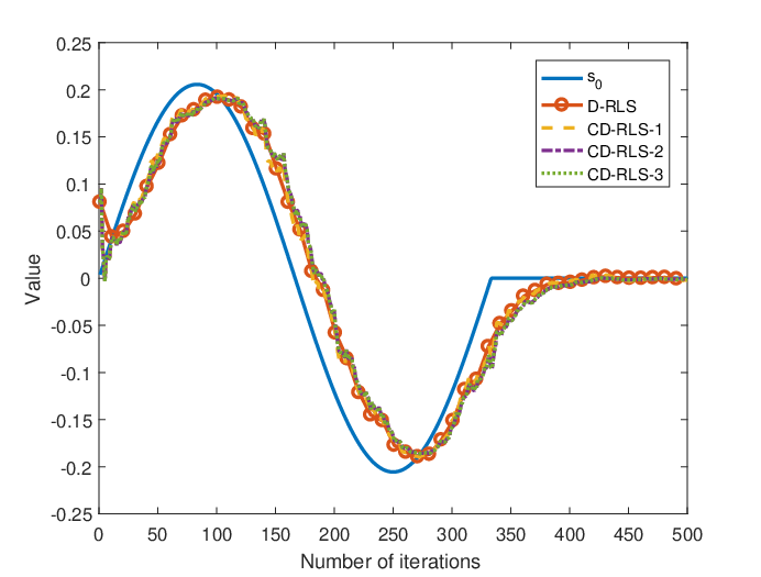
When λ<1\lambda<1, the three censoring-based strategies are also able to track time-varying signals well. Note that to track the signal dynamics in this case, the censoring ratio cannot be too large. We use the same setting of the synthetic data but change the true 𝐬0{\mathbf{s}}_{0} such that its iith element is β~i​sin⁡(3​π​t/500)\tilde{\beta}_{i}\sin(3\pi t/500) when t≤1000/3t\leq 1000/3, and remains constant after t=1000/3t=1000/3. The magnitudes β~i\tilde{\beta}_{i} are i.i.d. and follow 𝒰⁡(0,1)\mathcal{U}(0,1). The parameters of the four decentralized algorithms are the same as those in the previous synthetic experiments, except that the censoring ratio is 0.30.3 when the censoring strategies are applied. Fig. 9 depicts the evolution of the first entries in the vector estimates of the four algorithms. They show similar tracking performance, but the censoring-based algorithms incur lower communication and computation costs over D-RLS.

V Concluding Remarks

This paper introduced three data-adaptive censoring strategies that significantly reduce the computation and communication costs of the RLS algorithm over large-scale networks. The basic idea behind these strategies is to avoid inefficient computation and communication when the local observations and/or the neighboring messages are not informative. We proved convergence of the resulting algorithms in the mean-square deviation sense. Numerical experiments validated the merits of the novel schemes.

The notion of identifying and discarding less informative observations can be widely used in various large-scale online machine learning tasks including nonlinear regression, matrix completion, clustering and classification, to name a few. These constitute our future research directions.

Appendix A Equivalent Form of D-RLS

Here we prove that D-RLS recursions (2) - (5) are equivalent to (2), (6) and (7). It follows from (4) that

𝚽j​(t)​𝐬j​(t)−λ​𝚽j​(t−1)​𝐬j​(t−1)\displaystyle\mathbf{\Phi}_{j}(t){\mathbf{s}}_{j}(t)-\lambda\mathbf{\Phi}_{j}(t-1){\mathbf{s}}_{j}(t-1) (26)
=[𝝍j​(t)−12​∑j′∈𝒩j(𝐯jj′​(t−1)−𝐯j′j​(t−1))]\displaystyle=\Big[\bm{\psi}_{j}(t)-\frac{1}{2}\sum_{j^{\prime}\in\mathcal{N}_{j}}({\mathbf{v}}_{j}^{j^{\prime}}(t-1)-{\mathbf{v}}_{j^{\prime}}^{j}(t-1))\Big]
−λ⁡[𝝍j​(t−1)−12​∑j′∈𝒩j(𝐯jj′​(t−2)−𝐯j′j​(t−2))].\displaystyle-\lambda\Big[\bm{\psi}_{j}(t-1)-\frac{1}{2}\sum_{j^{\prime}\in\mathcal{N}_{j}}({\mathbf{v}}_{j}^{j^{\prime}}(t-2)-{\mathbf{v}}_{j^{\prime}}^{j}(t-2))\Big].

Applying the matrix inversion lemma to (2) yields

𝚽j​(t)=λ​𝚽j​(t−1)+𝐡j​(t)​𝐡jT​(t).\displaystyle\mathbf{\Phi}_{j}(t)=\lambda\mathbf{\Phi}_{j}(t-1)+\mathbf{h}_{j}(t)\mathbf{h}_{j}^{T}(t). (27)

Substituting 𝝍j​(t)−λ​𝝍j​(t−1)=𝐡j​(t)​xj​(t)\bm{\psi}_{j}(t)-\lambda\bm{\psi}_{j}(t-1)=\mathbf{h}_{j}(t)x_{j}(t) from (3) and λ​𝚽j​(t−1)=𝚽j​(t)−𝐡j​(t)​𝐡jT​(t)\lambda\mathbf{\Phi}_{j}(t-1)=\mathbf{\Phi}_{j}(t)-\mathbf{h}_{j}(t)\mathbf{h}_{j}^{T}(t) from (27) into (26), leads to

𝚽j​(t)​[𝐬j​(t)−𝐬j​(t−1)]=𝐡j​(t)​[xj​(t)−𝐡jT​(t)​𝐬j​(t−1)]\displaystyle\mathbf{\Phi}_{j}(t)\big[{\mathbf{s}}_{j}(t)-{\mathbf{s}}_{j}(t-1)\big]=\mathbf{h}_{j}(t)\big[x_{j}(t)-\mathbf{h}_{j}^{T}(t){\mathbf{s}}_{j}(t-1)\big]
−12∑j′∈𝒩j(𝐯jj′(t−1)−λ𝐯jj′(t−2))\displaystyle\hskip 60.00009pt-\frac{1}{2}\sum_{j^{\prime}\in\mathcal{N}_{j}}({\mathbf{v}}_{j}^{j^{\prime}}(t-1)-\lambda{\mathbf{v}}_{j}^{j^{\prime}}(t-2))
+12∑j′∈𝒩j(𝐯j′j(t−1)−λ𝐯j′j(t−2)).\displaystyle\hskip 60.00009pt+\frac{1}{2}\sum_{j^{\prime}\in\mathcal{N}_{j}}({\mathbf{v}}_{j^{\prime}}^{j}(t-1)-\lambda{\mathbf{v}}_{j^{\prime}}^{j}(t-2)). (28)

Next, we will show that if 𝜹⁡(t)\bm{\delta}(t) is defined as

𝜹⁡(t):=12​ρ​∑j′∈𝒩j(𝐯jj′​(t)−λ​𝐯jj′​(t−1))\displaystyle\bm{\delta}(t):=\frac{1}{2\rho}\sum_{j^{\prime}\in\mathcal{N}_{j}}({\mathbf{v}}_{j}^{j^{\prime}}(t)-\lambda{\mathbf{v}}_{j}^{j^{\prime}}(t-1))
−12​ρ∑j′∈𝒩j(𝐯j′j(t)−λ𝐯j′j(t−1))\displaystyle\hskip 20.00003pt-\frac{1}{2\rho}\sum_{j^{\prime}\in\mathcal{N}_{j}}({\mathbf{v}}_{j^{\prime}}^{j}(t)-\lambda{\mathbf{v}}_{j^{\prime}}^{j}(t-1)) (29)

then its update is exactly (7). This can be done by taking the difference between slots tt and t−1t-1 for (29), and substituting the update of 𝐯jj′{\mathbf{v}}_{j}^{j^{\prime}} in (5). Due to (29), it follows that (28) is equivalent to

𝚽j​(t)​[𝐬j​(t)−𝐬j​(t−1)]=𝐡j​(t)​[xj​(t)−𝐡jT​(t)​𝐬j​(t−1)]\displaystyle\mathbf{\Phi}_{j}(t)\big[{\mathbf{s}}_{j}(t)-{\mathbf{s}}_{j}(t-1)\big]=\mathbf{h}_{j}(t)\big[x_{j}(t)-\mathbf{h}_{j}^{T}(t){\mathbf{s}}_{j}(t-1)\big]
−ρ​𝜹​(t−1).\displaystyle\hskip 103.00018pt-\rho\bm{\delta}(t-1). (30)

Left multiplying (30) with 𝚽j−1​(t)\mathbf{\Phi}_{j}^{-1}(t), yields the update of 𝐬j{\mathbf{s}}_{j} in (6), and completes the proof.

Appendix B Proof of Theorem 1

Proof.

We need the following lemma in [8, Chapter 7, Theorem 4].

Lemma 1.

Let X,X1,X2,…X,X_{1},X_{2},... be random variables on some probability space. If Xn→XX_{n}\rightarrow X in probability and P​r​(|Xn|≤k)=1Pr(|X_{n}|\leq k)=1 for all nn and some kk, then Xn→XX_{n}\rightarrow X in rrth mean for all r≥1r\geq 1.

Starting with CD-RLS-1, the proof proceeds in five stages.

Stage 1. We first investigate the spectral properties of 𝚽j​(t)\mathbf{\Phi}_{j}(t) when tt is sufficiently large. Letting λ=1\lambda=1 and applying the matrix inversion lemma to the censoring form (2), we have

𝚽j​(t)=𝚽j​(t−1)+cj​(t)​𝐡j​(t)​𝐡jT​(t).\displaystyle\mathbf{\Phi}_{j}(t)=\mathbf{\Phi}_{j}(t-1)+c_{j}(t)\mathbf{h}_{j}(t)\mathbf{h}_{j}^{T}(t). (31)

Summing up from r=1r=1 to r=tr=t and using the telescopic cancellation, (31) yields

𝚽j​(t)=∑r=1tcj​(r)​𝐡j​(r)​𝐡jT​(r)+γ−1​𝐈p.\displaystyle\mathbf{\Phi}_{j}(t)=\sum_{r=1}^{t}c_{j}(r)\mathbf{h}_{j}(r)\mathbf{h}_{j}^{T}(r)+\gamma^{-1}\mathbf{I}_{p}. (32)

Thanks to the strong law of large numbers, 𝚽j​(t)/t\mathbf{\Phi}_{j}(t)/t converges to E⁡[cj​(t)​𝐡j​(t)​𝐡jT​(t)]E[c_{j}(t)\mathbf{h}_{j}(t)\mathbf{h}_{j}^{T}(t)] almost surely as t→∞t\rightarrow\infty. Observe that

E⁡[cj​(t)​𝐡j​(t)​𝐡jT​(t)]\displaystyle E[c_{j}(t)\mathbf{h}_{j}(t)\mathbf{h}_{j}^{T}(t)] (33)
=\displaystyle= E[𝐡j(t)𝐡jT(t)E[cj(t)|𝐡j(t),𝐬j(t−1)]]\displaystyle E\big[\mathbf{h}_{j}(t)\mathbf{h}_{j}^{T}(t)E[c_{j}(t)|\mathbf{h}_{j}(t),{\mathbf{s}}_{j}(t-1)]\big]
=\displaystyle= E⁡[𝐡j​(t)​𝐡jT​(t)​Pr⁡(cj​(t)=1|𝐡j​(t),𝐬j​(t−1))].\displaystyle E[\mathbf{h}_{j}(t)\mathbf{h}_{j}^{T}(t)\Pr(c_{j}(t)=1|\mathbf{h}_{j}(t),{\mathbf{s}}_{j}(t-1))].
=\displaystyle= E⁡[𝐡j​(t)​𝐡jT​(t)​(1−∫−τ+σj−1​[𝐡jT​(t)​(𝐬j​(t−1)−𝐬0)]τ+σj−1​[𝐡jT​(t)​(𝐬j​(t−1)−𝐬0)]ϕ⁡(x)​𝑑x)].\displaystyle E\left[\mathbf{h}_{j}(t)\mathbf{h}_{j}^{T}(t)\left(1-\int_{-\tau+\sigma_{j}^{-1}[\mathbf{h}_{j}^{T}(t)({\mathbf{s}}_{j}(t-1)-{\mathbf{s}}_{0})]}^{\tau+\sigma_{j}^{-1}[\mathbf{h}_{j}^{T}(t)({\mathbf{s}}_{j}(t-1)-{\mathbf{s}}_{0})]}\phi(x)dx\right)\right].

Observing the integral in (33), we know that

1>\displaystyle 1> 1−∫−τ+σj−1​[𝐡jT​(t)​(𝐬j​(t−1)−𝐬0)]τ+σj−1​[𝐡jT​(t)​(𝐬j​(t−1)−𝐬0)]ϕ⁡(x)​𝑑x\displaystyle 1-\int_{-\tau+\sigma_{j}^{-1}[\mathbf{h}_{j}^{T}(t)({\mathbf{s}}_{j}(t-1)-{\mathbf{s}}_{0})]}^{\tau+\sigma_{j}^{-1}[\mathbf{h}_{j}^{T}(t)({\mathbf{s}}_{j}(t-1)-{\mathbf{s}}_{0})]}\phi(x)dx
≥\displaystyle\geq 1−∫−ττϕ⁡(x)​𝑑x=2​Q​(τ)\displaystyle 1-\int_{-\tau}^{\tau}\phi(x)dx=2Q(\tau) (34)

where the event set that the second inequality strictly holds (namely, “≥\geq” becomes “>>”) is with nonzero measure. Thus, substituting (34) into (33) yields

E⁡[cj​(t)​𝐡j​(t)​𝐡jT​(t)]≺E⁡[𝐡j​(t)​𝐡jT​(t)]=𝐑hjE[c_{j}(t)\mathbf{h}_{j}(t)\mathbf{h}_{j}^{T}(t)]\prec E[\mathbf{h}_{j}(t)\mathbf{h}_{j}^{T}(t)]=\mathbf{R}_{h_{j}}

and

E⁡[cj​(t)​𝐡j​(t)​𝐡jT​(t)]≻2​Q​(τ)​E​[𝐡j​(t)​𝐡jT​(t)]=2​Q​(τ)​𝐑hj.E[c_{j}(t)\mathbf{h}_{j}(t)\mathbf{h}_{j}^{T}(t)]\succ 2Q(\tau)E[\mathbf{h}_{j}(t)\mathbf{h}_{j}^{T}(t)]=2Q(\tau)\mathbf{R}_{h_{j}}.

Since 𝚽j​(t)/t\mathbf{\Phi}_{j}(t)/t converges to E⁡[cj​(t)​𝐡j​(t)​𝐡jT​(t)]E[c_{j}(t)\mathbf{h}_{j}(t)\mathbf{h}_{j}^{T}(t)] almost surely as t→∞t\rightarrow\infty and 𝐡j​(t)\mathbf{h}_{j}(t) is uniformly bounded such that 𝚽j​(t)/t\mathbf{\Phi}_{j}(t)/t is also bounded (cf. (32)), we have E⁡[‖𝚽j​(t)/t‖2]E[\|\mathbf{\Phi}_{j}(t)/t\|_{2}] converges to E⁡[‖cj​(t)​𝐡j​(t)​𝐡jT​(t)‖2]E[\|c_{j}(t)\mathbf{h}_{j}(t)\mathbf{h}_{j}^{T}(t)\|_{2}] as t→∞t\rightarrow\infty by lemma 1. Therefore, 2​Q​(τ)​𝐑hj≺E⁡[cj​(t)​𝐡j​(t)​𝐡jT​(t)]≺𝐑hj2Q(\tau)\mathbf{R}_{h_{j}}\prec E[c_{j}(t)\mathbf{h}_{j}(t)\mathbf{h}_{j}^{T}(t)]\prec\mathbf{R}_{h_{j}} implies that there exists t1>0t_{1}>0, for which it holds ∀t≥t1\forall t\geq t_{1} that

2​Q​(τ)​‖𝐑hj‖2<E⁡[‖𝚽j​(t)/t‖2]<‖𝐑hj‖2\displaystyle\hskip-10.00002pt2Q(\tau)\|\mathbf{R}_{h_{j}}\|_{2}<E[\|\mathbf{\Phi}_{j}(t)/t\|_{2}]<\|\mathbf{R}_{h_{j}}\|_{2}

and consequently the expected maximum eigenvalue of 𝚽j​(t)\mathbf{\Phi}_{j}(t) satisfies

2​Q​(τ)​λmax​(𝐑hj)​t<E⁡[λmax​(𝚽j​(t))]<λmax​(𝐑hj)​t.\displaystyle\hskip-10.00002pt2Q(\tau)\lambda_{\max}(\mathbf{R}_{h_{j}})t<E[\lambda_{\max}(\mathbf{\Phi}_{j}(t))]<\lambda_{\max}(\mathbf{R}_{h_{j}})t. (35)

Observe that t​𝚽j−1​(t)t\mathbf{\Phi}^{-1}_{j}(t) converges to {E⁡[cj​(t)​𝐡j​(t)​𝐡jT​(t)]}−1\left\{E[c_{j}(t)\mathbf{h}_{j}(t)\mathbf{h}_{j}^{T}(t)]\right\}^{-1} almost surely as t→∞t\rightarrow\infty due to the convergence of 𝚽j​(t)/t\mathbf{\Phi}_{j}(t)/t to E⁡[cj​(t)​𝐡j​(t)​𝐡jT​(t)]E[c_{j}(t)\mathbf{h}_{j}(t)\mathbf{h}_{j}^{T}(t)]. Since eigenvalues of 𝚽j​(t)/t\mathbf{\Phi}_{j}(t)/t are bounded below by a positive constant when tt is large enough, there exists t2>0t_{2}>0 such that t​𝚽j−1​(t)t\mathbf{\Phi}^{-1}_{j}(t) is bounded ∀t≥t2\forall t\geq t_{2}. Following the same analysis to obtain (35), it holds ∀t≥t2\forall t\geq t_{2} that

λmax​(𝐑hj−1)/t<E⁡[λmax​(𝚽j−1​(t))]<λmax​(𝐑hj−1)/(2​Q​(τ)​t).\displaystyle\hskip-10.00002pt\lambda_{\max}(\mathbf{R}_{h_{j}}^{-1})/t<E[\lambda_{\max}(\mathbf{\Phi}^{-1}_{j}(t))]<\lambda_{\max}(\mathbf{R}_{h_{j}}^{-1})/(2Q(\tau)t). (36)

Letting t0:=max⁡(t1,t2)t_{0}:=\max(t_{1},t_{2}), (35) and (36) hold ∀t≥t0\forall t\geq t_{0}.

Stage 2. Rewrite the update of 𝐬j{\mathbf{s}}_{j} as

𝐬j​(t)\displaystyle{\mathbf{s}}_{j}(t) =𝐬j​(t−1)+cj​(t)​𝚽j−1​(t)​𝐡j​(t)​[xj​(t)−𝐡jT​(t)​𝐬j​(t−1)]\displaystyle={\mathbf{s}}_{j}(t-1)+c_{j}(t)\mathbf{\Phi}_{j}^{-1}(t)\mathbf{h}_{j}(t)\big[x_{j}(t)-\mathbf{h}_{j}^{T}(t){\mathbf{s}}_{j}(t-1)\big]
−ρ​𝚽j−1​(t)​𝜹j​(t−1).\displaystyle-\rho\mathbf{\Phi}_{j}^{-1}(t)\bm{\delta}_{j}(t-1).

Note also that for λ=1\lambda=1, the update of 𝜹j\bm{\delta}_{j} is equivalent to (cf. (18))

𝜹j​(t−1)=∑j′∈𝒩j[𝐬j​(t−1)−𝐬j′​(t−1)].\displaystyle\bm{\delta}_{j}(t-1)=\sum_{j^{\prime}\in\mathcal{N}_{j}}\big[{\mathbf{s}}_{j}(t-1)-{\mathbf{s}}_{j^{\prime}}(t-1)\big].

Letting 𝐞j​(t):=𝐬j​(t)−𝐬0\mathbf{e}_{j}(t):={\mathbf{s}}_{j}(t)-{\mathbf{s}}_{0}, the estimation error obeys the recursion

𝐞j​(t)\displaystyle\mathbf{e}_{j}(t) =𝐞j​(t−1)+cj​(t)​𝚽j−1​(t)​𝐡j​(t)​[xj​(t)−𝐡jT​(t)​𝐬j​(t−1)]\displaystyle=\mathbf{e}_{j}(t-1)+c_{j}(t)\mathbf{\Phi}_{j}^{-1}(t)\mathbf{h}_{j}(t)[x_{j}(t)-\mathbf{h}_{j}^{T}(t){\mathbf{s}}_{j}(t-1)]
−ρ𝚽j−1(t)∑j′∈𝒩j[𝐞j(t−1)−𝐞j′(t−1)].\displaystyle-\rho\mathbf{\Phi}_{j}^{-1}(t)\sum_{j^{\prime}\in\mathcal{N}_{j}}\big[\mathbf{e}_{j}(t-1)-\mathbf{e}_{j^{\prime}}(t-1)\big].

Substituting xj​(t)=𝐡j​(t)​𝐬0+ϵj​(t)x_{j}(t)=\mathbf{h}_{j}(t){\mathbf{s}}_{0}+\epsilon_{j}(t) to eliminate 𝐬j​(t−1){\mathbf{s}}_{j}(t-1), we obtain

𝐞j​(t)\displaystyle\mathbf{e}_{j}(t) =𝐞j​(t−1)−cj​(t)​𝚽j−1​(t)​𝐡j​(t)​𝐡jT​(t)​𝐞j​(t−1)\displaystyle=\mathbf{e}_{j}(t-1)-c_{j}(t)\mathbf{\Phi}_{j}^{-1}(t)\mathbf{h}_{j}(t)\mathbf{h}_{j}^{T}(t)\mathbf{e}_{j}(t-1)
+cj​(t)​𝚽j−1​(t)​𝐡j​(t)​ϵj​(t)\displaystyle+c_{j}(t)\mathbf{\Phi}_{j}^{-1}(t)\mathbf{h}_{j}(t)\epsilon_{j}(t)
−ρ𝚽j−1(t)∑j′∈𝒩j[𝐞j(t−1)−𝐞j′(t−1)].\displaystyle-\rho\mathbf{\Phi}_{j}^{-1}(t)\sum_{j^{\prime}\in\mathcal{N}_{j}}\big[\mathbf{e}_{j}(t-1)-\mathbf{e}_{j^{\prime}}(t-1)\big]. (37)

Left multiplying (37) with 𝚽j​(t)\mathbf{\Phi}_{j}(t) yields

𝚽j​(t)​𝐞j​(t)\displaystyle\mathbf{\Phi}_{j}(t)\mathbf{e}_{j}(t) (38)
=\displaystyle= 𝚽j​(t)​𝐞j​(t−1)−cj​(t)​𝐡j​(t)​𝐡jT​(t)​𝐞j​(t−1)\displaystyle\mathbf{\Phi}_{j}(t)\mathbf{e}_{j}(t-1)-c_{j}(t)\mathbf{h}_{j}(t)\mathbf{h}_{j}^{T}(t)\mathbf{e}_{j}(t-1)
+\displaystyle+ cj​(t)​𝐡j​(t)​ϵj​(t)−ρ​∑j′∈𝒩j[𝐞j​(t−1)−𝐞j′​(t−1)]\displaystyle c_{j}(t)\mathbf{h}_{j}(t)\epsilon_{j}(t)-\rho\sum_{j^{\prime}\in\mathcal{N}_{j}}\big[\mathbf{e}_{j}(t-1)-\mathbf{e}_{j^{\prime}}(t-1)\big]
=\displaystyle= 𝚽j​(t−1)​𝐞j​(t−1)\displaystyle\mathbf{\Phi}_{j}(t-1)\mathbf{e}_{j}(t-1)
+\displaystyle+ cj​(t)​𝐡j​(t)​ϵj​(t)−ρ​∑j′∈𝒩j[𝐞j​(t−1)−𝐞j′​(t−1)].\displaystyle c_{j}(t)\mathbf{h}_{j}(t)\epsilon_{j}(t)-\rho\sum_{j^{\prime}\in\mathcal{N}_{j}}\big[\mathbf{e}_{j}(t-1)-\mathbf{e}_{j^{\prime}}(t-1)\big].

Our convergence analysis result will rely on a matrix form of (38) that accounts for all nodes jj. Define vectors 𝐞⁡(t):=[𝐞1T​(t),…,𝐞JT​(t)]T∈ℝJ​p\mathbf{e}(t):=[\mathbf{e}_{1}^{T}(t),\ldots,\mathbf{e}_{J}^{T}(t)]^{T}\in\mathbb{R}^{Jp}, ϵ⁡(t):=[ϵ1T​(t),…,ϵJT​(t)]T∈ℝJ\bm{\epsilon}(t):=[\epsilon_{1}^{T}(t),\ldots,\epsilon_{J}^{T}(t)]^{T}\in\mathbb{R}^{J}, as well as block-diagonal matrices 𝚽⁡(t):=diag⁡({𝚽j​(t)})∈ℝJ​p×J​p\mathbf{\Phi}(t):=\mathrm{diag}(\{\mathbf{\Phi}_{j}(t)\})\in\mathbb{R}^{Jp\times Jp}, 𝐂⁡(t):=diag⁡({cj​(t)})∈ℝJ×J\mathbf{C}(t):=\mathrm{diag}(\{c_{j}(t)\})\in\mathbb{R}^{J\times J}, and 𝐇⁡(t):=diag⁡({𝐡j​(t)})∈ℝJ​p×J\mathbf{H}(t):=\mathrm{diag}(\{\mathbf{h}_{j}(t)\})\in\mathbb{R}^{Jp\times J}. Then (38) can be written in matrix form as

𝚽⁡(t)​𝐞​(t)\displaystyle\mathbf{\Phi}(t)\mathbf{e}(t)
=\displaystyle= [𝚽⁡(t−1)−ρ​𝐋⊗𝐈p]​𝐞​(t−1)+𝐇⁡(t)​𝐂​(t)​ϵ​(t)\displaystyle\big[\mathbf{\Phi}(t-1)-\rho\mathbf{L}\otimes\mathbf{I}_{p}\big]\mathbf{e}(t-1)+\mathbf{H}(t)\mathbf{C}(t)\bm{\epsilon}(t) (39)

which after left multiplication with 𝚽−12​(t)\mathbf{\Phi}^{-\frac{1}{2}}(t) yields

𝚽12​(t)​𝐞​(t)=\displaystyle\mathbf{\Phi}^{\frac{1}{2}}(t)\mathbf{e}(t)= 𝚽−12​(t)​[𝚽⁡(t−1)−ρ​𝐋⊗𝐈p]​𝐞​(t−1)\displaystyle\mathbf{\Phi}^{-\frac{1}{2}}(t)\big[\mathbf{\Phi}(t-1)-\rho\mathbf{L}\otimes\mathbf{I}_{p}\big]\mathbf{e}(t-1)
+\displaystyle+ 𝚽−12​(t)​𝐇​(t)​𝐂​(t)​ϵ​(t).\displaystyle\mathbf{\Phi}^{-\frac{1}{2}}(t)\mathbf{H}(t)\mathbf{C}(t)\bm{\epsilon}(t). (40)

From (40), we have (⊗\otimes denotes Kronecker product)

E⁡[𝐞T​(t)​𝚽​(t)​𝐞​(t)]\displaystyle E[\mathbf{e}^{T}(t)\mathbf{\Phi}(t)\mathbf{e}(t)]
=\displaystyle= E[𝐞T(t−1)(𝚽(t−1)−ρ𝐋⊗𝐈p)T𝚽−1(t)\displaystyle E[\mathbf{e}^{T}(t-1)(\mathbf{\Phi}(t-1)-\rho\mathbf{L}\otimes\mathbf{I}_{p})^{T}\mathbf{\Phi}^{-1}(t)
×(𝚽(t−1)−ρ𝐋⊗𝐈p)𝐞(t−1)]\displaystyle\hskip 10.00002pt\times(\mathbf{\Phi}(t-1)-\rho\mathbf{L}\otimes\mathbf{I}_{p})\mathbf{e}(t-1)]
+\displaystyle+ 2​E​[𝐞T​(t−1)​(𝚽⁡(t−1)−ρ​𝐋⊗𝐈p)T​𝚽−1​(t)​𝐇​(t)​𝐂​(t)​ϵ​(t)]\displaystyle 2E[\mathbf{e}^{T}(t-1)(\mathbf{\Phi}(t-1)-\rho\mathbf{L}\otimes\mathbf{I}_{p})^{T}\mathbf{\Phi}^{-1}(t)\mathbf{H}(t)\mathbf{C}(t)\bm{\epsilon}(t)]
+\displaystyle+ E⁡[ϵT​(t)​𝐂T​(t)​𝐇T​(t)​𝚽−1​(t)​𝐇​(t)​𝐂​(t)​ϵ​(t)].\displaystyle E[\bm{\epsilon}^{T}(t)\mathbf{C}^{T}(t)\mathbf{H}^{T}(t)\mathbf{\Phi}^{-1}(t)\mathbf{H}(t)\mathbf{C}(t)\bm{\epsilon}(t)].

Since 𝐂⁡(t)\mathbf{C}(t) and ϵ⁡(t)\bm{\epsilon}(t) are irrelevant under (as1), the second term on the right hand side is zero; hence,

E⁡[𝐞T​(t)​𝚽​(t)​𝐞​(t)]\displaystyle E[\mathbf{e}^{T}(t)\mathbf{\Phi}(t)\mathbf{e}(t)]
=\displaystyle= E[𝐞T(t−1)(𝚽(t−1)−ρ𝐋⊗𝐈p)T𝚽−1(t)\displaystyle E[\mathbf{e}^{T}(t-1)(\mathbf{\Phi}(t-1)-\rho\mathbf{L}\otimes\mathbf{I}_{p})^{T}\mathbf{\Phi}^{-1}(t)
×\displaystyle\times (𝚽(t−1)−ρ𝐋⊗𝐈p)𝐞(t−1)]\displaystyle(\mathbf{\Phi}(t-1)-\rho\mathbf{L}\otimes\mathbf{I}_{p})\mathbf{e}(t-1)]
+\displaystyle+ E⁡[ϵT​(t)​𝐂T​(t)​𝐇T​(t)​𝚽−1​(t)​𝐇​(t)​𝐂​(t)​ϵ​(t)].\displaystyle E[\bm{\epsilon}^{T}(t)\mathbf{C}^{T}(t)\mathbf{H}^{T}(t)\mathbf{\Phi}^{-1}(t)\mathbf{H}(t)\mathbf{C}(t)\bm{\epsilon}(t)]. (41)

Stage 3. Consider the first term on the right hand side of (41). Since 𝐋\mathbf{L} is positive semi-definite, we can find a matrix 𝐔=(𝐋⊗𝐈p)12\mathbf{U}=(\mathbf{L}\otimes\mathbf{I}_{p})^{\frac{1}{2}} such that 𝐋⊗𝐈p=𝐔T​𝐔\mathbf{L}\otimes\mathbf{I}_{p}=\mathbf{U}^{T}\mathbf{U}. By the matrix inversion lemma, it holds that

(𝚽⁡(t−1)−ρ​𝐋⊗𝐈p)−1\displaystyle(\mathbf{\Phi}(t-1)-\rho\mathbf{L}\otimes\mathbf{I}_{p})^{-1}
=\displaystyle= (𝚽⁡(t−1)−ρ​𝐔T​𝐔)−1\displaystyle(\mathbf{\Phi}(t-1)-\rho\mathbf{U}^{T}\mathbf{U})^{-1}
=\displaystyle= 𝚽−1​(t−1)+ρ​𝚽−1​(t−1)​𝐔T\displaystyle\mathbf{\Phi}^{-1}(t-1)+\rho\mathbf{\Phi}^{-1}(t-1)\mathbf{U}^{T}
×\displaystyle\times (𝐈J​p−ρ​𝐔​𝚽−1​(t−1)​𝐔T)−1​𝐔​𝚽−1​(t−1).\displaystyle(\mathbf{I}_{Jp}-\rho\mathbf{U}\mathbf{\Phi}^{-1}(t-1)\mathbf{U}^{T})^{-1}\mathbf{U}\mathbf{\Phi}^{-1}(t-1). (42)

For λ=1\lambda=1, it follows from (2) that 𝚽−1​(t−1)−𝚽−1​(t)⪰𝟎J​p\mathbf{\Phi}^{-1}(t-1)-\mathbf{\Phi}^{-1}(t)\succeq\mathbf{0}_{Jp}. Since 𝚽−1​(0)=γ​𝐈J​p\mathbf{\Phi}^{-1}(0)=\gamma\mathbf{I}_{Jp}, it holds that 𝚽−1​(t−1)⪯γ​𝐈J​p\mathbf{\Phi}^{-1}(t-1)\preceq\gamma\mathbf{I}_{Jp} for all t≥1t\geq 1, and consequently

𝐈J​p−ρ​𝐔​𝚽−1​(t−1)​𝐔T⪰𝐈J​p−ρ​γ​𝐔𝐔T=𝐈J​p−ρ​γ​𝐋⊗𝐈p.\displaystyle\hskip-5.0pt\mathbf{I}_{Jp}-\rho\mathbf{U}\mathbf{\Phi}^{-1}(t-1)\mathbf{U}^{T}\succeq\mathbf{I}_{Jp}-\rho\gamma\mathbf{U}\mathbf{U}^{T}=\mathbf{I}_{Jp}-\rho\gamma\mathbf{L}\otimes\mathbf{I}_{p}.

If 0<ρ<1/(γ​λmax​(𝐋))0<\rho<1/(\gamma\lambda_{\max}(\mathbf{L})), then for all t≥1t\geq 1 it follows that

𝐈J​p−ρ​𝐔​𝚽−1​(t−1)​𝐔T⪰𝟎J​p.\displaystyle\mathbf{I}_{Jp}-\rho\mathbf{U}\mathbf{\Phi}^{-1}(t-1)\mathbf{U}^{T}\succeq\mathbf{0}_{Jp}.

This implies that the second term of (42) is positive definite. Thus, we have

𝚽−1​(t)⪯𝚽−1​(t−1)⪯(𝚽⁡(t−1)−ρ​𝐋⊗𝐈p)−1\displaystyle\mathbf{\Phi}^{-1}(t)\preceq\mathbf{\Phi}^{-1}(t-1)\preceq(\mathbf{\Phi}(t-1)-\rho\mathbf{L}\otimes\mathbf{I}_{p})^{-1} (43)

and hence, the first term on the right hand side of (41) is bounded by

E[𝐞T(t−1)(𝚽(t−1)−ρ𝐋⊗𝐈p)T𝚽−1(t)\displaystyle E[\mathbf{e}^{T}(t-1)(\mathbf{\Phi}(t-1)-\rho\mathbf{L}\otimes\mathbf{I}_{p})^{T}\mathbf{\Phi}^{-1}(t)
×(𝚽(t−1)−ρ𝐋⊗𝐈p)𝐞(t−1)]\displaystyle\hskip 10.00002pt\times(\mathbf{\Phi}(t-1)-\rho\mathbf{L}\otimes\mathbf{I}_{p})\mathbf{e}(t-1)]
≤\displaystyle\leq E⁡[𝐞T​(t−1)​(𝚽⁡(t−1)−ρ​𝐋⊗𝐈p)T​𝐞​(t−1)]\displaystyle E[\mathbf{e}^{T}(t-1)(\mathbf{\Phi}(t-1)-\rho\mathbf{L}\otimes\mathbf{I}_{p})^{T}\mathbf{e}(t-1)]
≤\displaystyle\leq E⁡[𝐞T​(t−1)​𝚽​(t−1)T​𝐞​(t−1)].\displaystyle E[\mathbf{e}^{T}(t-1)\mathbf{\Phi}(t-1)^{T}\mathbf{e}(t-1)]. (44)

Stage 4. Now consider the second term on the right hand side of (41). Manipulating the expectation yields

E⁡[ϵT​(t)​𝐂T​(t)​𝐇T​(t)​𝚽−1​(t)​𝐇​(t)​𝐂​(t)​ϵ​(t)]\displaystyle E[\bm{\epsilon}^{T}(t)\mathbf{C}^{T}(t)\mathbf{H}^{T}(t)\mathbf{\Phi}^{-1}(t)\mathbf{H}(t)\mathbf{C}(t)\bm{\epsilon}(t)]
=\displaystyle= E⁡[tr⁡(ϵT​(t)​𝐂T​(t)​𝐇T​(t)​𝚽−1​(t)​𝐇​(t)​𝐂​(t)​ϵ​(t))]\displaystyle E[\mathrm{tr}(\bm{\epsilon}^{T}(t)\mathbf{C}^{T}(t)\mathbf{H}^{T}(t)\mathbf{\Phi}^{-1}(t)\mathbf{H}(t)\mathbf{C}(t)\bm{\epsilon}(t))]
=\displaystyle= E⁡[tr⁡(𝐂T​(t)​𝐇T​(t)​𝚽−1​(t)​𝐇​(t)​𝐂​(t)​ϵ​(t)​ϵT​(t))]\displaystyle E[\mathrm{tr}(\mathbf{C}^{T}(t)\mathbf{H}^{T}(t)\mathbf{\Phi}^{-1}(t)\mathbf{H}(t)\mathbf{C}(t)\bm{\epsilon}(t)\bm{\epsilon}^{T}(t))]
=\displaystyle= E[tr(𝐂T(t)𝐇T(t)𝚽−1(t)𝐇(t)𝐂(t)diag({σj2})].\displaystyle E[\mathrm{tr}(\mathbf{C}^{T}(t)\mathbf{H}^{T}(t)\mathbf{\Phi}^{-1}(t)\mathbf{H}(t)\mathbf{C}(t)\mathrm{diag}(\{\sigma_{j}^{2}\})].

where diag⁡({σj2})∈ℝJ×J\mathrm{diag}(\{\sigma_{j}^{2}\})\in\mathbb{R}^{J\times J} is a diagonal matrix constructed with {σj2}j=1J\{\sigma_{j}^{2}\}_{j=1}^{J} on its diagonal. Expanding the matrix multiplications and noting that cj​(t)≤1c_{j}(t)\leq 1, we obtain

E⁡[ϵT​(t)​𝐂T​(t)​𝐇T​(t)​𝚽−1​(t)​𝐇​(t)​𝐂​(t)​ϵ​(t)]\displaystyle E[\bm{\epsilon}^{T}(t)\mathbf{C}^{T}(t)\mathbf{H}^{T}(t)\mathbf{\Phi}^{-1}(t)\mathbf{H}(t)\mathbf{C}(t)\bm{\epsilon}(t)]
≤\displaystyle\leq ∑j=1Jσj2​E​[𝐡jT​(t)​𝚽j−1​(t)​𝐡j​(t)].\displaystyle\sum_{j=1}^{J}\sigma_{j}^{2}E[\mathbf{h}_{j}^{T}(t)\mathbf{\Phi}_{j}^{-1}(t)\mathbf{h}_{j}(t)].

Because 𝚽j−1​(t−1)⪰𝚽j−1​(t)\mathbf{\Phi}_{j}^{-1}(t-1)\succeq\mathbf{\Phi}_{j}^{-1}(t) due to (22), we further have

E⁡[ϵT​(t)​𝐂T​(t)​𝐇T​(t)​𝚽−1​(t)​𝐇​(t)​𝐂​(t)​ϵ​(t)]\displaystyle E[\bm{\epsilon}^{T}(t)\mathbf{C}^{T}(t)\mathbf{H}^{T}(t)\mathbf{\Phi}^{-1}(t)\mathbf{H}(t)\mathbf{C}(t)\bm{\epsilon}(t)]
≤\displaystyle\leq ∑j=1Jσj2​E​[𝐡jT​(t)​𝚽j−1​(t−1)​𝐡j​(t)]\displaystyle\sum_{j=1}^{J}\sigma_{j}^{2}E[\mathbf{h}_{j}^{T}(t)\mathbf{\Phi}_{j}^{-1}(t-1)\mathbf{h}_{j}(t)]
≤\displaystyle\leq ∑j=1Jσj2​E​[λmax​(𝚽j−1​(t−1))​‖𝐡j​(t)‖2].\displaystyle\sum_{j=1}^{J}\sigma_{j}^{2}E[\lambda_{\max}(\mathbf{\Phi}_{j}^{-1}(t-1))\|\mathbf{h}_{j}(t)\|^{2}]. (45)

Since 𝚽j−1​(t−1)\mathbf{\Phi}_{j}^{-1}(t-1) and 𝐡j​(t)\mathbf{h}_{j}(t) are independent, it holds ∀t>t0\forall t>t_{0} that

E⁡[λmax​(𝚽j−1​(t−1))​‖𝐡j​(t)‖2]\displaystyle E[\lambda_{\max}(\mathbf{\Phi}_{j}^{-1}(t-1))\|\mathbf{h}_{j}(t)\|^{2}]
=\displaystyle= E⁡[λmax​(𝚽j−1​(t−1))]​E​[‖𝐡j​(t)‖2]\displaystyle E[\lambda_{\max}(\mathbf{\Phi}_{j}^{-1}(t-1))]E[\|\mathbf{h}_{j}(t)\|^{2}]
<\displaystyle< λmax​(𝐑hj−1)2​Q​(τ)​(t−1)​tr​(𝐑hj).\displaystyle\frac{\lambda_{\max}(\mathbf{R}_{h_{j}}^{-1})}{2Q(\tau)(t-1)}\mathrm{tr}(\mathbf{R}_{h_{j}}). (46)

The inequality is due to (36) that shows E⁡[λmax​(𝚽j−1​(t))]<λmax​(𝐑hj−1)/(2​Q​(τ)​t)E[\lambda_{\max}(\mathbf{\Phi}^{-1}_{j}(t))]<\lambda_{\max}(\mathbf{R}_{h_{j}}^{-1})/(2Q(\tau)t), ∀t≥t0\forall t\geq t_{0} and the fact E⁡[‖𝐡j​(t)‖2]=tr⁡(E⁡[𝐡j​(t)​𝐡jT​(t)])=tr⁡(𝐑hj)E[\|\mathbf{h}_{j}(t)\|^{2}]=\mathrm{tr}(E[\mathbf{h}_{j}(t)\mathbf{h}_{j}^{T}(t)])=\mathrm{tr}(\mathbf{R}_{h_{j}}). Using (46) allows one to deduce from (45) that

E⁡[ϵT​(t)​𝐂T​(t)​𝐇T​(t)​𝚽−1​(t)​𝐇​(t)​𝐂​(t)​ϵ​(t)]\displaystyle E[\bm{\epsilon}^{T}(t)\mathbf{C}^{T}(t)\mathbf{H}^{T}(t)\mathbf{\Phi}^{-1}(t)\mathbf{H}(t)\mathbf{C}(t)\bm{\epsilon}(t)]
≤\displaystyle\leq 12​Q​(τ)​(t−1)​∑j=1Jσj2​λmax​(𝐑hj−1)​tr​(𝐑hj)\displaystyle\frac{1}{2Q(\tau)(t-1)}\sum_{j=1}^{J}\sigma_{j}^{2}\lambda_{\max}(\mathbf{R}_{h_{j}}^{-1})\mathrm{tr}(\mathbf{R}_{h_{j}}) (47)

holds ∀t>t0\forall t>t_{0}.

For t≤t0t\leq t_{0}, we have 𝚽j−1​(t)⪯𝚽j−1​(0)=γ​𝐈p\mathbf{\Phi}_{j}^{-1}(t)\preceq\mathbf{\Phi}_{j}^{-1}(0)=\gamma\mathbf{I}_{p} because to (43), and thus

∑j=1Jσj2​E​[𝐡jT​(t)​𝚽j−1​(t)​𝐡j​(t)]\displaystyle\sum_{j=1}^{J}\sigma_{j}^{2}E[\mathbf{h}_{j}^{T}(t)\mathbf{\Phi}_{j}^{-1}(t)\mathbf{h}_{j}(t)]
≤\displaystyle\leq ∑j=1Jγ​σj2​E​[𝐡jT​(t)​𝐡j​(t)]=γ​∑j=1Jσj2​t​r​(𝐑hj).\displaystyle\sum_{j=1}^{J}\gamma\sigma_{j}^{2}E[\mathbf{h}_{j}^{T}(t)\mathbf{h}_{j}(t)]=\gamma\sum_{j=1}^{J}\sigma_{j}^{2}tr(\mathbf{R}_{h_{j}}).

Therefore, for t≤t0t\leq t_{0} (45) yields

E⁡[ϵT​(t)​𝐂T​(t)​𝐇T​(t)​𝚽−1​(t)​𝐇​(t)​𝐂​(t)​ϵ​(t)]\displaystyle E[\bm{\epsilon}^{T}(t)\mathbf{C}^{T}(t)\mathbf{H}^{T}(t)\mathbf{\Phi}^{-1}(t)\mathbf{H}(t)\mathbf{C}(t)\bm{\epsilon}(t)]
≤\displaystyle\leq γ​∑j=1Jσj2​tr​(𝐑hj).\displaystyle\gamma\sum_{j=1}^{J}\sigma_{j}^{2}\mathrm{tr}(\mathbf{R}_{h_{j}}). (48)

Stage 5. Substituting (44), (47) and (48) into (41) implies for t>t0t>t_{0} that

E⁡[𝐞T​(t)​𝚽​(t)​𝐞​(t)]\displaystyle E[\mathbf{e}^{T}(t)\mathbf{\Phi}(t)\mathbf{e}(t)]
≤\displaystyle\leq E⁡[𝐞T​(t−1)​𝚽​(t−1)​𝐞​(t−1)]\displaystyle E[\mathbf{e}^{T}(t-1)\mathbf{\Phi}(t-1)\mathbf{e}(t-1)]
+\displaystyle+ 12​Q​(τ)​(t−1)​∑j=1Jσj2​λmax​(𝐑hj−1)​tr​(𝐑hj)\displaystyle\frac{1}{2Q(\tau)(t-1)}\sum_{j=1}^{J}\sigma_{j}^{2}\lambda_{\max}(\mathbf{R}_{h_{j}}^{-1})\mathrm{tr}(\mathbf{R}_{h_{j}}) (49)

while for t≤t0t\leq t_{0}

E⁡[𝐞T​(t)​𝚽​(t)​𝐞​(t)]\displaystyle E[\mathbf{e}^{T}(t)\mathbf{\Phi}(t)\mathbf{e}(t)]
≤\displaystyle\leq E⁡[𝐞T​(t−1)​𝚽​(t−1)​𝐞​(t−1)]+γ​∑j=1Jσj2​tr​(𝐑hj).\displaystyle E[\mathbf{e}^{T}(t-1)\mathbf{\Phi}(t-1)\mathbf{e}(t-1)]+\gamma\sum_{j=1}^{J}\sigma_{j}^{2}\mathrm{tr}(\mathbf{R}_{h_{j}}). (50)

Summing (49) from r=t0+1r=t_{0}+1 to r=tr=t and (50) from r=1r=1 to r=t0r=t_{0}, applying telescopic cancellation, and noticing that 𝚽⁡(0)=γ−1​𝐈J​p\mathbf{\Phi}(0)=\gamma^{-1}\mathbf{I}_{Jp}, yields for t>t0t>t_{0}

E⁡[𝐞T​(t)​𝚽​(t)​𝐞​(t)]\displaystyle E[\mathbf{e}^{T}(t)\mathbf{\Phi}(t)\mathbf{e}(t)] (51)
≤\displaystyle\leq γ−1​‖𝐞⁡(0)‖2+(γ​t0+∑r=t0+1tλmax​(𝐑hj−1)2​Q​(τ)​(t−1))​∑j=1Jσj2​tr​(𝐑hj)\displaystyle\gamma^{-1}||\mathbf{e}(0)||^{2}+(\gamma t_{0}+\sum_{r=t_{0}+1}^{t}\frac{\lambda_{\max}(\mathbf{R}_{h_{j}}^{-1})}{2Q(\tau)(t-1)})\sum_{j=1}^{J}\sigma_{j}^{2}\mathrm{tr}(\mathbf{R}_{h_{j}})
≤\displaystyle\leq γ−1​‖𝐞⁡(0)‖2+(γ​t0+λmax​(𝐑hj−1)2​Q​(τ)​ln⁡(t))​∑j=1Jσj2​tr​(𝐑hj).\displaystyle\gamma^{-1}||\mathbf{e}(0)||^{2}+(\gamma t_{0}+\frac{\lambda_{\max}(\mathbf{R}_{h_{j}}^{-1})}{2Q(\tau)}\ln(t))\sum_{j=1}^{J}\sigma_{j}^{2}\mathrm{tr}(\mathbf{R}_{h_{j}}).

On the other hand, it holds

E⁡[𝐞T​(t)​𝚽​(t)​𝐞​(t)]\displaystyle E[\mathbf{e}^{T}(t)\mathbf{\Phi}(t)\mathbf{e}(t)] ≥E⁡[‖𝐞⁡(t)‖2/λmax​(𝚽−1​(t))]\displaystyle\geq E[\|\mathbf{e}(t)\|^{2}/\lambda_{\max}(\mathbf{\Phi}^{-1}(t))]
≥E​[‖𝐞⁡(t)‖]2/E⁡[λmax​(𝚽−1​(t))]\displaystyle\geq E[\|\mathbf{e}(t)\|]^{2}/E[\lambda_{\max}(\mathbf{\Phi}^{-1}(t))]

where the last line is due to Cauchy-Schwarz inequality

E⁡[‖𝐞⁡(t)‖2/λmax​(𝚽−1​(t))]​E​[λmax​(𝚽−1​(t))]\displaystyle E[\|\mathbf{e}(t)\|^{2}/\lambda_{\max}(\mathbf{\Phi}^{-1}(t))]E[\lambda_{\max}(\mathbf{\Phi}^{-1}(t))]
=\displaystyle= E⁡[(‖𝐞⁡(t)‖/λmax​(𝚽−1​(t))12)2]​E​[(λmax​(𝚽−1​(t))12)2]\displaystyle E[\left(\|\mathbf{e}(t)\|/\lambda_{\max}(\mathbf{\Phi}^{-1}(t))^{\frac{1}{2}}\right)^{2}]E[\left(\lambda_{\max}(\mathbf{\Phi}^{-1}(t))^{\frac{1}{2}}\right)^{2}]
≥\displaystyle\geq E​[‖𝐞⁡(t)‖]2.\displaystyle E[\|\mathbf{e}(t)\|]^{2}.

From (36), E⁡[λmax​(𝚽j−1​(t))]<λmax​(𝐑hj−1)/(2​Q​(τ)​t)=1/(λmin​(𝐑hj)​2​Q​(τ)​t)E[\lambda_{\max}(\mathbf{\Phi}^{-1}_{j}(t))]<\lambda_{\max}(\mathbf{R}_{h_{j}}^{-1})/(2Q(\tau)t)=1/(\lambda_{\min}(\mathbf{R}_{h_{j}})2Q(\tau)t) holds asymptotically. Definining μ:=min⁡{λmin​(𝐑hj),j∈𝒱}\mu:=\min\{\lambda_{\min}(\mathbf{R}_{h_{j}}),j\in\mathcal{V}\}, we establish that

2​Q​(τ)​μ​t​E​[‖𝐞⁡(t)‖2]≤E⁡[𝐞T​(t)​𝚽​(t)​𝐞​(t)],t>t0.\displaystyle 2Q(\tau)\mu tE[||\mathbf{e}(t)||^{2}]\leq E[\mathbf{e}^{T}(t)\mathbf{\Phi}(t)\mathbf{e}(t)],\quad t>t_{0}. (52)

Combining (51) and (52) implies

2​Q​(τ)​μ​t​E​[‖𝐞⁡(t)‖]2\displaystyle 2Q(\tau)\mu tE[||\mathbf{e}(t)||]^{2} (53)
≤\displaystyle\leq γ−1​‖𝐞⁡(0)‖2+(γ​t0+λmax​(𝐑hj−1)2​Q​(τ)​ln⁡(t))​∑j=1Jσj2​tr​(𝐑hj).\displaystyle\gamma^{-1}||\mathbf{e}(0)||^{2}+(\gamma t_{0}+\frac{\lambda_{\max}(\mathbf{R}_{h_{j}}^{-1})}{2Q(\tau)}\ln(t))\sum_{j=1}^{J}\sigma_{j}^{2}\mathrm{tr}(\mathbf{R}_{h_{j}}).

Finally, with ‖𝐞⁡(t)‖2:=∑j=1J‖𝐞j​(t)‖2=∑j=1J‖𝐬j​(t)−𝐬0‖2||\mathbf{e}(t)||^{2}:=\sum_{j=1}^{J}||\mathbf{e}_{j}(t)||^{2}=\sum_{j=1}^{J}||{\mathbf{s}}_{j}(t)-{\mathbf{s}}_{0}||^{2} this leads to (24), which completes the proof of CD-RLS-1.

Consider next CD-RLS-2. Stage 1 of the proof remains the same, while for Stage 2, 𝐞j​(t−1)−𝐞j′​(t−1)\mathbf{e}_{j}(t-1)-\mathbf{e}_{j^{\prime}}(t-1) is replaced by cj​(t)​[𝐞j​(t−1)−𝐞j′​(t−1)]c_{j}(t)\big[\mathbf{e}_{j}(t-1)-\mathbf{e}_{j^{\prime}}(t-1)\big] in (38) to arrive at

𝚽j​(t)​𝐞j​(t)\displaystyle\mathbf{\Phi}_{j}(t)\mathbf{e}_{j}(t) (54)
=\displaystyle= 𝚽j​(t−1)​𝐞j​(t−1)−cj​(t)​𝐡j​(t)​𝐡jT​(t)​𝐞j​(t−1)\displaystyle\mathbf{\Phi}_{j}(t-1)\mathbf{e}_{j}(t-1)-c_{j}(t)\mathbf{h}_{j}(t)\mathbf{h}_{j}^{T}(t)\mathbf{e}_{j}(t-1)
+\displaystyle+ cj​(t)​𝐡j​(t)​ϵj​(t)−ρ​∑j′∈𝒩jcj​(t)​[𝐞j​(t−1)−𝐞j′​(t−1)].\displaystyle c_{j}(t)\mathbf{h}_{j}(t)\epsilon_{j}(t)-\rho\sum_{j^{\prime}\in\mathcal{N}_{j}}c_{j}(t)\big[\mathbf{e}_{j}(t-1)-\mathbf{e}_{j^{\prime}}(t-1)\big].

Its matrix form (41) can be expressed as

E⁡[𝐞T​(t)​𝚽​(t)​𝐞​(t)]\displaystyle E[\mathbf{e}^{T}(t)\mathbf{\Phi}(t)\mathbf{e}(t)]
=\displaystyle= E[𝐞T(t−1)(𝚽(t−1)−ρ(𝐂(t)𝐋)⊗𝐈p)T𝚽−1(t)\displaystyle E[\mathbf{e}^{T}(t-1)(\mathbf{\Phi}(t-1)-\rho(\mathbf{C}(t)\mathbf{L})\otimes\mathbf{I}_{p})^{T}\mathbf{\Phi}^{-1}(t)
×(𝚽(t−1)−ρ(𝐂(t)𝐋)⊗𝐈p)𝐞(t−1)]\displaystyle\hskip 10.00002pt\times(\mathbf{\Phi}(t-1)-\rho(\mathbf{C}(t)\mathbf{L})\otimes\mathbf{I}_{p})\mathbf{e}(t-1)]
+\displaystyle+ E⁡[ϵT​(t)​𝐂T​(t)​𝐇T​(t)​𝚽−1​(t)​𝐇​(t)​𝐂​(t)​ϵ​(t)].\displaystyle E[\bm{\epsilon}^{T}(t)\mathbf{C}^{T}(t)\mathbf{H}^{T}(t)\mathbf{\Phi}^{-1}(t)\mathbf{H}(t)\mathbf{C}(t)\bm{\epsilon}(t)]. (55)

Observe that the right hand sides of (41) and (55) are only different in their first terms. Similar to Stage 3 (cf. (44)), we need to show that the first term satisfies

E[𝐞T(t−1)(𝚽(t−1)−ρ(𝐂(t)𝐋)⊗𝐈p)T𝚽−1(t)\displaystyle E[\mathbf{e}^{T}(t-1)(\mathbf{\Phi}(t-1)-\rho(\mathbf{C}(t)\mathbf{L})\otimes\mathbf{I}_{p})^{T}\mathbf{\Phi}^{-1}(t)
×(𝚽(t−1)−ρ(𝐂(t)𝐋)⊗𝐈p)𝐞(t−1)]\displaystyle\hskip 10.00002pt\times(\mathbf{\Phi}(t-1)-\rho(\mathbf{C}(t)\mathbf{L})\otimes\mathbf{I}_{p})\mathbf{e}(t-1)]
≤\displaystyle\leq E⁡[𝐞T​(t−1)​𝚽​(t−1)​𝐞​(t−1)].\displaystyle E[\mathbf{e}^{T}(t-1)\mathbf{\Phi}(t-1)\mathbf{e}(t-1)]. (56)

Substituting the update (22) with λ=1\lambda=1 into (56), it suffices to prove that

E[𝐞T(t−1)𝐂(t)⊗𝐈p𝐇(t)𝐇T(t)\displaystyle E[\mathbf{e}^{T}(t-1)\mathbf{C}(t)\otimes\mathbf{I}_{p}\mathbf{H}(t)\mathbf{H}^{T}(t) (57)
×(𝐈J+𝐇T(t)𝚽−1(t−1)𝐇(t))−1⊗𝐈p𝐞(t−1)]\displaystyle\hskip 10.00002pt\times(\mathbf{I}_{J}+\mathbf{H}^{T}(t)\mathbf{\Phi}^{-1}(t-1)\mathbf{H}(t))^{-1}\otimes\mathbf{I}_{p}\mathbf{e}(t-1)]
≥\displaystyle\geq ρ​E​[𝐞T​(t−1)​𝐖𝐞​(t−1)]\displaystyle\rho E[\mathbf{e}^{T}(t-1)\mathbf{W}\mathbf{e}(t-1)]

where

𝐖:=\displaystyle\mathbf{W}:= 𝐖1+𝐖1T−𝐖2−(𝐋𝐂⁡(t))⊗𝐈p−(𝐂⁡(t)​𝐋)⊗𝐈p\displaystyle\mathbf{W}_{1}+\mathbf{W}_{1}^{T}-\mathbf{W}_{2}-(\mathbf{L}\mathbf{C}(t))\otimes\mathbf{I}_{p}-(\mathbf{C}(t)\mathbf{L})\otimes\mathbf{I}_{p}
+\displaystyle+ ρ​𝐋⊗𝐈p​𝚽−1​(t−1)​(𝐂⁡(t)​𝐋)⊗𝐈p\displaystyle\rho\mathbf{L}\otimes\mathbf{I}_{p}\mathbf{\Phi}^{-1}(t-1)(\mathbf{C}(t)\mathbf{L})\otimes\mathbf{I}_{p}
𝐖1:=\displaystyle\mathbf{W}_{1}:= 𝐂⁡(t)⊗𝐈p​𝐇​(t)​𝐇T​(t)​𝚽−1​(t−1)\displaystyle\mathbf{C}(t)\otimes\mathbf{I}_{p}\mathbf{H}(t)\mathbf{H}^{T}(t)\mathbf{\Phi}^{-1}(t-1)
×\displaystyle\times ((𝐈J+𝐇T​(t)​𝚽−1​(t−1)​𝐇​(t))−1​𝐋)⊗𝐈p\displaystyle((\mathbf{I}_{J}+\mathbf{H}^{T}(t)\mathbf{\Phi}^{-1}(t-1)\mathbf{H}(t))^{-1}\mathbf{L})\otimes\mathbf{I}_{p}
𝐖2:=\displaystyle\mathbf{W}_{2}:= (𝐋𝐂⁡(t))⊗𝐈p​𝚽−1​(t−1)​𝐇​(t)​𝐇T​(t)​𝚽−1​(t−1)\displaystyle(\mathbf{L}\mathbf{C}(t))\otimes\mathbf{I}_{p}\mathbf{\Phi}^{-1}(t-1)\mathbf{H}(t)\mathbf{H}^{T}(t)\mathbf{\Phi}^{-1}(t-1)
×\displaystyle\times ((𝐈J+𝐇T​(t)​𝚽−1​(t−1)​𝐇​(t))−1​𝐋)⊗𝐈p.\displaystyle((\mathbf{I}_{J}+\mathbf{H}^{T}(t)\mathbf{\Phi}^{-1}(t-1)\mathbf{H}(t))^{-1}\mathbf{L})\otimes\mathbf{I}_{p}.

For the left hand side of (57), use the lower bound of the conditional expectation 2Q(τ)≤E[cj(t)|𝐡j(t),𝐬j(t−1)]2Q(\tau)\leq E[c_{j}(t)|\mathbf{h}_{j}(t),{\mathbf{s}}_{j}(t-1)] to eliminate 𝐂⁡(t)\mathbf{C}(t), and arrive at

E[𝐞T(t−1)𝐂(t)⊗𝐈p𝐇(t)𝐇T(t)\displaystyle E[\mathbf{e}^{T}(t-1)\mathbf{C}(t)\otimes\mathbf{I}_{p}\mathbf{H}(t)\mathbf{H}^{T}(t) (58)
×(𝐈J+𝐇T(t)𝚽−1(t−1)𝐇(t))−1⊗𝐈p𝐞(t−1)]\displaystyle\hskip 10.00002pt\times(\mathbf{I}_{J}+\mathbf{H}^{T}(t)\mathbf{\Phi}^{-1}(t-1)\mathbf{H}(t))^{-1}\otimes\mathbf{I}_{p}\mathbf{e}(t-1)]
≥\displaystyle\geq 2Q(τ)E[𝐞T(t−1)𝐇(t)𝐇T(t)\displaystyle 2Q(\tau)E[\mathbf{e}^{T}(t-1)\mathbf{H}(t)\mathbf{H}^{T}(t)
×(𝐈J+𝐇T(t)𝚽−1(t−1)𝐇(t))−1⊗𝐈p𝐞(t−1)].\displaystyle\hskip 10.00002pt\times(\mathbf{I}_{J}+\mathbf{H}^{T}(t)\mathbf{\Phi}^{-1}(t-1)\mathbf{H}(t))^{-1}\otimes\mathbf{I}_{p}\mathbf{e}(t-1)].

By (43), it holds that 𝚽−1​(t−1)⪯𝚽−1​(0)=γ​𝐈J​p\mathbf{\Phi}^{-1}(t-1)\preceq\mathbf{\Phi}^{-1}(0)=\gamma\mathbf{I}_{Jp}, and thus

[𝐈J+𝐇T​(t)​𝚽−1​(t−1)​𝐇​(t)]−1⪰[𝐈J+γ​𝐇T​(t)​𝐇​(t)]−1.\displaystyle\left[\mathbf{I}_{J}+\mathbf{H}^{T}(t)\mathbf{\Phi}^{-1}(t-1)\mathbf{H}(t)\right]^{-1}\succeq\left[\mathbf{I}_{J}+\gamma\mathbf{H}^{T}(t)\mathbf{H}(t)\right]^{-1}.

By assumption {𝐡j​(t)}\{{\bf h}_{j}(t)\} are uniformly bounded. If 𝐡jT​(t)​𝐡j​(t)≤K{\bf h}_{j}^{T}(t){\bf h}_{j}(t)\leq K for all j=1,…,Jj=1,\ldots,J, we find

[𝐈J+𝐇T​(t)​𝚽−1​(t−1)​𝐇​(t)]−1⪰11+γ​K2​𝐈J.\displaystyle\left[\mathbf{I}_{J}+\mathbf{H}^{T}(t)\mathbf{\Phi}^{-1}(t-1)\mathbf{H}(t)\right]^{-1}\succeq\frac{1}{1+\gamma K^{2}}\mathbf{I}_{J}. (59)

Substituting (59) into (58), we obtain a lower bound for the left hand side of (57) given by

E[𝐞T(t−1)𝐂(t)⊗𝐈p𝐇(t)𝐇T(t)\displaystyle E[\mathbf{e}^{T}(t-1)\mathbf{C}(t)\otimes\mathbf{I}_{p}\mathbf{H}(t)\mathbf{H}^{T}(t) (60)
×(𝐈J+𝐇T(t)𝚽−1(t−1)𝐇(t))−1⊗𝐈p𝐞(t−1)]\displaystyle\hskip 10.00002pt\times(\mathbf{I}_{J}+\mathbf{H}^{T}(t)\mathbf{\Phi}^{-1}(t-1)\mathbf{H}(t))^{-1}\otimes\mathbf{I}_{p}\mathbf{e}(t-1)]
≥\displaystyle\geq 2​Q​(τ)1+γ​K2​E​[𝐞T​(t−1)​𝐇​(t)​𝐇T​(t)​𝐞​(t−1)]\displaystyle\frac{2Q(\tau)}{1+\gamma K^{2}}E[\mathbf{e}^{T}(t-1)\mathbf{H}(t)\mathbf{H}^{T}(t)\mathbf{e}(t-1)]
=\displaystyle= 2​Q​(τ)1+γ​K2​E​[𝐞T​(t−1)​diag​{𝐑hj}​𝐞​(t−1)]\displaystyle\frac{2Q(\tau)}{1+\gamma K^{2}}E[\mathbf{e}^{T}(t-1)\text{diag}\{\mathbf{R}_{h_{j}}\}\mathbf{e}(t-1)]
≥\displaystyle\geq 2​Q​(τ)​μ1+γ​K2​E​[‖𝐞⁡(t−1)‖2].\displaystyle\frac{2Q(\tau)\mu}{1+\gamma K^{2}}E[||\mathbf{e}(t-1)||^{2}].

As for the right hand side of (57), it is upper bounded by

ρ​E​[𝐞T​(t−1)​𝐖𝐞​(t−1)]\displaystyle\rho E[\mathbf{e}^{T}(t-1)\mathbf{W}\mathbf{e}(t-1)] (61)
≤\displaystyle\leq ρE[(2||𝐖1||2+||𝐖2||2+2||𝐋||2\displaystyle\rho E[(2||\mathbf{W}_{1}||_{2}+||\mathbf{W}_{2}||_{2}+2||\mathbf{L}||_{2}
+ρ||𝐋||22||𝚽−1(t−1)||2)||𝐞(t−1)||2]\displaystyle\hskip 10.00002pt+\rho||\mathbf{L}||_{2}^{2}||\mathbf{\Phi}^{-1}(t-1)||_{2})||\mathbf{e}(t-1)||^{2}]

where we used that all the diagonal elements cj​(t)c_{j}(t) of 𝐂⁡(t)\mathbf{C}(t) are within the range [0,1][0,1] while ‖𝐖1‖2||\mathbf{W}_{1}||_{2} is upper bounded by

‖𝐖1‖2≤\displaystyle||\mathbf{W}_{1}||_{2}\leq ‖𝐂⁡(t)‖2​‖𝐇⁡(t)‖22||𝚽−1​(t−1)||2\displaystyle||\mathbf{C}(t)||_{2}||\mathbf{H}(t)||_{2}^{2}||\mathbf{\Phi}^{-1}(t-1)||_{2}
×\displaystyle\times ‖(𝐈J+𝐇T​(t)​𝚽−1​(t−1)​𝐇​(t))−1‖2​‖𝐋‖2.\displaystyle||(\mathbf{I}_{J}+\mathbf{H}^{T}(t)\mathbf{\Phi}^{-1}(t-1)\mathbf{H}(t))^{-1}||_{2}||\mathbf{L}||_{2}.

Noticing that ‖𝐂⁡(t)‖2≤1||\mathbf{C}(t)||_{2}\leq 1, ‖𝐇⁡(t)‖22≤K2||\mathbf{H}(t)||_{2}^{2}\leq K^{2} by assumption, ‖𝚽−1​(t−1)‖2≤‖𝚽−1​(0)‖2=γ||\mathbf{\Phi}^{-1}(t-1)||_{2}\leq||\mathbf{\Phi}^{-1}(0)||_{2}=\gamma, ‖(𝐈J+𝐇T​(t)​𝚽−1​(t−1)​𝐇​(t))−1‖2≤1||(\mathbf{I}_{J}+\mathbf{H}^{T}(t)\mathbf{\Phi}^{-1}(t-1)\mathbf{H}(t))^{-1}||_{2}\leq 1 and ‖𝐋‖2≤λmax​(𝐋)||\mathbf{L}||_{2}\leq\lambda_{\max}(\mathbf{L}), we find that

‖𝐖1‖2≤γ​λmax​(𝐋)​K2.\displaystyle||\mathbf{W}_{1}||_{2}\leq\gamma\lambda_{\max}(\mathbf{L})K^{2}.

Similarly, ‖𝐖2‖2||\mathbf{W}_{2}||_{2} is upper bounded by

‖𝐖2‖2≤γ2​λmax​(𝐋)2​K2.\displaystyle||\mathbf{W}_{2}||_{2}\leq\gamma^{2}\lambda_{\max}(\mathbf{L})^{2}K^{2}.

Therefore, (61) reduces to

ρ​E​[𝐞T​(t−1)​𝐖𝐞​(t−1)]\displaystyle\rho E[\mathbf{e}^{T}(t-1)\mathbf{W}\mathbf{e}(t-1)] (62)
≤\displaystyle\leq ρ⁡(2​γ​λmax​(𝐋)​K2+γ2​λmax​(𝐋)2​K2+2​λmax​(𝐋)CLOSE\displaystyle\rho(2\gamma\lambda_{\max}(\mathbf{L})K^{2}+\gamma^{2}\lambda_{\max}(\mathbf{L})^{2}K^{2}+2\lambda_{\max}(\mathbf{L})
+\displaystyle+ OPENρ​γ​λmax​(𝐋)2)​E​[‖𝐞⁡(t−1)‖2].\displaystyle\rho\gamma\lambda_{\max}(\mathbf{L})^{2})E[||\mathbf{e}(t-1)||^{2}].

Considering a positive constant

ρ0:=\displaystyle\rho_{0}:= 2​Q​(τ)​μγ​λmax​(𝐋)2​(1+γ​K2)+(γ​K22+γ​K2+1γ​λmax​(𝐋))2\displaystyle\sqrt{\frac{2Q(\tau)\mu}{\gamma\lambda_{\max}(\mathbf{L})^{2}(1+\gamma K^{2})}+(\frac{\gamma K^{2}}{2}+\frac{\gamma K^{2}+1}{\gamma\lambda_{\max}(\mathbf{L})})^{2}}
−\displaystyle- (γ​K22+γ​K2+1γ​λmax​(𝐋))\displaystyle(\frac{\gamma K^{2}}{2}+\frac{\gamma K^{2}+1}{\gamma\lambda_{\max}(\mathbf{L})})

and combining (60) with (62), we see that if ρ\rho is chosen within [0,ρ0][0,\rho_{0}], then (57) holds for all t≥1t\geq 1; and so does (56).

Following Stages 4 and 5 in the proof for CD-RLS-1, we can show that (24) holds almost surely for CD-RLS-2 ∀t>t0\forall t>t_{0}. This completes the proof of the entire theorem.  

Appendix C Proof of Theorem 2

Theorem 2 relies on the following lemma.

Lemma 2.

There exist constants M>0M>0 and t0>0t_{0}>0 such that

E[||𝐞j(t)−𝐞j(t−1)||]≤Mt,∀j=1,⋯,J,t≥t0.\displaystyle\hskip-10.00002ptE[||\mathbf{e}_{j}(t)-\mathbf{e}_{j}(t-1)||]\leq\frac{M}{t},~\forall j=1,\cdots,J,\ t\geq t_{0}. (63)
Proof of Lemma 2.

The update of 𝐞j​(t)\mathbf{e}_{j}(t) for CD-RLS-3 is (cf. (37) for CD-RLS-1)

𝐞j​(t)\displaystyle\mathbf{e}_{j}(t) =𝐞j​(t−1)−cj​(t)​𝚽j−1​(t)​𝐡j​(t)​𝐡jT​(t)​𝐞j​(t−1)\displaystyle=\mathbf{e}_{j}(t-1)-c_{j}(t)\mathbf{\Phi}_{j}^{-1}(t)\mathbf{h}_{j}(t)\mathbf{h}_{j}^{T}(t)\mathbf{e}_{j}(t-1) (64)
+cj​(t)​𝚽j−1​(t)​𝐡j​(t)​ϵj​(t)\displaystyle+c_{j}(t)\mathbf{\Phi}_{j}^{-1}(t)\mathbf{h}_{j}(t)\epsilon_{j}(t)
−cj(t)ρ𝚽j−1(t)∑j′∈𝒩j(𝐞j(t−1)−𝐞j′(t−djj′(t))).\displaystyle-c_{j}(t)\rho\mathbf{\Phi}_{j}^{-1}(t)\sum_{j^{\prime}\in\mathcal{N}_{j}}(\mathbf{e}_{j}(t-1)-\mathbf{e}_{j^{\prime}}(t-d_{j}^{j^{\prime}}(t))).

Per time tt, t−djj′​(t)t-d_{j}^{j^{\prime}}(t) is the latest time slot when node jj received information from its neighbor j′j^{\prime}. Therefore, djj′​(t)d_{j}^{j^{\prime}}(t) can be viewed as network delay caused by the censoring strategy. Then we have

‖𝐞j​(t)−𝐞j​(t−1)‖\displaystyle||\mathbf{e}_{j}(t)-\mathbf{e}_{j}(t-1)||
=\displaystyle= ||cj(t)𝚽j−1(t)[𝐡j(t)𝐡jT(t)𝐞j(t−1)−𝐡j(t)ϵj(t)\displaystyle||c_{j}(t)\mathbf{\Phi}_{j}^{-1}(t)\big[\mathbf{h}_{j}(t)\mathbf{h}_{j}^{T}(t)\mathbf{e}_{j}(t-1)-\mathbf{h}_{j}(t)\epsilon_{j}(t)
+ρ∑j′∈𝒩j(𝐞j(t−1)−𝐞j′(t−djj′(t)))]||\displaystyle\hskip 5.0pt+\rho\sum_{j^{\prime}\in\mathcal{N}_{j}}(\mathbf{e}_{j}(t-1)-\mathbf{e}_{j^{\prime}}(t-d_{j}^{j^{\prime}}(t)))\big]||
≤\displaystyle\leq ||𝚽j−1(t)||2[||𝐡j(t)||2||𝐞j(t−1)||+||𝐡j(t)|||ϵj(t)|\displaystyle||\mathbf{\Phi}_{j}^{-1}(t)||_{2}\big[||\mathbf{h}_{j}(t)||^{2}||\mathbf{e}_{j}(t-1)||+||\mathbf{h}_{j}(t)|||\epsilon_{j}(t)|
+\displaystyle+ ρ∑j′∈𝒩j(||𝐞j(t−1)||+||𝐞j′(t−djj′(t))||)].\displaystyle\rho\sum_{j^{\prime}\in\mathcal{N}_{j}}(||\mathbf{e}_{j}(t-1)||+||\mathbf{e}_{j^{\prime}}(t-d_{j}^{j^{\prime}}(t))||)\big].

In deriving the inequality we use the fact that cj​(t)∈{0,1}c_{j}(t)\in\{0,1\}.

According to (36) in the proof of Theorem 1, which also holds true for CD-RLS-3, there exists t0>0t_{0}>0, such that E⁡[‖𝚽j−1​(t)‖2]E[||\mathbf{\Phi}_{j}^{-1}(t)||_{2}] is upper bounded by M1/tM_{1}/t when t>t0t>t_{0}, where M1M_{1} is a positive constant determined by Q⁡(τ)Q(\tau) and the smallest eigenvalue of 𝐑hj​(t)\mathbf{R}_{h_{j}}(t). By (as1) and (as2), ‖𝐡j​(t)‖||\mathbf{h}_{j}(t)||, ‖𝐞j​(t−1)‖||\mathbf{e}_{j}(t-1)|| and ‖𝐞j′​(t−djj′​(t))‖||\mathbf{e}_{j^{\prime}}(t-d_{j}^{j^{\prime}}(t))|| are also upper bounded. Therefore, there exist constants M2,M3>0M_{2},M_{3}>0, such that

‖𝐞j​(t)−𝐞j​(t−1)‖≤‖𝚽j−1​(t)‖2​[M2+M3​|ϵj​(t)|].\displaystyle||\mathbf{e}_{j}(t)-\mathbf{e}_{j}(t-1)||\leq||\mathbf{\Phi}_{j}^{-1}(t)||_{2}[M_{2}+M_{3}|\epsilon_{j}(t)|].

Taking expectations on both sides yields (63).  

Now we turn to prove Theorem 2.

Proof of Theorem 2.

Rewrite the update of 𝐞j​(t)\mathbf{e}_{j}(t) for CD-RLS-3 in (64) to

𝐞j​(t)\displaystyle\mathbf{e}_{j}(t) =𝐞j​(t−1)−cj​(t)​𝚽j−1​(t)​𝐡j​(t)​𝐡jT​(t)​𝐞j​(t−1)\displaystyle=\mathbf{e}_{j}(t-1)-c_{j}(t)\mathbf{\Phi}_{j}^{-1}(t)\mathbf{h}_{j}(t)\mathbf{h}_{j}^{T}(t)\mathbf{e}_{j}(t-1)
−cj(t)ρ𝚽j−1(t)∑j′∈𝒩j(𝐞j(t−1)−𝐞j′(t−1))\displaystyle-c_{j}(t)\rho\mathbf{\Phi}_{j}^{-1}(t)\sum_{j^{\prime}\in\mathcal{N}_{j}}(\mathbf{e}_{j}(t-1)-\mathbf{e}_{j^{\prime}}(t-1))
−cj(t)ρ𝚽j−1(t)∑j′∈𝒩j(𝐞j′(t−1)−𝐞j′(t−djj′(t)))\displaystyle-c_{j}(t)\rho\mathbf{\Phi}_{j}^{-1}(t)\sum_{j^{\prime}\in\mathcal{N}_{j}}(\mathbf{e}_{j^{\prime}}(t-1)-\mathbf{e}_{j^{\prime}}(t-d_{j}^{j^{\prime}}(t)))
+cj​(t)​𝚽j−1​(t)​𝐡j​(t)​ϵj​(t).\displaystyle+c_{j}(t)\mathbf{\Phi}_{j}^{-1}(t)\mathbf{h}_{j}(t)\epsilon_{j}(t).

Multiplying 𝚽j​(t)\mathbf{\Phi}_{j}(t) on both sides, we have

𝚽j​(t)​𝐞j​(t)\displaystyle\mathbf{\Phi}_{j}(t)\mathbf{e}_{j}(t) =𝚽j​(t−1)​𝐞j​(t−1)\displaystyle=\mathbf{\Phi}_{j}(t-1)\mathbf{e}_{j}(t-1)
−cj(t)ρ∑j′∈𝒩j(𝐞j(t−1)−𝐞j′(t−1))\displaystyle-c_{j}(t)\rho\sum_{j^{\prime}\in\mathcal{N}_{j}}(\mathbf{e}_{j}(t-1)-\mathbf{e}_{j^{\prime}}(t-1))
−cj(t)ρ∑j′∈𝒩j(𝐞j′(t−1)−𝐞j′(t−djj′(t)))\displaystyle-c_{j}(t)\rho\sum_{j^{\prime}\in\mathcal{N}_{j}}(\mathbf{e}_{j^{\prime}}(t-1)-\mathbf{e}_{j^{\prime}}(t-d_{j}^{j^{\prime}}(t)))
+cj​(t)​𝐡j​(t)​ϵj​(t).\displaystyle+c_{j}(t)\mathbf{h}_{j}(t)\epsilon_{j}(t).

Using the same notations as in the proof of Theorem 1, we obtain an matrix form

𝚽⁡(t)​𝐞​(t)\displaystyle\mathbf{\Phi}(t)\mathbf{e}(t) =(𝚽⁡(t−1)−ρ⁡(𝐂⁡(t)​𝐋)⊗𝐈p)​𝐞​(t−1)\displaystyle=(\mathbf{\Phi}(t-1)-\rho(\mathbf{C}(t)\mathbf{L})\otimes\mathbf{I}_{p})\mathbf{e}(t-1) (65)
+𝐇⁡(t)​𝐂​(t)​ϵ​(t)−ρ⁡(𝐂⁡(t)⊗𝐈p)​𝐞~​(t).\displaystyle+\mathbf{H}(t)\mathbf{C}(t)\bm{\epsilon}(t)-\rho(\mathbf{C}(t)\otimes\mathbf{I}_{p})\tilde{\mathbf{e}}(t).

where 𝐞~​(t)∈ℝJ​p\tilde{\mathbf{e}}(t)\in\mathbb{R}^{Jp} and its jjth block is ∑j′∈𝒩j(𝐞j′​(t−1)−𝐞j′​(t−djj′​(t)))\sum_{j^{\prime}\in\mathcal{N}_{j}}(\mathbf{e}_{j^{\prime}}(t-1)-\mathbf{e}_{j^{\prime}}(t-d_{j}^{j^{\prime}}(t))). Observe that 𝐞~​(t)\tilde{\mathbf{e}}(t) contains the differences between the local estimates and their delayed values, and hence plays a critical role in the convergence proof. Below we look for an upper bound for E​[‖𝐞~​(t)‖]E[||\tilde{\mathbf{e}}(t)||].

By the Cauchy-Schwarz inequality, we have

‖∑j′∈𝒩j(𝐞j′​(t−1)−𝐞j′​(t−djj′​(t)))‖\displaystyle||\sum_{j^{\prime}\in\mathcal{N}_{j}}(\mathbf{e}_{j^{\prime}}(t-1)-\mathbf{e}_{j^{\prime}}(t-d_{j}^{j^{\prime}}(t)))||
≤\displaystyle\leq |𝒩j|​∑j′∈𝒩j‖𝐞j′​(t−1)−𝐞j′​(t−djj′​(t))‖2\displaystyle\sqrt{|\mathcal{N}_{j}|}\sqrt{\sum_{j^{\prime}\in\mathcal{N}_{j}}||\mathbf{e}_{j^{\prime}}(t-1)-\mathbf{e}_{j^{\prime}}(t-d_{j}^{j^{\prime}}(t))||^{2}}
=\displaystyle= |𝒩j|​∑j′∈𝒩j‖∑k=1djj′​(t)−1(𝐞j′​(t−k)−𝐞j′​(t−k−1))‖2\displaystyle\sqrt{|\mathcal{N}_{j}|}\sqrt{\sum_{j^{\prime}\in\mathcal{N}_{j}}||\sum_{k=1}^{d_{j}^{j^{\prime}}(t)-1}(\mathbf{e}_{j^{\prime}}(t-k)-\mathbf{e}_{j^{\prime}}(t-k-1))||^{2}}
≤\displaystyle\leq |𝒩j|​(dmax−1)​∑j′∈𝒩j∑k=1dmax−1‖𝐞j′​(t−k)−𝐞j′​(t−k−1)‖2\displaystyle\sqrt{|\mathcal{N}_{j}|(d_{\max}-1)}\sqrt{\sum_{j^{\prime}\in\mathcal{N}_{j}}\sum_{k=1}^{d_{\max}-1}||\mathbf{e}_{j^{\prime}}(t-k)-\mathbf{e}_{j^{\prime}}(t-k-1)||^{2}}
≤\displaystyle\leq |𝒩j|​(dmax−1)​∑j′∈𝒩j∑k=1dmax−1‖𝐞j′​(t−k)−𝐞j′​(t−k−1)‖.\displaystyle\sqrt{|\mathcal{N}_{j}|(d_{\max}-1)}\sum_{j^{\prime}\in\mathcal{N}_{j}}\sum_{k=1}^{d_{\max}-1}||\mathbf{e}_{j^{\prime}}(t-k)-\mathbf{e}_{j^{\prime}}(t-k-1)||.

Here we use the fact that djj′​(t)d_{j}^{j^{\prime}}(t) is no larger than the maximal delay dmaxd_{\max}. Take expectation and use Lemma 2. There exists t0>0t_{0}>0 such that when t≥t0t\geq t_{0} it holds

E⁡[‖∑j′∈𝒩j(𝐞j′​(t−1)−𝐞j′​(t−djj′​(t)))‖]\displaystyle E[||\sum_{j^{\prime}\in\mathcal{N}_{j}}(\mathbf{e}_{j^{\prime}}(t-1)-\mathbf{e}_{j^{\prime}}(t-d_{j}^{j^{\prime}}(t)))||]
≤\displaystyle\leq |𝒩j|​(dmax−1)​∑j′∈𝒩j∑k=1dmax−1Mt−k\displaystyle\sqrt{|\mathcal{N}_{j}|(d_{\max}-1)}\sum_{j^{\prime}\in\mathcal{N}_{j}}\sum_{k=1}^{d_{\max}-1}\frac{M}{t-k}
≤\displaystyle\leq (|𝒩j|​(dmax−1))32​Mt−dmax.\displaystyle(|\mathcal{N}_{j}|(d_{\max}-1))^{\frac{3}{2}}\frac{M}{t-d_{\max}}.

Therefore, ∀t≥t0\forall t\geq t_{0}

E​[‖𝐞~​(t)‖]\displaystyle E[||\tilde{\mathbf{e}}(t)||] =E⁡[∑j=1J‖∑j′∈𝒩j(𝐞j′​(t−1)−𝐞j′​(t−djj′​(t)))‖2]\displaystyle=E[\sqrt{\sum_{j=1}^{J}||\sum_{j^{\prime}\in\mathcal{N}_{j}}(\mathbf{e}_{j^{\prime}}(t-1)-\mathbf{e}_{j^{\prime}}(t-d_{j}^{j^{\prime}}(t)))||^{2}}]
≤E⁡[∑j=1J‖∑j′∈𝒩j(𝐞j′​(t−1)−𝐞j′​(t−djj′​(t)))‖]\displaystyle\leq E[\sum_{j=1}^{J}||\sum_{j^{\prime}\in\mathcal{N}_{j}}(\mathbf{e}_{j^{\prime}}(t-1)-\mathbf{e}_{j^{\prime}}(t-d_{j}^{j^{\prime}}(t)))||]
≤(∑j=1J|𝒩j|32)​(dmax−1)32​Mt−dmax\displaystyle\leq(\sum_{j=1}^{J}|\mathcal{N}_{j}|^{\frac{3}{2}})\frac{(d_{\max}-1)^{\frac{3}{2}}M}{t-d_{\max}}
≤M0t\displaystyle\leq\frac{M_{0}}{t}

for some constant M0>0M_{0}>0.

Back to (65), multiplying 𝚽−12​(t)\mathbf{\Phi}^{-\frac{1}{2}}(t) on both sides yields

𝚽12​(t)​𝐞​(t)=𝚽−12​(t)​(𝚽⁡(t−1)−ρ⁡(𝐂⁡(t)​𝐋)⊗𝐈p)​𝐞​(t−1)\displaystyle\mathbf{\Phi}^{\frac{1}{2}}(t)\mathbf{e}(t)=\mathbf{\Phi}^{-\frac{1}{2}}(t)(\mathbf{\Phi}(t-1)-\rho(\mathbf{C}(t)\mathbf{L})\otimes\mathbf{I}_{p})\mathbf{e}(t-1)
+𝚽−12​(t)​𝐇​(t)​𝐂​(t)​ϵ​(t)−ρ​𝚽−12​(t)​(𝐂⁡(t)⊗𝐈p)​𝐞~​(t).\displaystyle\hskip 23.99997pt+\mathbf{\Phi}^{-\frac{1}{2}}(t)\mathbf{H}(t)\mathbf{C}(t)\bm{\epsilon}(t)-\rho\mathbf{\Phi}^{-\frac{1}{2}}(t)(\mathbf{C}(t)\otimes\mathbf{I}_{p})\tilde{\mathbf{e}}(t).

Since 𝐇⁡(t)\mathbf{H}(t) and ϵ⁡(t)\bm{\epsilon}(t) are independent as given by (as1), we have

E⁡[𝐞T​(t)​𝚽​(t)​𝐞​(t)]\displaystyle E[\mathbf{e}^{T}(t)\mathbf{\Phi}(t)\mathbf{e}(t)] (66)
=\displaystyle= E[𝐞T(t−1)(𝚽(t−1)−ρ(𝐂(t)𝐋)⊗𝐈p)T𝚽−1(t)\displaystyle E[\mathbf{e}^{T}(t-1)(\mathbf{\Phi}(t-1)-\rho(\mathbf{C}(t)\mathbf{L})\otimes\mathbf{I}_{p})^{T}\mathbf{\Phi}^{-1}(t)
×(𝚽(t−1)−ρ(𝐂(t)𝐋)⊗𝐈p)𝐞(t−1)]\displaystyle\hskip 10.00002pt\times(\mathbf{\Phi}(t-1)-\rho(\mathbf{C}(t)\mathbf{L})\otimes\mathbf{I}_{p})\mathbf{e}(t-1)]
+\displaystyle+ E⁡[ϵT​(t)​𝐂T​(t)​𝐇T​(t)​𝚽−1​(t)​𝐇​(t)​𝐂​(t)​ϵ​(t)]\displaystyle E[\bm{\epsilon}^{T}(t)\mathbf{C}^{T}(t)\mathbf{H}^{T}(t)\mathbf{\Phi}^{-1}(t)\mathbf{H}(t)\mathbf{C}(t)\bm{\epsilon}(t)]
+\displaystyle+ ρ2​E​[𝐞~T​(t)​𝐂​(t)⊗𝐈p​𝚽−1​(t)​𝐂​(t)⊗𝐈p​𝐞~​(t)]\displaystyle\rho^{2}E[\tilde{\mathbf{e}}^{T}(t)\mathbf{C}(t)\otimes\mathbf{I}_{p}\mathbf{\Phi}^{-1}(t)\mathbf{C}(t)\otimes\mathbf{I}_{p}\tilde{\mathbf{e}}(t)]
+\displaystyle+ ρE[𝐞~T(t)𝐂(t)⊗𝐈p𝚽−1(t)\displaystyle\rho E[\tilde{\mathbf{e}}^{T}(t)\mathbf{C}(t)\otimes\mathbf{I}_{p}\mathbf{\Phi}^{-1}(t)
×(𝚽(t−1)−ρ(𝐂(t)𝐋)⊗𝐈p)𝐞(t−1)].\displaystyle\hskip 10.00002pt\times(\mathbf{\Phi}(t-1)-\rho(\mathbf{C}(t)\mathbf{L})\otimes\mathbf{I}_{p})\mathbf{e}(t-1)].

Observe that (66) is different to (55) for having the last two terms at the right hand side. Because all the diagonal elements cj​(t)c_{j}(t) in the diagonal matrix 𝐂⁡(t)\mathbf{C}(t) are within [0,1][0,1], ∀t≥t0\forall t\geq t_{0}

ρ2​E​[𝐞~T​(t)​𝐂​(t)⊗𝐈p​𝚽−1​(t)​𝐂​(t)⊗𝐈p​𝐞~​(t)]\displaystyle\rho^{2}E[\tilde{\mathbf{e}}^{T}(t)\mathbf{C}(t)\otimes\mathbf{I}_{p}\mathbf{\Phi}^{-1}(t)\mathbf{C}(t)\otimes\mathbf{I}_{p}\tilde{\mathbf{e}}(t)]
≤\displaystyle\leq ρ2​E​[‖𝐞~​(t)‖2​‖𝚽−1​(t)‖2]\displaystyle\rho^{2}E[||\tilde{\mathbf{e}}(t)||^{2}||\mathbf{\Phi}^{-1}(t)||_{2}]
≤\displaystyle\leq ρ2​M02t2​E​[‖𝚽−1​(t)‖2].\displaystyle\frac{\rho^{2}M_{0}^{2}}{t^{2}}E[||\mathbf{\Phi}^{-1}(t)||_{2}].

The right hand side is in the order of O⁡(1/t3)O(1/t^{3}) because E⁡[‖𝚽−1​(t)‖2]E[||\mathbf{\Phi}^{-1}(t)||_{2}] is no larger than λmax​(𝐑hj−1)/(2​Q​(τ)​t)\lambda_{\max}(\mathbf{R}_{h_{j}}^{-1})/(2Q(\tau)t) for all t≥t0t\geq t_{0} as we have shown in Step 1 of the proof of Theorem 1 (cf. (36)). Meanwhile, ∀t≥t0\forall t\geq t_{0}

ρE[𝐞~T(t)𝐂(t)⊗𝐈p𝚽−1(t)\displaystyle\rho E[\tilde{\mathbf{e}}^{T}(t)\mathbf{C}(t)\otimes\mathbf{I}_{p}\mathbf{\Phi}^{-1}(t)
×(𝚽(t−1)−ρ(𝐂(t)𝐋)⊗𝐈p)𝐞(t−1)]\displaystyle\hskip 10.00002pt\times(\mathbf{\Phi}(t-1)-\rho(\mathbf{C}(t)\mathbf{L})\otimes\mathbf{I}_{p})\mathbf{e}(t-1)]
≤\displaystyle\leq ρ​E​[‖𝐞~​(t)‖||𝚽−1​(t)||2​(‖𝚽⁡(t−1)‖2+ρ||𝐋||2)​‖𝐞⁡(t−1)‖].\displaystyle\rho E[\|\tilde{\mathbf{e}}(t)\|||\mathbf{\Phi}^{-1}(t)||_{2}(||\mathbf{\Phi}(t-1)||_{2}+\rho||\mathbf{L}||_{2})||\mathbf{e}(t-1)||].

Observe that E​[‖𝐞~​(t)‖]E[\|\tilde{\mathbf{e}}(t)\|] and E⁡[‖𝚽−1​(t)‖2]E[||\mathbf{\Phi}^{-1}(t)||_{2}] are in the orders of O⁡(1/t)O(1/t) and O⁡(1/t)O(1/t), respectively, while E⁡[‖𝚽⁡(t−1)‖2+ρ​‖𝐋‖2]E[||\mathbf{\Phi}(t-1)||_{2}+\rho||\mathbf{L}||_{2}] is in the order of O⁡(t)O(t) because E⁡[‖𝚽j​(t)‖2]≤t​λmax​(𝐑hj)E[||\mathbf{\Phi}_{j}(t)||_{2}]\leq t\lambda_{\max}(\mathbf{R}_{h_{j}}) (cf. (35)). In addition, ‖𝐞⁡(t−1)‖||\mathbf{e}(t-1)|| is bounded by (as2). Therefore, the right hand side is in the order of O⁡(1/t)O(1/t).

For the first term at the right hand side of (66), similar to the proof for CD-RLS-2, if ρ\rho is chosen within [0,ρ0][0,\rho_{0}] we are able to show that (cf. (56))

E[𝐞T(t−1)(𝚽(t−1)−ρ(𝐂(t)𝐋)⊗𝐈p)T𝚽−1(t)\displaystyle E[\mathbf{e}^{T}(t-1)(\mathbf{\Phi}(t-1)-\rho(\mathbf{C}(t)\mathbf{L})\otimes\mathbf{I}_{p})^{T}\mathbf{\Phi}^{-1}(t)
×(𝚽(t−1)−ρ(𝐂(t)𝐋)⊗𝐈p)𝐞(t−1)]\displaystyle\hskip 10.00002pt\times(\mathbf{\Phi}(t-1)-\rho(\mathbf{C}(t)\mathbf{L})\otimes\mathbf{I}_{p})\mathbf{e}(t-1)]
≤\displaystyle\leq E⁡[𝐞T​(t−1)​𝚽​(t−1)​𝐞​(t−1)].\displaystyle E[\mathbf{e}^{T}(t-1)\mathbf{\Phi}(t-1)\mathbf{e}(t-1)].

Finally, following Step 4 of the proof of Theorem 1 to handle the second term at the right hand side of (66), we know that it is also in the order of O⁡(1/t)O(1/t). Therefore, for all t≥t0t\geq t_{0} (66) yields

E⁡[𝐞T​(t)​𝚽​(t)​𝐞​(t)]\displaystyle E[\mathbf{e}^{T}(t)\mathbf{\Phi}(t)\mathbf{e}(t)]
≤\displaystyle\leq E⁡[𝐞T​(t−1)​𝚽​(t−1)​𝐞​(t−1)]+K1t+K2t3.\displaystyle E[\mathbf{e}^{T}(t-1)\mathbf{\Phi}(t-1)\mathbf{e}(t-1)]+\frac{K_{1}}{t}+\frac{K_{2}}{t^{3}}.

where K1,K2>0K_{1},K_{2}>0 are constants. Summing up both sides from time r=t0r=t_{0} to r=tr=t, we have

E⁡[𝐞T​(t)​𝚽​(t)​𝐞​(t)]\displaystyle E[\mathbf{e}^{T}(t)\mathbf{\Phi}(t)\mathbf{e}(t)] (67)
≤\displaystyle\leq E⁡[𝐞T​(t0−1)​𝚽​(t0−1)​𝐞​(t0−1)]+∑r=t0tK1t+∑r=t0tK2t3.\displaystyle E[\mathbf{e}^{T}(t_{0}-1)\mathbf{\Phi}(t_{0}-1)\mathbf{e}(t_{0}-1)]+\sum_{r=t_{0}}^{t}\frac{K_{1}}{t}+\sum_{r=t_{0}}^{t}\frac{K_{2}}{t^{3}}.

Observing that E⁡[𝐞T​(t0−1)​𝚽​(t0−1)​𝐞​(t0−1)]E[\mathbf{e}^{T}(t_{0}-1)\mathbf{\Phi}(t_{0}-1)\mathbf{e}(t_{0}-1)] is bounded because ‖𝐞⁡(t0−1)‖||\mathbf{e}(t_{0}-1)|| is bounded by (as2), the right hand side of (67) is in the order of O⁡(1)+O⁡(ln⁡(t))O(1)+O(\ln(t)). Following the argument in Step 5 of the proof of Theorem 1, E⁡[‖𝚽−1​(t)‖2]E[||\mathbf{\Phi}^{-1}(t)||_{2}] is in the order of O⁡(1/t)O(1/t) when t≥t0t\geq t_{0}. Therefore, E​[‖𝐞⁡(t)‖]2E[||\mathbf{e}(t)||]^{2} is in the order of O⁡(1/t)+O⁡(ln⁡(t)/t)O(1/t)+O(\ln(t)/t), which completes the proof of Theorem 2.  

References

  • [1] S. I. Amari. “Natural gradient works efficiently in learning,” Neural Computation, vol. 10, pp. 251–276, 1998.
  • [2] S. Appadwedula, V. V. Veeravalli, and D. L. Jones, “Decentralized detection with censoring sensors,” IEEE Transactions on Signal Processing, vol. 56, pp. 1362–1373, April 2008.
  • [3] R. Arroyo-Valles, S. Maleki, and G. Leus, “A censoring strategy for decentralized estimation in energy-constrained adaptive diffusion networks,” Proc. of Intl. Work. on Signal Processing Advances in Wireless Communications, Germany, June 2013.
  • [4] D. Berberidis, V. Kekatos, and G. B. Giannakis, “Online censoring for large-scale regressions with application to streaming big data,” IEEE Transactions on Signal Processing, vol. 64, pp. 3854–3867, Aug. 2016.
  • [5] P. Bianchi, G. Fort, and W. Hachem, “Performance of a distributed stochastic approximation algorithm,” IEEE Transactions on Information Theory, vol. 59, no. 11, pp. 7405-7418, Nov. 2013.
  • [6] G. Morral, P. Bianchi and G. Fort, “Success and Failure of Adaptation-Diffusion Algorithms With Decaying Step Size in Multiagent Networks,” IEEE Transactions on Signal Processing, vol. 65, no. 11, pp. 2798-2813, June 1, 2017.
  • [7] V. Cevher, S. Becker, and M. Schmidt, “Convex optimization for big data: Scalable, randomized, and parallel algorithms for big data analytics,” IEEE Signal Processing Magazine, vol. 31, pp. 32–43, Sept. 2014.
  • [8] G. Grimmett and D. Stirzaker, Probability and Random Processes, Oxford University Press, 2011.
  • [9] G. B. Giannakis, Q. Ling, G. Mateos, I. D. Schizas, and H. Zhu, “Decentralized learning for wireless communications and networking,” Splitting Methods in Communication and Imaging, Science and Engineering, R. Glowinski, S. Osher, and W. Yin (eds.), Springer, 2016.
  • [10] R. Jiang, Y. Lin, B. Chen, and B. Suter, “Distributed sensor censoring for detection in sensor networks under communication constraints,” Proc. of Asilomar Conf. on Signals, Systems and Computers, Pacific Grove, CA, Nov. 2005.
  • [11] R. Jiang and B. Chen, “Fusion of censored decisions in wireless sensor networks,” IEEE Transactions on Wireless Communications, vol. 4, pp. 2668–2673, Dec. 2005.
  • [12] H. J. Kushner and G. G. Yin, Stochastic Approximation Algorithms and Applications, Springer, 1997.
  • [13] M. Lichman, “UCI machine learning repository,” 2013. Available at: http://archive.ics.uci.edu/ml
  • [14] Z. Liu, C. Li, and Y. Liu, “Distributed censored regression over networks,” IEEE Transactions on Signal Processing, vol. 63, pp. 5437–5449, Oct. 2015.
  • [15] C. G. Lopes and A. H. Sayed, “Diffusion least-mean squares over adaptive networks: Formulation and performance analysis,” IEEE Transactions on Signal Processing, vol. 56, pp. 3122–3136, July 2008.
  • [16] G. Mateos and G. B. Giannakis, “Distributed recursive least-squares: Stability and performance analysis,” IEEE Transactions on Signal Processing, vol. 60, pp. 3740–3754, July 2012.
  • [17] G. Mateos, I. D. Schizas and G. B. Giannakis, “Performance Analysis of the Consensus-Based Distributed LMS Algorithm,” EURASIP Journal on Advances in Signal Processing, Article ID 981030, 2009.
  • [18] G. Mateos, I. D. Schizas and G. B. Giannakis, “Distributed Recursive Least-Squares for Consensus-Based In-Network Adaptive Estimation,” IEEE Transactions on Signal Processing, vol. 57, pp. 4583–4588, Nov. 2009.
  • [19] E. Msechu and G. B. Giannakis, “Sensor-centric data reduction for estimation with WSNs via censoring and quantization,” IEEE Transactions on Signal Processing, vol. 60, pp. 400–414, Jan. 2012.
  • [20] N. Patwari, and A. O. Hero, “Hierarchical censoring for distributed detection in wireless sensor networks,” Proc. of Intl. Conf. on Acoustics, Speech, and Signal Processing, Hong Kong, 2003.
  • [21] J. Predd, S. Kulkarni, and H. V. Poor, “Distributed learning in wireless sensor networks,” IEEE Signal Processing Magazine, vol. 23, pp. 56–69, July 2006.
  • [22] M. Rabbat and R. Nowak, “Distributed optimization in sensor networks,” Intl. Conf. on Information Processing in Sensor Networks, pp. 20-27, Berkeley, CA, April 2004.
  • [23] C. Rago, P. Willett, and Y. Bar-Shalom, “Censoring sensors: A low-communication-rate scheme for distributed detection,” IEEE Transactions on Aerospace and Electronic Systems, vol. 32, pp. 554–568, Apr. 1996.
  • [24] M. A. Sharkh, M. Jammal, A. Shami, and A. Ouda, “Resource allocation in a network-based cloud computing environment: Design challenges,” IEEE Communications Magazine, vol. 51, pp. 46–52, Nov. 2013.
  • [25] K. Slavakis, S. J. Kim, G. Mateos, and G. B. Giannakis, “Stochastic approximation vis-a-vis online learning for big data analytics,” IEEE Signal Processing Magazine, vol. 31, pp. 124–129, Nov. 2014.
  • [26] V. Solo and X. Kong, Adaptive Signal Processing Algorithms: Stability and Performance, Prentice Hall, 1995.
  • [27] P. Tseng, “Applications of a splitting algorithm to decomposition in convex programming and variational inequalities,” SIAM Journal on Control and Optimization, vol. 29, pp. 119–138, Jan. 1991.
  • [28] Z. Wang, Z. Yu, Q. Ling, D. Berberidis, and G. B. Giannakis, “Distributed recursive least-squares with data-adaptive censoring,” Proc. Conf. on Acoustics, Speech, and Signal Processing, New Orleans, March 2017.