Exploring High Dimensional Free Energy Landscapes: Temperature Accelerated Sliced Sampling

Preprint: AIP/123-QED

Shalini Awasthi Affiliation: Department of Chemistry, Indian Institute of Technology, Kanpur, 208016, India Nisanth N. Nair URL: Corresponding Author: nnair@iitk.ac.in Affiliation: Department of Chemistry, Indian Institute of Technology, Kanpur, 208016, India

August 24, 2026

Abstract

Biased sampling of collective variables is widely used to accelerate rare events in molecular simulations and to explore free energy surfaces. However, computational efficiency of these methods decreases with increasing number of collective variables, which severely limits the predictive power of the enhanced sampling approaches. Here we propose a method called Temperature Accelerated Sliced Sampling (TASS) that combines temperature accelerated molecular dynamics with umbrella sampling and metadynamics to sample the collective variable space in an efficient manner. The presented method can sample a large number of collective variables and is advantageous for controlled exploration of broad and unbound free energy basins. TASS is also shown to achieve quick free energy convergence and is practically usable with ab initio molecular dynamics techniques.

Keywords:

Metadynamics, Umbrella Sampling, Temperature Accelerated Molecular Dynamics, Reweighting, Weighted Histogram Analysis, Free energy calculations

I Introduction

In a canonical ensemble molecular dynamics (MD) simulation, configurations are sampled with the probability

\displaystyle P(\mathbf{R})=\frac{e^{-\beta U(\mathbf{R})}}{Z}

where $\mathbf{R}$ is the configuration of a molecular system with $N$ number of atoms, $\beta=1/k_{\rm B}T$ with Boltzmann constant $k_{\rm B}$ and temperature $T$ . Here $U$ is the potential energy, and $Z$ is the configurational partition function. Let the order parameter be $\zeta(\mathbf{R})$ , then the probability along $\zeta$ is given by

\displaystyle P(\zeta^{\prime})=\frac{1}{Z}\int d\mathbf{R}\,\delta\left(\zeta(\mathbf{R})-\zeta^{\prime}\right)e^{-\beta U(\mathbf{R})}\kern 5.0pt.

The Helmholtz free energy along $\zeta$ can then be computed as

\displaystyle F(\zeta)=-\frac{1}{\beta}\ln P(\zeta)+f\kern 5.0pt,

where $f$ is some constant. $F(\zeta)$ could be directly obtained from the probability distribution of $\zeta$ computed from a canonical ensemble MD simulation, provided a proper sampling of $\zeta$ is achieved. [1, 2, 3, 4, 5]

Often it is more convenient to assume that $\zeta$ is a linear combination of a few collective variables $\{S_{\alpha}(\mathbf{R})\}$ . In practice, probability distribution $P(\mathbf{S})$ for the set of selected collective variables is constructed as,

\displaystyle P(\mathbf{S}^{\prime})=\frac{1}{Z}\int d\mathbf{R}\,e^{-\beta U(\mathbf{R})}\prod_{\alpha}\delta\left(S_{\alpha}(\mathbf{R})-S_{\alpha}^{\prime}\right)\kern 5.0pt,

thus

\displaystyle F(\mathbf{S})=-\frac{1}{\beta}\ln P(\mathbf{S})+f

and the minimum energy pathway can be traced on the multi-dimensional surface $F(\mathbf{S})$ . This assumes that we have the knowledge of $\mathbf{S}$ for describing the process of our interest. The current work presumes that the set of collective variables $\left\{S_{\alpha}\right\}$ to describe and to sample the distribution is known, however, the number of collective variables is large. Although, the number of coordinates to describe a process is often small in number,[6, 7] several other orthogonal coordinates have to be enhanced-sampled for a quick convergence in probability distribution along the reactive coordinates and thus the free energy estimates.

Timescale at which a barrier crossing event takes place on a potential energy landscape during a canonical ensemble simulation is $\propto e^{\beta U(\mathbf{R})}$ . Due to the limitation of small time steps in MD simulations, the simulation time to observe such processes becomes very large and computationally unfeasible for many interesting processes with free energy barrier $\Delta F^{\ddagger}>>\beta^{-1}$ . One of the ways in which this timescale bottleneck can be overcome is by modifying the Boltzmann weight through altering $U(\mathbf{R})$ as $U(\mathbf{R})+U^{\rm bias}(\mathbf{S})$ where $U^{\rm bias}(\mathbf{S})$ is the bias potential. Metadynamics[8, 9, 10, 11, 12] (MTD) and Umbrella Sampling (US) [13, 14] are two such popular biased sampling methods, among several others [15, 16, 17, 18, 19, 20, 21, 22].

In MTD, a time dependent bias potential, $U^{\rm bias}\equiv V^{\rm b}(\mathbf{S},t)$ , is constructed by summing the Gaussian potentials deposited discretely along the trajectory $\mathbf{S}(t)$ :

\displaystyle V^{\rm b}(\mathbf{S},t)=\sum_{\tau<t}w_{\tau}\exp\left[-\frac{\left\{\mathbf{S}-\mathbf{S}(\tau)\right\}^{2}}{2(\delta s)^{2}}\right],

In the Well Tempered (WT–MTD) [23] variant of MTD,

\displaystyle w_{\tau}=w_{0}\exp\left[-\frac{V^{\rm b}(\mathbf{S},t)}{k_{\rm B}\,\Delta T}\right]

where $w_{0}$ is the initial Gaussian height and $\Delta T$ is a parameter. Free energy estimate can be obtained as [24]

\displaystyle F(\mathbf{S})=-\gamma\lim_{t\rightarrow\infty}V^{\rm b}(\mathbf{S},t)+f

where

\displaystyle\gamma={(T+\Delta T)}/{\Delta T}

(1)

and $f$ is some constant.

The main advantage of MTD is that it is capable of sampling the $\mathbf{S}$ space in a self–guided manner, and thus the method can explore unprecedented minima and reaction pathways on high–dimensional free energy landscapes.[12, 10, 7] Nowadays, MTD is used in exploring free energy landscapes up to three collective variables. The total computational time required to explore the free energy landscape depends exponentially on the number of collective variables. In order to increase the efficiency of sampling large number of coordinates, parallel tempering MTD [25], bias–exchange MTD[26, 27], replica exchange with collective variable tempering [28], parallel bias MTD [29], and variational MTD [30] methods have been proposed.

In US simulations, a time independent harmonic restraint bias potential, $U^{\rm bias}\equiv W_{h}^{\rm b}$ , is applied at chosen discrete values of $\mathbf{S}$ , given by

\displaystyle W^{\rm b}_{h}(\mathbf{S})=\frac{1}{2}\kappa_{h}\left(\mathbf{S}-\mathbf{S}_{h}\right)^{2},\kern 5.0pt\kern 5.0pth=1,\cdots,M

(2)

where $\mathbf{S}_{h}$ is the position of the umbrella window $h$ . To obtain $F(\mathbf{S})$ , the distribution of $\mathbf{S}$ from $M$ windows are reweighted and stitched together by the weighted histogram analysis (WHAM) method.[31, 32] The sampling of the collective variables are determined by the span of the windows, and thus US allows to achieve a controlled sampling of collective variable space. Like in MTD, the computational cost increases with the number of dimensions and most of the applications using this technique have been limited to one or two collective variables only.

Another way to accelerate the sampling of collective variables is by modifying the Boltzmann factor using $\tilde{\beta}<<\beta$ , where $\tilde{\beta}$ corresponds to the temperature $\tilde{T}$ , which is much greater than the system temperature $T$ . This is achieved in Temperature Accelerated Molecular Dynamics (TAMD)[33, 34, 1] approach by defining an extended system where a set of auxiliary variables $\left\{s_{\alpha}\right\}$ is introduced that couple with $\left\{S_{\alpha}\right\}$ through a harmonic potential. Further, $\left\{s_{\alpha}\right\}$ is thermostated to $\tilde{\beta}$ , while the physical system is thermostated to $\beta$ , and the free energy at $\beta$ can be computed as,[34, 1]

\displaystyle F(\mathbf{s})=-\frac{1}{\tilde{\beta}}\ln\tilde{P}(\mathbf{s})+f

(3)

where $\tilde{P}(\mathbf{s})$ is the probability distribution of $\left\{s_{\alpha}\right\}$ computed at $\tilde{\beta}$ . Tuckermann and co–workers [35] have integrated TAMD with biased sampling approach to improve its efficiency and further extended this approach to build a free energy minimization procedure to locate saddle points and minimum energy pathways on complex free energy landscapes. [36] It may be noted that in their “heating and flooding” approach, both temperature acceleration and the bias potentials are applied simultaneously to all the collective variables.

We have recently introduced a method called Well–Sliced MTD (WS–MTD) [37] to overcome the limitation of metadynamics in sampling broad and unbound free energy basins which are encountered often in the case of A+B type of chemical reactions, drug binding, protein folding etc. In this technique, we have combined US and MTD to sample orthogonal collective variables simultaneously. US allows to achieve controlled sampling of collective variables, while MTD allows to sample orthogonal variables in a self–guided manner. However, the efficiency of this approach also decreases with increasing number of collective variables.

In the current work, we introduce a technique called Temperature Accelerated Sliced Sampling (TASS), which extends the WS–MTD approach to explore free energy landscape with large number of collective variables. The efficiency is improved by introducing temperature acceleration of collective variables in the spirit of TAMD. The method could be considered as an improvement to MTD and TAMD approaches to sample broad and unbound surfaces in an efficient manner. Furthermore, this method may also be looked at as an extension to the US for incorporating large number of orthogonal coordinates. At first, we will discuss the theory behind the TASS approach, and then demonstrate its efficiency for the following four problems: (a) exploring a three dimensional potential model; (b) computing the free energy landscape in the space of four backbone torsions for alanine tripeptide in vacuo using the AMBER force–field; (c) modeling cyclization reaction of butadiene using ab initio Car–Parrinello MD by sampling three collective variables; (d) computing the free energy barrier for the hydrolysis reaction of an enzyme–drug complex by sampling four collective variables in a density functional theory (DFT) based QM/MM MD simulation.

II Theory

In the TASS approach, we use the Hamiltonian

$\displaystyle H_{h}(\mathbf{R},\mathbf{P},\mathbf{s},\mathbf{p})$	$\displaystyle=$	$\displaystyle H^{0}(\mathbf{R},\mathbf{P})$	(4)
	$\displaystyle+$	$\displaystyle\sum_{\alpha=1}^{n}\left[\frac{p_{\alpha}^{2}}{2\mu_{\alpha}}+\frac{k_{\alpha}}{2}\left(S_{\alpha}({\bf R})-s_{\alpha}\right)^{2}\right]$
		$\displaystyle+W^{\rm b}_{h}(s_{1})+V^{\rm b}_{h}(s_{2},t)$
		$\displaystyle+\mathrm{bath}(\mathbf{P};T)+\mathrm{bath}(\mathbf{p};\tilde{T})\kern 5.0pt,$

where $h=1,\cdots,M$ and $n\geqslant 2$ . Here $H^{0}$ is the system Hamiltonian, $\mathbf{R}$ and $\mathbf{P}$ are the set of all atomic positions and momenta, and $\mathbf{S}(\mathbf{R})$ is the set of $n$ collective variables. Importantly, $n$ number of auxiliary variables $\left\{s_{\alpha}\right\}$ with masses $\{\mu_{\alpha}\}$ and momenta $\{p_{\alpha}\}$ are introduced that couple to the collective variables $\left\{S_{\alpha}\right\}$ by a harmonic potential with coupling constants $\{k_{\alpha}\}$ . Along $s_{1}$ and $s_{2}$ , umbrella and metadynamics bias potentials $W^{\rm b}_{h}(s_{1})$ and $V^{\rm b}_{h}(s_{2},t)$ are added, respectively. The atomic system is coupled to a thermal bath at temperature $T$ and auxiliary variables are coupled to a thermostat at temperature $\tilde{T}$ . Also, $\{k_{\alpha}\}$ and $\{\mu_{\alpha}\}$ values are chosen such that the dynamics of $\{s_{\alpha}\}$ is close to $\{S_{\alpha}\}$ and they are adiabatically decoupled as done in a regular TAMD simulation. [33, 34, 1] Our aim is to construct the free energy landscape $F(\mathbf{s})$ at temperature $T$ .

Hamiltonian in Equation (4), allows one to sample the collective variables space by a combination of US, MTD, and TAMD. Especially, the temperature accelerated sampling in the spirit of TAMD allows one to choose larger number of collective variables compared to other biased sampling techniques. In Equation (4), only one collective variable is biased using US and MTD, however, more number of variables could be biased in a straightforward manner.

Following the reweighting equations for WS–MTD as used in our previous work [37], we first reweight the metadynamics bias potential [38, 39] as

\displaystyle\tilde{P}_{h}(\mathbf{s}^{\prime})=\frac{\int d\tau\,A_{h}(\tau)\prod_{\alpha}^{n}\kern 5.0pt\delta(s_{\alpha}(\tau)-s_{\alpha}^{\prime})}{\int d\tau\,A_{h}(\tau)}\kern 5.0pt,

(5)

where

A_{h}(\tau)=\exp[\tilde{\beta}\left\{V_{h}^{\rm b}(s_{2}(\tau),\tau)-c_{h}(\tau)\right\}]

with

\displaystyle c(t)=\frac{1}{\tilde{\beta}}\ln\left[\frac{\int ds_{2}\exp[\tilde{\beta}\gamma V^{\rm b}(s_{2},t)]}{\int ds_{2}\exp[\tilde{\beta}\left(\gamma-1\right)V^{\rm b}(s_{2},t)\}]}\right]\kern 5.0pt,

and the constant $\gamma$ is given by Equation (1). In the subsequent step, we reweight $\tilde{P}_{h}(\mathbf{s})$ for the umbrella bias potential and combine distributions of all umbrella windows using the standard WHAM approach. In this procedure, the reweighted distribution $\tilde{P}(\mathbf{s})$ is obtained from $M$ number of $\tilde{P}_{h}(\mathbf{s})$ using a self-consistent approach using

\displaystyle\tilde{P}(\mathbf{s})=\frac{\sum_{h=1}^{M}n_{h}\tilde{P}_{h}(\mathbf{s})}{\sum_{h=1}^{M}n_{h}\exp[\tilde{\beta}f_{h}]\exp[-\tilde{\beta}W_{h}(s_{1})]}\kern 5.0pt,

with

\displaystyle\exp[{-\tilde{\beta}f_{h}}]=\int ds_{1}\exp[{-\tilde{\beta}W^{\rm b}_{h}(s_{1})}]\tilde{P}(\mathbf{s})\kern 5.0pt,

and $W^{\rm b}_{h}$ is given by Equation (2). Here $n_{h}$ is the number of configurations sampled in the $h^{\rm th}$ window of the umbrella potential. If the collective variables and the auxiliary variables are adiabatically separated, the distribution $\tilde{P}(\mathbf{s})$ at higher temperature $\tilde{T}$ is related to $P(\mathbf{s})$ at temperature $T$ as [34]

\displaystyle P(\mathbf{s})\propto\tilde{P}(\mathbf{s})^{(\beta/\tilde{\beta})}\kern 5.0pt.

Then, free energy surface at temperature $T$ can be obtained using Equation (3).

III Results and Discussion

III.1 Three Dimensional Model System

For testing the method, we considered a three–dimensional model system that has four minima:

	$\displaystyle U(x,y,z)$	$\displaystyle=$	$\displaystyle\sum_{i=1}^{3}U_{i}^{o}\exp\left(-w_{i}\left[(x-x_{i}^{o})^{2}+\right.\right.$
			$\displaystyle\left.\left.b_{i}(y-y_{i}^{o})^{2}+c_{i}(z-z_{i}^{o})^{2}\right]\right)$

Parameters for the potential are given in Table SI1, and the plot of $U(x,y,z)$ is shown in Figure 1a. The four minima are labeled as A, B, C and D, and the barriers in this potential energy landscape are tabulated in Table SI2. Mass of the system was taken as $1.0$ a.m.u. and MD time step was chosen as $0.24$ fs.

In the TASS simulation, $x$ , $y$ , and $z$ coordinates were chosen as collective variables; i.e. $S_{1}\equiv x$ , $S_{2}\equiv y$ , and $S_{3}\equiv z$ . Masses of auxiliary variables $\{s_{\alpha}\}$ were taken as $40.0$ a.m.u. and values of $k_{\alpha}$ were taken as $3.14\times 10^{3}$ kcal mol^-1 Bohr^-2.

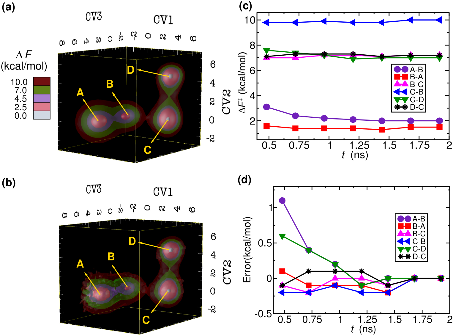
Refer to caption — Figure 1: (a) Three–dimensional model potential with four minima used to test the TASS method, visualized as contour surfaces; (b) Free energy surface reconstructed using the TASS method; (c) Free energy barriers computed from TASS as a function of simulation time per umbrella window; (d) Exact error in the free energy barrier estimates as a function of simulation time per umbrella window.

Temperature acceleration was then invoked along all the auxiliary variables $\{s_{\alpha}\}$ . The system temperature was set to 300 K, while that of the auxiliary variables was set to $600$ K. Temperature of the system and that of the auxiliary variables were maintained using two separate Langevin thermostats with frictional coefficients $0.02$ fs^-1 and $0.04$ fs^-1, respectively. Auxiliary variables $s_{1}$ and $s_{2}$ were (arbitrarily) chosen for applying US and MTD biases, respectively. Umbrella potentials were placed along $s_{1}$ from $-0.5$ Bohr to $6.5$ Bohr at intervals of $0.5$ Bohr. Initial structure for any given umbrella window was generated by setting the $s1$ coordinate to that corresponding to the equilibrium value of the umbrella window, while the other coordinates were having the same values as in the minimum A. Restraining potential $\kappa_{h}$ used for all the umbrella potentials was $31.4$ kcal mol^-1 Bohr^-2. The initial Gaussian height ( $w_{0}$ ) was set to $0.6$ kcal mol^-1 and the Gaussian width parameter $\delta s$ was $0.5$ Bohr. The parameter $\Delta T$ was taken as $1200$ K. MTD bias potential was updated every $200$ MD steps.

The convergence of free energy barriers as a function of simulation length (per umbrella window) is shown in Table SI2 and Figure 1c. From Figure 1d, it is clear that the free energy estimates converge to the exact result with increase in simulation time. The converged free energy surface is also plotted in Figure 1b. Positions of these minima and the topology of the potential energy surface are correctly reproduced in the reconstructed free energy surface.

These results show that a free energy surface with multiple minima and complex topology can be efficiently explored by the TASS method. Moreover, the free energy estimates systematically converge to the exact results.

III.2 Alanine Tripeptide

The free energy surface of alanine tripeptide (Figure 2a) in vacuo as a function of four backbone angles $(\phi 1,\psi 1,\phi 2,\psi 2)$ is explored here. Alanine tripeptide was modeled using the ff14SB force–field [40] and MD simulations were carried out using the PLUMED–AMBER interface. [41, 42] The time step was chosen as $1.0$ fs.

Here, umbrella bias was applied along the $\phi 1$ while MTD bias was applied along the $\phi 2$ . All the four coordinates were sampled using high temperature. MTD bias potentials were updated every $500$ fs and the parameters $w_{0}=0.6$ kcal mol^-1, $\delta s=0.05$ radians and $\Delta T=900$ K were taken. Umbrella potentials were placed from $-\pi$ to $\pi$ at an interval of $0.2$ radians with $\kappa_{\rm h}=1.2\times 10^{2}$ kcal mol^-1 rad^-2, $k_{\alpha}=1.2\times 10^{3}$ kcal mol^-1 rad^-2, and a mass of $50$ a.m.u. Å² rad^-2 was assigned to all the auxiliary variables.

Initial structure for any given umbrella window was generated arbitrarily by setting the $\phi 1$ internal coordinate to the equilibrium of the umbrella window, while the other collective variables were corresponding to the minimum P. Langevin thermostat with a frictional coefficient of $0.001$ fs^-1 was used for maintaining the temperature of physical system at $300$ K. An overdamped Langevin thermostat with a friction coefficient of $0.1$ fs^-1 was used to maintain the CV temperature at $900$ K. Before starting a TASS simulation, we carried out equilibration at $300$ K for a particular umbrella window for about $100$ ps.

For the purpose of comparison, we performed about $1$ $\mu s$ long replica exchange molecular dynamics (REMD) using AMBER 12. Four replicas at temperatures $300$ K, $365$ K, $440$ K, and $535$ K were chosen. Each replica was first equilibrated at its target temperature for $1$ ns. An exchange attempt between replica was made at every $10$ ps.

The free energy surface along the ( $\phi_{1}$ , $\phi_{2}$ ) coordinates computed from the REMD simulations is given in Figure 2d. Six major minima were obtained, labeled as P, Q, R, S, T, and U. Subsequently, we carried out TASS simulation with four collective variables as mentioned before ( $\phi 1$ , $\psi 1$ , $\phi 2$ , $\psi 2$ ). Computed free energy barriers separating these minima as a function of simulation time is plotted in Figure 2b. The barriers systematically converge, with an error less than 0.1 kcal mol^-1, after 10 ps long simulation per umbrella window. The converged high dimensional surface is then projected to the ( $\phi 1$ , $\phi 2$ ) space; Figure 2c. Clearly, the positions of the minima and the saddles are very well reproduced from TASS. Moreover, the diagonal symmetry of the landscape can also be noticed, showing that the exploration of the high dimensional free energy landscape has been performed very efficiently. Similar observations were also made when the free energy surface was projected along the ( $\phi 1$ , $\psi 1$ ) and ( $\phi 2$ , $\psi 2$ ); see Figure SI1. As free energy barriers could not be accurately computed from the REMD results (due to the insufficient sampling near the saddle points), we compare the free energy difference between the minima obtained from REMD and TASS; see Figure 2e and Table SI3. After convergence, the maximum difference between the REMD and the TASS results is only $~0.6$ kcal mol^-1, and this difference is likely due to the insufficient sampling in REMD. These results further support that TASS can efficiently explore the high dimensional free energy landscapes and provide converged free energy estimates in a computationally efficient way.

III.3 1,3–Butadiene to Cyclobutene Reaction

Here we explore the broad free energy surface for the conversion of 1,3–butadiene to cyclobutene which occurs via an electrocyclic reaction (see also Figure 3a).

We have chosen the following collective variables to model this reaction: a) distance C₁–C₄, $d[\mathrm{C}_{1}-\mathrm{C}_{4}]$ ; b) the distance C₁–C₂, $d[\mathrm{C}_{1}-\mathrm{C}_{2}]$ ; c) the distance C₂–C₃, $d[\mathrm{C}_{2}-\mathrm{C}_{3}]$ .

In TASS simulations, umbrella bias was applied along the $d$ [C₁–C₄] coordinate and MTD bias was applied along $d[\mathrm{C}_{1}-\mathrm{C}_{2}]$ . Auxiliary variables corresponding to all the three coordinates were sampled using high temperature. Simulations were carried out using ab initio MD employing plane–wave Kohn-Sham density functional theory (DFT) as available in the CPMD program. [43] PBE exchange correlation functional [44] with ultrasoft pseudopotential [45] was used here. A cutoff of 30 Ry was used for the plane–wave expansion of wavefunctions. System was taken in a cubic supercell of side length $15$ Å. Car–Parrinello [46] MD at $300$ K was carried out with a time step of $0.096$ fs and fictitious masses of orbitals were taken as $600$ a.u.

The parameter $k_{\alpha}$ was set to $1.2\times 10^{3}$ kcal mol^-1 Å^-2 and $\mu_{\alpha}$ was $50.0$ a.m.u. Langevin thermostat with a friction coefficient of $0.4$ fs^-1 was used to maintain the temperature of the extended degrees of freedom to $600$ K. In our simulations, $w_{0}=0.6$ kcal mol^-1 and $\delta s=0.05$ Bohr were taken. MTD bias was updated every $19$ fs. In US, the umbrella windows were placed from 1.5 Å to 3.9 Å at an interval of 0.05 Å with $\kappa_{\rm h}=4.4\times 10^{2}$ kcal mol^-1 Å^-2. Before starting the TASS simulation, each umbrella was equilibrated for about $2$ ps, and the initial structure for each umbrella window was obtained arbitrarily, as done in the case of alanine tripeptide.

We compare the results of the TASS simulation with the free energy surface and the barriers computed using the WS-MTD approach from our earlier work. [37] Free energy barriers converge to less than 0.5 kcal mol^-1 (in comparison with the WS-MTD barriers) within 10 ns per umbrella window; see Figure 3d,e. Simulation for 5 ps seems enough to compute the free energy barriers with an error less than 0.5 kcal mol^-1 (see Table SI4 ). The converged difference in the barriers of about 0.25 kcal mol^-1 could be ascribed to the differences in the type and the number of collective variables used in TASS and WS-MTD.

These results show that the TASS approach could efficiently sample a high dimensional free energy landscape in three collective variable space of a chemical reaction. The method seems to be as accurate as the WT-MTD, and is much efficient than the ordinary well-tempered MTD approach where free energy barriers for the same reaction was found not to converge even after $1000$ ps. [37]

III.4 Tetrahedral Intermediate Formation during Hydrolysis of Aztreonam and Class–C $\beta$ –Lactamase complex

To further demonstrate the application of the TASS method, we have applied this to model an enzymatic reaction in a DFT based QM/MM MD simulation. Here we model the formation of a tetrahedral intermediate during the hydrolysis of the covalent complex formed by aztreonam drug and Class–C $\beta$ –Lactamase; see Figure 4. Four collective variables were chosen for simulating this hydrolysis reaction (see Figure 4 for labeling): a) coordination number of ${\rm Tyr_{150}}$ O_η to hydrogens of W₁, $C[{{\rm Tyr}_{150}}{\rm O}_{\eta}-{\rm W_{1}H}]$ ; b) distance between ${\rm Azt}$ C2 and ${\rm W_{1}O}$ , $d[\rm{\rm AztC2}-{\rm W_{1}O}]$ ; c) the distance ${\rm Tyr_{150}}$ O_η to Lys₆₇N_ζ, $d[{\rm Tyr_{150}O}_{\eta}-{\rm Lys_{67}N}_{\zeta}]$ ; d) the distance ${\rm Tyr_{150}}$ O_η to Lys₃₁₅N_ζ, $d[{\rm Tyr_{150}O}_{\eta}-{\rm Lys_{315}N}_{\zeta}]$ . Here

C[{{\rm Tyr}_{150}}{\rm O}_{\eta}-{\rm W_{1}H}]=\sum_{J\in\rm W_{1}H}\frac{1}{\left(1+\left(\frac{d_{J}}{d_{0}}\right)^{6}\right)}

where $d_{J}\equiv d[{\rm Tyr}_{150}{\rm O}_{\eta}-{\mathrm{W_{1}H}}]$ and $d_{0}=1.3$ Å. The auxiliary variables corresponding to all the four collective variables were sampled using high temperature (1000 K), while the physical system was sampled at 300 K. Here $C[{{\rm Tyr}_{150}}{\rm O}_{\eta}-{\rm W_{1}H}]$ was chosen as a collective variable to accelerate proton transfer from water to Tyr₁₅₀O_η and MTD bias was applied along this collective variable. To enhance the nucleophilic attack of OH^- on the carbonyl carbon of the drug molecule $d[\rm{\rm AztC2}-{\rm W_{1}O}]$ coordinate was chosen as a collective variable which was sampled using the US bias. The collective variables $d[{\rm Tyr_{150}O}_{\eta}-{\rm Lys_{67}N}_{\zeta}]$ and $d[{\rm Tyr_{150}O}_{\eta}-{\rm Lys_{315}N}_{\zeta}]$ were considered for sampling different conformations of Tyr₁₅₀, Lys₆₇, and Lys₃₁₅.

The hybrid QM/MM simulations were performed using the CPMD/GROMOS interface [47] as implemented in the CPMD package. Aztreonam drug, side chains of Lys₆₇, Tyr₁₅₀, Ser₆₄, Lys₃₁₅, Thr₃₁₆; backbone of Lys₃₁₅, Thr₃₁₆, Gly₃₁₇, and two water molecules near the active site were treated quantum mechanically. Rest of the protein and the solvent molecules were treated by molecular mechanics (MM). The initial structure of the enzyme-drug complex was taken from the X–ray crystal structure corresponding to PDB ID 1FR6 [48]. This whole system is composed of the enzyme, $11391$ TIP3P water molecules, $2$ Na⁺ ions, and $2$ Cl^- ions, and was taken in a periodic simulation box with the size 81.3 $\times$ 75.6 $\times$ 64.5 Å³. Before starting the QM/MM simulation, MM MD simulation was carried out using the sander module in the AMBER suite of programs.[42] The whole protein was treated using parm99 AMBER force–field [49] whereas GAFF force–field [50] was employed for describing the drug molecule. Restrained electrostatic potential charges for drug and Ser₆₄ complex were computed using the RED software.[51] During classical simulation, a time step of $1$ fs and a cut–off distance of $15$ Å was used for non–bonded interaction. After initial steps of minimization, $1$ ns of $NPT$ simulation was carried out using Langevin thermostat at $300$ K and Berendsen barostat at $1$ atm. Subsequently, $10$ ns $NVT$ simulation was performed with the equilibrated density. In hybrid QM/MM simulations, QM part was treated using the plane–wave DFT with PBE exchange correlation functional. [44] Ultrasoft psuedopotentials [45] were chosen and a plane–wave cutoff of 25 Ry was used. A cubic QM box with a side length of 25.3 Å was taken. MM part of the system was treated using the param99 [49] AMBER force–field. Capping hydrogen atoms were added to saturate the bonds at the QM/MM boundary. Capping hydrogen atoms were introduced between C_β and C_γ atoms of Tyr₁₅₀, C_α and C_β atoms of Ser₆₄, C_γ and C_δ atoms of Lys₆₇, and C_α and N atoms of Lys₃₁₅ and Gly₃₁₇.

Constant temperature Car–Parrinello [46] MD at $300$ K was carried out using the Nos $\mathrm{\grave{e}}$ –Hoover chain thermostats for the nuclei and orbital degrees of freedom. [52] A time step of $0.14$ fs was used to integrate the equations of motion and the fictitious masses of orbitals were taken as 600 a.u. We assigned $k_{\alpha}=1.2\times 10^{3}$ kcal mol^-1 and $\mu_{\alpha}=50.0$ a.m.u. for all the auxiliary variables. An overdamped Langevin thermostat with a friction coefficient of $0.4$ fs^-1 was used to maintain temperature of the auxiliary variables at $1000$ K. In US, windows were placed from 1.3 Å to 5.1 Å at an interval of 0.1 Å with $\kappa_{\rm h}=4.5\times 10^{2}$ kcal mol^-1 Å^-2. The MTD parameters were $w_{0}=0.6$ kcal mol^-1, $\delta s=0.05$ Bohr and $\Delta T=2000$ K were taken. MTD bias was updated every $19$ fs.

Before starting the TASS simulations, each umbrella window was equilibrated for about $4$ ps. Initial structure for an umbrella window was taken from the adjacent equilibrated window. The whole protein, including the QM part, and the solvent molecules were free to move during the MD simulations.

We could successfully simulate the reaction EI1 $\rightarrow$ EP1 using the TASS method, and the converged reconstructed free energy surface is given in Figure 4b,c. Unlike in the previous benchmark cases, we have used varying simulation lengths (4-8 ps each) for different umbrella windows till a convergence in the free energy barrier was achieved. In the reactant basin, we have noticed proton transfer between Tyr₁₅₀ and Lys₆₇, i.e. EI1 $\leftrightarrow$ EI2. The hydrogen bonding interactions between the two residues were maintained throughout the reaction. However, distance between the Tyr₁₅₀O_η and Lys₆₇N_ζ increases as proton transfer occurs from W₁ to Tyr₁₅₀O_η; see Figure 4c. On the other hand, the hydrogen bonding interaction between Lys₃₁₅ and Tyr₁₅₀ was broken in the initial stages of the chemical reaction, as a result of which, another water molecule (W2) moved into the active site, and Lys₃₁₅ formed interactions with Glu₂₇₂.

The free energy barrier for the reaction was computed from the projected free energy surface on $d[{\rm Tyr_{150}O}_{\eta}-{\rm Lys_{67}N}_{\zeta}]$ and $C[{{\rm Tyr}_{150}}{\rm O}_{\eta}-{\rm W_{1}H}]$ coordinates, and is 24.5 kcal mol^-1. From experimental studies [53] it is known that aztreonam is a slowly hydrolyzing drug and from the measured rate constants for deacylation, we estimate the corresponding free energy barrier as 23 kcal mol^-1 (using the transition state theory). This agrees well with our computed free energy barrier of 24.5 kcal mol^-1.

The same reaction was failed to simulate in an ordinary MTD run, likely due to the broad nature of the basin along the $d[{\rm Tyr_{150}O}_{\eta}-{\rm Lys_{67}N}_{\zeta}]$ coordinate (see also Figure 4)c, and thus large computational time would be required to build the sufficient bias potential in the relevant parts of the free energy surface. Moreover, W₁ water molecule was also driven out of the active site, which was then replaced by an MM water molecule from the bulk (data not shown). Both these difficulties are overcome in the TASS simulation since US was carried out along the $d[{\rm Tyr_{150}O}_{\eta}-{\rm Lys_{67}N}_{\zeta}]$ coordinate. Additionally, sampling of different conformations of the active site residues needed four collective variables which is also practically difficult to sample properly with conventional MTD, especially in DFT based QM/MM simulations.

IV Conclusions

In this paper, we presented a method called TASS that combines MTD, US, and TAMD to sample large number of collective variables and explore high dimensional free energy landscapes. Free energy estimates using TASS is shown to converge systematically to the exact values. We have demonstrated the efficiency of TASS in sampling four and five dimensional free energy landscapes with multiple minima along different coordinates. Moreover, the method is also shown to be practically usable for computing free energy surfaces of chemical reactions in ab initio and DFT based hybrid QM/MM MD simulations.

The method is well suited for exploring free energy surfaces that are broad and unbound, where conventional enhanced sampling approaches such as MTD and TAMD become inefficient. Controlled exploration of free energy surfaces, for e.g. along certain reaction pathways, can also be achieved in TASS, by an appropriate choice of the US coordinate. The method permits one to add and remove collective variables in different umbrella windows, giving flexibility and computational efficiency in exploring complex high dimensional free energy landscapes. Although, we have used US and MTD biases, the method can be straightforwardly extended to the cases where MTD bias is not required (either in selected or for all the umbrella windows), by setting $A(\tau)=1$ in Equation (5). Replica exchange based algorithms can also be combined with TASS to further improve the sampling efficiency. The TASS Hamiltonian in Equation (4) can be realized effortlessly in simulations using MD plugins like PLUMED [41] which has been interfaced with several popular MM and QM programs.

Acknowledgements.

Authors thank IIT Kanpur for availing the HPC facility. SA thanks UGC for Ph. D fellowship.

References

[1] M. E. Tuckerman, Statistical Mechanics: Theory and Molecular Simulation, 1st ed. (Oxford University Press, Oxford, 2010).
[2] T. Leli $\grave{e}$ vre, M. Rousset, and G. Stoltz, Free Energy Computations: A Mathematical Perspective (Imperial College Press, London, 2010).
[3] E. Vanden-Eijnden, J. Comput. Chem. 30, 1737 (2009).
[4] C. D. Christ, A. E. Mark, and W. F. van Gunsteren, J. Comput. Chem. 31, 1569 (2010).
[5] C. Abrams and G. Bussi, Entropy 16, 163 (2014).
[6] R. D. Miller, Annu. Rev. Phys. Chem. 65, 583 (2014).
[7] O. Valsson, P. Tiwary, and M. Parrinello, Annu. Rev. Phys. Chem. 67, 159 (2016).
[8] A. Laio and M. Parrinello, Proc. Natl. Acad. Sci. 99, 12562 (2002).
[9] M. Iannuzzi, A. Laio, and M. Parrinello, Phys. Rev. Lett. 90, 238302 (2003).
[10] A. Barducci, M. Bonomi, and M. Parrinello, WIREs Comput. Mol. Sci. 1, 826 (2011).
[11] L. Sutto, S. Marsili, and F. L. Gervasio, WIREs: Comput. Mol. Sci. 2, 771 (2012).
[12] A. Laio and F. L. Gervasio, Rep. Prog. Phys. 71, 126601 (2008).
[13] G. M. Torrie and J. P. Valleau, Chem. Phys. Lett. 28, 578 (1974).
[14] J. Kästner, WIREs Comput. Mol. Sci. 1, 932 (2011).
[15] T. Huber, A. E. Torda, and W. F. van Gunsteren, J. Comput. Aided Mol. Des. 8, 695 (1994).
[16] H. Grubmüller, Phys. Rev. E 52, 2893 (1995).
[17] F. Wang and D. P. Landau, Phys. Rev. Lett. 86, 2050 (2001).
[18] E. Darve and A. Pohorille, J. Chem. Phys. 115, 9169 (2001).
[19] U. H. E. Hansmann and L. T. Wille, Phys. Rev. Lett. 88, 068105 (2002).
[20] M. Yang, L. Yang, Y. Gao, and H. Hu, J. Chem. Phys. 141, 044108 (2014).
[21] J. Comer, J. C. Gumbart, J. Hénin, T. Lelièvre, A. Pohorille, and C. Chipot, J. Phys. Chem. B 119, 1129 (2015).
[22] Y. I. Yang, J. Zhang, X. Che, L. Yang, and Y. Q. Gao, J. Chem. Phys. 144, 094105 (2016).
[23] A. Barducci, G. Bussi, and M. Parrinello, Phys. Rev. Lett. 100, 020603 (2008).
[24] J. F. Dama, M. Parrinello, and G. A. Voth, Phys. Rev. Lett. 112, 240602 (2014).
[25] G. Bussi, F. L. Gervasio, A. Laio, and M. Parrinello, J. Am. Chem. Soc. 128, 13435 (2006).
[26] S. Piana and A. Laio, J. Phys. Chem. B 111, 4553 (2007).
[27] F. Marinelli, F. Pietrucci, A. Laio, and S. Piana, PLOS Comput. Biol. 5, e1000452 (2009).
[28] A. Gil-Ley and G. Bussi, J. Chem. Theory Comput. 11, 1077 (2015).
[29] J. Pfaendtner and M. Bonomi, J. Chem. Theory Comput. 11, 5062 (2015).
[30] P. Shaffer, O. Valsson, and M. Parrinello, Proc. Natl. Acad. Sci. 113, 1150 (2016).
[31] A. M. Ferrenberg and R. H. Swendsen, Phys. Rev. Lett. 63, 1195 (1989).
[32] S. Kumar, D. Bouzida, R. H. Swendsen, P. A. Kollman, and J. M. Rosenberg, J. Comput. Chem. 13, 1011 (1992).
[33] L. Maragliano and E. Vanden-Eijnden, Chem. Phys. Lett. 426, 168 (2006).
[34] J. B. Abrams and M. E. Tuckerman, J. Phys. Chem. B 112, 15742 (2008).
[35] M. Chen, M. A. Cuendet, and M. E. Tuckerman, J. Chem. Phys. 137, 024102 (2012).
[36] M. Chen, T.-Q. Yu, and M. E. Tuckerman, Proc. Natl. Acad. Sci. 112, 3235 (2015).
[37] S. Awasthi, V. Kapil, and N. N. Nair, J. Comput. Chem. 37, 1413 (2016).
[38] M. Bonomi, A. Barducci, and M. Parrinello, J. Comput. Chem. 30, 1615 (2009).
[39] P. Tiwary and M. Parrinello, J. Phys. Chem. B 119, 736 (2014).
[40] J. A. Maier, C. Martinez, K. Kasavajhala, L. Wickstrom, K. E. Hauser, and C. Simmerling, J. Chem. Theory Comput. 11, 3696 (2015).
[41] M. Bonomi, D. Branduardi, G. Bussi, C. Camilloni, D. Provasi, P. Raiteri, D. Donadio, F. Marinelli, F. Pietrucci, R. A. Broaglia, and M. Parrinello, Comput. Phys. Commun. 180, 1961 (2009).
[42] D. A. Case, T. A. Darden, T. E. Cheatham, C. L. Simmerling, J. Wang, R. E. Duke, R. Luo, R. C. Walker, W. Zhang, K. M. Merz, B. Roberts, S. Hayik, A. Roitberg, G. Seabra, J. Swails, A. W. Goetz, I. Kolossváry, K. F. Wong, F. Paesani, J. Vanicek, R. M. Wolf, J. Liu, X. Wu, S. R. Brozell, T. Steinbrecher, H. Gohlke, Q. Cai, X. Ye, J. Wang, M. J. Hsieh, G. Cui, D. R. Roe, D. H. Mathews, M. G. Seetin, R. Salomon-Ferrer, C. Sagui, V. Babin, T. Luchko, S. Gusarov, A. Kovalenko, and P. A. Kollman, AMBER 12 (University of California, San Francisco, 2012).
[43] Version 13.2, CPMD Program Package, IBM Corp 1990-2011, MPI für Festkörperforschung Stuttgart 1997-2001.
[44] J. P. Perdew, J. A. Chevary, S. H. Vosko, K. A. Jackson, M. R. Pederson, D. J. Singh, and C. Fiolhais, Phys. Rev. B 46, 6671 (1992).
[45] D. Vanderbilt, Phys. Rev. B 41, 7892 (1990).
[46] R. Car and M. Parrinello, Phys. Rev. Lett. 55, 2471 (1985).
[47] A. Laio, J. VandeVondele, and U. Rothlisberger, J. Chem. Phys. 116, 6941 (2002).
[48] C. Oefner, A. D’Arcy, J. J. Daly, K. Gubernator, R. L. Charnas, I. Heinze, C. Hubschwerlen, and F. K. Winkler, Nature 343, 284 (1990).
[49] T. E. Cheatham III, P. Cieplak, and P. A. Kollman, J. Biomol. Struct. Dyn. 16, 845 (1999).
[50] J. Wang, R. M. Wolf, J. W. Caldwell, P. A. Kollman, and D. A. Case, J. Comput. Chem. 25, 1157 (2004).
[51] RED: RESP ESP Charge Derive, version III.3; see http://q4md-forcefieldtools.org/RED/.
[52] G. J. Martyna, M. L. Klein, and M. Tuckermann, J. Chem. Phys. 97, 2635 (1992).
[53] D. Monnaie, R. Virden, and J. M. Fr $\grave{e}$ re, FEBS Letters 306, 108 (1992).