Modeling Tangential Vector Fields on a Sphere

Minjie Fan ^†^†thanks: Corresponding author. Affiliation: Department of Statistics, University of California, Davis Debashis Paul Affiliation: Department of Statistics, University of California, Davis Thomas C.M. Lee Affiliation: Department of Statistics, University of California, Davis Tomoko Matsuo Affiliation: Cooperative Institute for Research in Environmental Sciences, University of Colorado, Boulder

Abstract

Physical processes that manifest as tangential vector fields on a sphere are common in geophysical and environmental sciences. These naturally occurring vector fields are often subject to physical constraints, such as being curl-free or divergence-free. We construct a new class of parametric models for cross-covariance functions of curl-free and divergence-free vector fields that are tangential to the unit sphere. These models are constructed by applying the surface gradient or the surface curl operator to scalar random potential fields defined on the unit sphere. We propose a likelihood-based estimation procedure for the model parameters and show that fast computation is possible even for large data sets when the observations are on a regular latitude-longitude grid. Characteristics and utility of the proposed methodology are illustrated through simulation studies and by applying it to an ocean surface wind velocity data set collected through satellite-based scatterometry remote sensing. We also compare the performance of the proposed model with a class of bivariate Matérn models in terms of estimation and prediction, and demonstrate that the proposed model is superior in capturing certain physical characteristics of the wind fields.

Keywords: curl-free, divergence-free, Helmholtz-Hodge decomposition, Matérn model, ocean surface wind

1 Introduction

Vector fields defined on a spherical domain are principal objects of study in many branches of science. Terrestrial physical processes such as wind and oceanic currents, gravity, electric and magnetic fields are some of the most well-studied examples. In meteorology, the directionality of wind flow at surface level is an example of a tangential vector field defined on a sphere (Earth’s surface). Because the effective portion of the atmosphere and the oceans are considerably thinner in their vertical extent in comparison with their horizontal extent, for many geophysical processes, the horizontal scale far exceeds the vertical scale. It is therefore natural to decompose such vector fields into tangential and radial components and treat them separately. For example, velocity divergence is expressed as the sum of horizontal (tangential) and vertical (radial) divergence in the continuity equation. Other such examples of vector fields include electric and magnetic fields in geophysics (Sabaka et al.,, 2010). A branch of solid-Earth geophysics focuses on the behavior of the Earth’s magnetic field, while its interactions with the solar wind are the focus of science of space weather. Electric and magnetic fields associated with ionospheric electric currents are distinct in the tangential direction from the radial direction, and many of the ionospheric electrodynamic processes can be treated as tangential vector fields on a sphere (Richmond and Kamide,, 1988). In this paper, we focus on modeling the tangential component of vector fields on the unit sphere, especially its small-scale stochastic variations, which can form a significant part of the overall variability. Accounting for this variability can enhance prediction accuracy of models, enable subgrid-scale inference, and facilitate better uncertainty quantification of model parameters. The modeling framework that we propose is flexible, incorporates small-scale variations, and is naturally interpretable and computationally tractable.

Gaussian random fields (GRF) have provided a very successful modeling framework for describing variations in many physical processes. Two key ingredients of the success of GRF modeling for stochastic processes are: (i) the behavior of the process is entirely characterized by the mean and the covariance functions, thereby facilitating deep theoretical investigations; and (ii) computations for both estimation and prediction primarily involve matrix algebra. We provide a very brief overview of existing literature on the construction of covariance functions and random fields on a sphere. Marinucci and Peccati, (2011) gave a detailed account of weakly isotropic processes on the unit sphere, while Guinness and Fuentes, (2015) gave a broad overview of spherical processes. Hitczenko and Stein, (2012) Jun, (2011), Jun and Stein, (2007), Jun and Stein, (2008) mostly focused on the construction and characterization of covariance functions of Gaussian processes on the unit sphere.

Extension of the modeling framework from scalar random fields to random vector fields poses an additional challenge due to the requirement of non-negative definiteness for the cross-covariance function of the vector fields. Popular approaches to modeling vector fields include linear coregionalization models (Bourgault and Marcotte,, 1991; Gelfand et al.,, 2004; Goulard and Voltz,, 1992), the multivariate Matérn model (Apanasovich et al.,, 2012; Gneiting et al.,, 2010), and models derived from scalar potentials through differential operators (Jun,, 2011; Jun,, 2014); the latter being especially notable for their constructive approach. However, these models do not impose specific physical constraints on the Cartesian components of the vector fields. There are many examples of vector fields satisfying “natural” physical constraints. For example, magnetic fields are solenoidal with zero divergence, and electric fields resulting from electric charges are curl-free. Vorticity, defined as the curl of a velocity vector field, plays an important role in atmospheric and oceanic dynamics in terms of characterizing the nature and degree of turbulence. Assuming water is incompressible, Zhang et al., (2007) represented lake water current velocity fields through applying the curl operator to a scalar stream function. Constantinescu and Anitescu, (2013) developed cross-covariance models that incorporate known physical constraints relating the behavior of their Cartesian components, and demonstrated that physics-based models can significantly outperform independence models in an application to geostrophic winds. These examples indicate that kriging or data assimilation for observations of geophysical and environmental processes will benefit from modeling vector fields as Gaussian processes that incorporate constraints such as curl-free or divergence-free into their construction.

We illustrate the basic characteristics of a vector field with physical constraints through Figure 1, which shows an example of a pair of simulated divergence-free and curl-free random fields using models that will be presented later in this paper. The details of how these fields are simulated will be described in Section 3.1.

Refer to caption — Figure 1: Simulated divergence-free and curl-free random fields on the HEALPix grid. The sphere has been projected to an ellipse by the Hammer projection. Using the same set of random deviates, these fields are simulated based on the Cholesky decomposition. The details will be described in Section 3.1.

Modeling and analysis of vector fields (not necessarily tangential to a sphere) is facilitated by the celebrated Helmholtz-Hodge decomposition (Freeden and Schreiner,, 2009; Kadri-Harouna and Perrier,, 2012) that expresses the vector field as the sum of a curl-free component, a divergence-free component and a component that is the gradient of a harmonic function. The harmonic component vanishes when the domain is a spherical surface and the vector field is tangential to this surface. In Section 2, we define the basic objects such as surface gradient and surface curl operators that are fundamental to the construction of a curl-free or a divergence-free component. Our work is related to that of Scheuerer and Schlather, (2012), who constructed random vector fields that are either curl-free or divergence-free, and that of Schlather et al., (2015) who introduced a parametric cross-covariance model for random vector fields consisting of the aforementioned curl-free and divergence-free components. However, these constructions are restricted to vector fields defined on Euclidean spaces only.

In this paper, we construct Gaussian tangential vector fields on the unit sphere that are either curl-free or divergence-free. We then utilize the Helmholtz-Hodge decomposition to construct general Gaussian tangential vector fields from a pair of correlated Gaussian scalar potential fields. These constructions involve making careful use of the spherical geometry and appropriate differential operators on the unit sphere. Through specifying a bivariate Matérn model for the pair of potential fields, we propose a simple but flexible parametric model named Tangent Matérn Model (TMM) with the following characteristics:

(i)

There is a parameter controlling the correlation between the curl-free and the divergence-free components of the model, which is often non-zero for wind velocity fields (Cornford,, 1998).
(ii)

The vector field can be equivalently represented in terms of its zonal and meridional components, and in this form, it allows for a negative correlation between two locations, which is common in meteorological variables (Daley,, 1991, Chapter 4.3).
(iii)

The vector field is modeled as the sum of a curl-free and a divergence-free components. The magnitude of each component, which is related to two important physical characteristics of the vector field, divergence and vorticity, can be inferred from the parameter estimates.
(iv)

The cross-covariance structure of the vector field is not isotropic but axially symmetric.

We then propose a likelihood-based estimation procedure for the TMM and study its characteristics in terms of estimation through a simulation study. We also present a fast computational algorithm that is applicable when the data are observed on a regular latitude-longitude grid. The proposed modeling framework, which is primarily used to describe the small-scale features of a vector field, is also extended to describe large-scale and spatio-temporal variability.

As an illustration, we apply the proposed methodology to a data set on ocean surface wind velocities obtained from a satellite survey conducted by NASA’s Quick Scatterometer (QuikSCAT) satellite. Scatterometer data are important for numerical weather prediction. Through the data assimilation process of surface winds, the analysis of the atmospheric mass and motion fields above the surface can be improved, which increases the accuracy of weather forecasts. Scatterometer data also contribute to improved storm warning and monitoring (Atlas et al.,, 2001; Brennan et al.,, 2009). Over the past two decades, a number of statistical methods have been applied to modeling wind fields. For example, Wikle and Cressie, (1999) demonstrated that enhancement in prediction accuracy of spatio-temporal Kalman filtering is possible through careful incorporation of small-scale stochastic variations into the model. Wikle et al., (2001) proposed a spatio-temporal hierarchical Bayesian model for tropical ocean surface winds, where the model includes small-scale wind components that are represented in terms of wavelet basis functions. Reich and Fuentes, (2007) developed a multivariate semiparametric Bayesian spatial model for hurricane surface wind fields based on the stick-breaking prior, while Foley and Fuentes, (2008) applied a linear coregionalization model to the zonal and meridional components of hurricane surface wind fields. Also, Cornford et al., (2004) fitted a version of the model of Schlather et al., (2015) using a Matérn covariance function to surface wind fields over a small sector of the north Atlantic ocean, by making planar approximation to the spherical surface. Due to the many-faceted complexity of the data, intricacies of the available scientific models, and space limitation, full-scale modeling of surface wind velocity fields is beyond the scope of this paper. Instead, we focus here primarily on the characteristics of the residual fields after removing large-scale components through an empirical orthogonal function (EOF) analysis, and demonstrate the implications of using the TMM for fitting such fields. We also compare the predictive performance of co-kriging based on the proposed TMM and a parsimonious bivariate Matérn model (Gneiting et al.,, 2010). The results show that the TMM performs better in terms of both estimation and prediction, which can be attributed to its ability of capturing the physical characteristics of the wind fields.

The remainder of the paper is organized as follows. In Section 2, we present the constructions of curl-free and divergence-free random tangential vector fields and the TMM. The details of model fitting are also discussed in this section. We conduct numerical experiments in Section 3 to show the good performance of parameter estimation and spatial prediction. The TMM is applied to a QuikSCAT ocean surface wind velocity data set in Section 4. We discuss some relevant issues and future directions in Section 5.

2 Construction of Random Tangential Vector Fields

2.1 Surface Gradient and Surface Curl Operators

Tangential vector fields on the unit sphere can be constructed by applying appropriate differential operators to scalar potential fields. Let $\mathbf{s}$ denote a point on the unit sphere $\mathbb{S}^{2}=\{\mathbf{x}\in\mathbb{R}^{3}:\lVert\mathbf{x}\rVert=1\}$ and $(\theta,\phi)$ represent the same in the spherical coordinate system, where $\theta$ and $\phi$ are the co-latitude and longitude, respectively. The tangent space at $\mathbf{s}\equiv(\theta,\phi)$ , to be denoted by ${\cal T}_{\mathbf{s}}$ , is a two-dimensional vector space with canonical orthonormal basis vectors $\hat{\bm{\theta}}$ and $\hat{\bm{\phi}}$ . These two vectors are defined such that $\hat{\bm{\theta}}$ is tangent to the great circle passing through the poles and $\mathbf{s}$ , and it points to the south pole, while $\hat{\bm{\phi}}$ points eastward along the circle that is the intersection of $\mathbb{S}^{2}$ with a plane passing through $\mathbf{s}$ and parallel to the equatorial plane. Moreover, let $\hat{\mathbf{r}}$ be a unit vector at $\mathbf{s}$ that points radially outward, i.e., $\hat{\mathbf{r}}=\hat{\bm{\theta}}\times\hat{\bm{\phi}}$ , where $\times$ denotes the cross product on $\mathbb{R}^{3}$ . All the vectors vary with $\mathbf{s}$ , but for the moment we suppress this. In order to define spherical differential operators based on usual differential operators on $\mathbb{R}^{3}$ , for any function or random field on $\mathbb{S}^{2}$ mentioned hereafter, we always assume that it is actually defined on some spherical shell containing $\mathbb{S}^{2}$ , $S_{\epsilon}=\{\mathbf{x}\in\mathbb{R}^{3}:1-\epsilon<\lVert\mathbf{x}\rVert<1+\epsilon\}$ , where $\epsilon>0$ .

For the unit sphere, the surface gradient of a continuously differentiable function $f:\mathbb{S}^{2}\to\mathbb{R}$ is defined as the tangential component of its usual gradient

\nabla_{\mathbf{s}}^{*}f=:\mathbf{P}_{\mathbf{s}}\nabla_{\mathbf{s}}f,

where $\mathbf{s}=(s_{1},s_{2},s_{3})^{\rm T}\in\mathbb{S}^{2},\mathbf{P}_{\mathbf{s}}=\mathbf{I}_{3}-\mathbf{s}\mathbf{s}^{\rm T}$ is the matrix that projects a vector in $\mathbb{R}^{3}$ onto $\mathcal{T}_{\mathbf{s}}$ , and $\nabla_{\mathbf{s}}$ is the usual gradient. Then the surface curl of $f$ is defined as a tangential vector field perpendicular to $\nabla_{\mathbf{s}}^{*}f$

L_{\mathbf{s}}^{*}f=:\hat{\mathbf{r}}\times\nabla_{\mathbf{s}}^{*}f=\mathbf{Q}_{\mathbf{s}}\nabla_{\mathbf{s}}f,

where the matrix $\mathbf{Q}_{\mathbf{s}}$ is defined in (18) of Appendix A.

If we further assume that $f$ is twice continuously differentiable, then $\nabla^{*}_{\mathbf{s}}f$ and $L_{\mathbf{s}}^{*}f$ are curl-free and divergence-free, respectively, i.e., $\mathrm{curl}_{\mathbf{s}}^{*}(\nabla^{*}_{\mathbf{s}}f)=:L_{\mathbf{s}}^{*}\cdot\nabla^{*}_{\mathbf{s}}f=0$ , where $\cdot$ denotes the dot (or scalar) product, and $\mathrm{div}_{\mathbf{s}}^{*}(L_{\mathbf{s}}^{*}f)=:\nabla_{\mathbf{s}}^{*}\cdot L_{\mathbf{s}}^{*}f=0$ . If $f$ is only continuously differentiable, $\mathrm{curl}_{\mathbf{s}}^{*}(\nabla^{*}_{\mathbf{s}}f)$ and $\mathrm{div}_{\mathbf{s}}^{*}(L_{\mathbf{s}}^{*}f)$ are not well-defined in the ordinary sense, and hence we call $\nabla^{*}_{\mathbf{s}}f$ the gradient-field and $L_{\mathbf{s}}^{*}f$ the curl-field derived from $f$ . More details on differential calculus on the unit sphere can be found in Chapter 2 of Freeden and Schreiner, (2009). Some auxiliary notations and definitions are given in Appendix A.

2.2 Construction of Curl-free and Divergence-free Random Tangential Vector Fields

In this subsection, we present an approach for constructing curl-free and divergence-free random tangential vector fields on the unit sphere. These vector fields are derived by applying the surface gradient and the surface curl operators to a scalar random potential field, to be generically denoted by $Z(\mathbf{s})$ . The cross-covariance structure of the derived vector fields will be determined by the covariance structure of the process $Z$ . Suppose $Z$ is defined on $S_{\epsilon}$ with mean zero and finite variance, and satisfies the following regularity conditions:

A1

The process $Z(\mathbf{s})$ is differentiable in quadratic mean. Moreover, there exists a $\mathbb{P}-$ a.e. sample continuously differentiable version of $Z$ , denoted by $\widetilde{Z}$ , such that $D^{(i)}\widetilde{Z}(\mathbf{s})=D_{\mathrm{qm}}^{(i)}Z(\mathbf{s})$ $\mathbb{P-}$ a.e., where $D^{(i)}$ and $D^{(i)}_{\rm qm}$ represent the sample partial derivative and the partial derivative in quadratic mean along the $i$ -th coordinate direction, respectively.
A2

The process $Z(\mathbf{s})$ is stationary with twice continuously differentiable covariance function $C(\mathbf{h})$ , where $\mathbf{h}$ is the spatial separation vector between $\mathbf{s}$ and $\mathbf{t}$ , i.e., $\mathbf{h}=\mathbf{s}-\mathbf{t}$ .

The two regularity conditions ensure the validity of applying the differential operators. When $Z(\mathbf{s})$ is Gaussian, A1 can be verified through Theorems 3.2 and 4.3 in Potthoff, (2010). By A1, there exists $\Omega_{0}\subset\Omega$ with $\mathbb{P}(\Omega_{0})=1$ such that $\widetilde{Z}(\mathbf{s},\omega)$ is continuously differentiable on $S_{\epsilon}$ for any $\omega\in\Omega_{0}$ . By applying the differential operators to $\widetilde{Z}$ , which can be seen as a scalar random potential field, we construct two random tangential vector fields $\mathbf{Y}_{\mathrm{curl},Z}$ and $\mathbf{Y}_{\mathrm{div},Z}$ on $\mathbb{S}^{2}$ such that $\mathbf{Y}_{\mathrm{curl},Z}(\mathbf{s},\omega)=\mathbf{P}_{\mathbf{s}}\nabla_{\mathbf{s}}\widetilde{Z}(\mathbf{s},\omega)$ and $\mathbf{Y}_{\mathrm{div},Z}(\mathbf{s},\omega)=\mathbf{Q}_{\mathbf{s}}\nabla_{\mathbf{s}}\widetilde{Z}(\mathbf{s},\omega)$ for any $\omega\in\Omega_{0}$ . It is clear that the sample paths of $\mathbf{Y}_{\mathrm{curl},Z}$ and $\mathbf{Y}_{\mathrm{div},Z}$ are gradient-fields and curl-fields $\mathbb{P}-$ a.e., respectively. If we further assume that the sample paths of $\widetilde{Z}$ are twice continuously differentiable $\mathbb{P}-$ a.e., then $\mbox{curl}_{\mathbf{s}}^{*}(\mathbf{Y}_{\mathrm{curl},Z}(\mathbf{s},\omega))$ and $\mbox{div}_{\mathbf{s}}^{*}(\mathbf{Y}_{\mathrm{div},Z}(\mathbf{s},\omega))$ are well-defined and equal to zero for any $\omega\in\Omega_{0}$ , and hence $\mathbf{Y}_{\mathrm{curl},Z}$ and $\mathbf{Y}_{\mathrm{div},Z}$ are curl-free and divergence-free, respectively.

The cross-covariance functions of $\mathbf{Y}_{\mathrm{curl},Z}$ and $\mathbf{Y}_{\mathrm{div},Z}$ , to be denoted by $\mathbf{C}_{\mathrm{curl},Z}$ and $\mathbf{C}_{\mathrm{div},Z}$ , respectively, are given explicitly in Theorem 1, the proof of which appears in Appendix B.

Theorem 1.

If A1 and A2 hold, then the cross-covariance functions $\mathbf{C}_{\mathrm{curl},Z}$ and $\mathbf{C}_{\mathrm{div},Z}$ can be represented as

\mathbf{C}_{\mathrm{curl},Z}(\mathbf{s},\mathbf{t})=-\mathbf{P}_{\mathbf{s}}\nabla_{\mathbf{h}}\nabla_{\mathbf{h}}^{\rm T}C(\mathbf{h})\bigg|_{\mathbf{h}=\mathbf{s}-\mathbf{t}}\mathbf{P}_{\mathbf{t}}^{\rm T},

(1)

and

\mathbf{C}_{\mathrm{div},Z}(\mathbf{s},\mathbf{t})=-\mathbf{Q}_{\mathbf{s}}\nabla_{\mathbf{h}}\nabla_{\mathbf{h}}^{\rm T}C(\mathbf{h})\bigg|_{\mathbf{h}=\mathbf{s}-\mathbf{t}}\mathbf{Q}_{\mathbf{t}}^{\rm T}.

(2)

We consider a special case of the construction described above, where $Z(\mathbf{s})$ is an isotropic scalar random field on $S_{\epsilon}$ , so that its covariance function $C(\mathbf{h})$ can be written as $C_{1}(\lVert\mathbf{h}\rVert)$ , where $C_{1}(r)$ is a function from $[0,2+2\epsilon)$ to $\mathbb{R}$ . One popular choice for $C_{1}$ is the Matérn model

M(r;\nu,a)=\frac{2^{1-\nu}}{\Gamma(\nu)}(ar)^{\nu}K_{\nu}(ar),

(3)

where $K_{\nu}$ is the modified Bessel function of the second kind, the parameter $\nu>0$ controls the smoothness, and $a>0$ is the spatial scale parameter, whereby $1/a$ controls the range of correlation. When $Z(\mathbf{s})$ is assumed to be Gaussian with covariance function $C_{1}(\lVert\mathbf{h}\rVert)=M(\lVert\mathbf{h}\rVert;\nu,a)$ , $\nu>1$ is necessary and sufficient to ensure that conditions A1 and A2 hold. We give a proof of the statement in Appendix C, and explicit expressions of $\nabla_{\mathbf{h}}\nabla_{\mathbf{h}}^{\rm T}C_{1}(\lVert\mathbf{h}\rVert)$ in Appendix D.

We now establish connections of our proposal with existing literature. Narcowich et al., (2007) and Fuselier and Wright, (2009) constructed a general class of positive definite curl-free and divergence-free kernels on $\mathbb{S}^{2}$ using radial basis functions (RBFs) on $\mathbb{R}^{3}$ . The cross-covariance kernels defined in (1) and (2), when $Z(\mathbf{s})$ is isotropic, belong to this class. However, the constructions of Narcowich et al., (2007) and Fuselier and Wright, (2009) are deterministic in nature, and the descriptions of their kernels do not automatically lead to the construction of random tangential vector fields. In contrast, our construction takes a different path, by directly deriving vector fields through the application of differential operators to scalar random potential fields. Moreover, we can extend the basic framework presented here to construct a rich class of spatio-temporal tangential vector fields on the unit sphere with more complicated cross-covariance structures and including large-scale components. These ideas will be developed in two stages, first by constructing a tangential vector field with correlated curl-free and divergence-free components from a pair of correlated scalar random potential fields (Section 2.3), and then by extending the framework to spatio-temporal processes (Section 2.5).

2.3 Tangent Matérn Model

In this subsection, we construct a class of Gaussian tangential vector fields by making use of the Helmholtz-Hodge decomposition and the ingredients developed in Section 2.2. Let $\mathbf{Z}(\mathbf{s})=(Z_{1}(\mathbf{s}),Z_{2}(\mathbf{s}))^{\rm T}$ denote an isotropic, bivariate, Gaussian random field on $S_{\epsilon}$ with mean zero and cross-covariance function $\mathbf{C}(\lVert\mathbf{h}\rVert)=\mbox{Cov}(\mathbf{Z}(\mathbf{s}),\mathbf{Z}(\mathbf{t}))$ , where $\mathbf{h}=\mathbf{s}-\mathbf{t}$ and $\mathbf{s},\mathbf{t}\in S_{\epsilon}$ . The Helmholtz-Hodge decomposition states that any continuously differentiable tangential vector field on $\mathbb{S}^{2}$ can be uniquely decomposed as the sum of a curl-free and a divergence-free components (Freeden and Schreiner,, 2009). Following this idea, we first apply the spherical differential operators to $Z_{1}$ and $Z_{2}$ to obtain a curl-free and a divergence-free vector fields, respectively, as described in Section 2.2, and then define a tangential vector field as the sum of these two components. Specifically,

\mathbf{Y}_{\mathrm{tan},\mathbf{Z}}(\mathbf{s})=\mathbf{P}_{\mathbf{s}}\nabla_{\mathbf{s}}\widetilde{Z}_{1}(\mathbf{s})+\mathbf{Q}_{\mathbf{s}}\nabla_{\mathbf{s}}\widetilde{Z}_{2}(\mathbf{s})\qquad\mathbb{P-}\mbox{a.e.},

(4)

where $\widetilde{Z}_{1}$ and $\widetilde{Z}_{2}$ are $\mathbb{P}-$ a.e. sample continuously differentiable versions of $Z_{1}$ and $Z_{2}$ , respectively. Given that the transformation from $\mathbf{Z}$ to $\mathbf{Y}_{\mathrm{tan},\mathbf{Z}}$ is linear, it is deduced that $\mathbf{Y}_{\mathrm{tan},\mathbf{Z}}$ is also a Gaussian random field. A highly advantageous characteristic of this construction is that it allows for a correlation between the curl-free and the divergence-free components, which is inherited from the underlying bivariate potential field.

Gneiting et al., (2010) introduced a new class of cross-covariance functions called multivariate Matérn with a flexible correlation structure among its Cartesian components. We consider a parsimonious bivariate Matérn model for the underlying potential field $\mathbf{Z}$ due to its simplicity and flexibility. Here, “parsimonious” refers to the fact that both Cartesian components of the bivariate process have the same spatial scale parameter. Gneiting et al., (2010) has argued that this assumption is not necessarily restrictive based on the fact that the parameters $\sigma^{2}$ and $a$ of a Matérn covariance function (with a fixed smoothness parameter $\nu$ ) in dimension $d\leq 3$ cannot be consistently estimated under infill asymptotics (Zhang,, 2004). We refer to the resulting tangential vector field model as Tangent Matérn Model (TMM). Write the cross-covariance function $\mathbf{C}(\lVert\mathbf{h}\rVert)$ as $\left(C_{ij}(\lVert\mathbf{h}\rVert)\right)_{1\leq i,j\leq 2}$ . The parsimonious bivariate Matérn model specifies

C_{ii}(\lVert\mathbf{h}\rVert)=\sigma_{i}^{2}M(\lVert\mathbf{h}\rVert;\nu_{i},a)\qquad\mbox{for }i=1,2,

and

C_{12}(\lVert\mathbf{h}\rVert)=C_{21}(\lVert\mathbf{h}\rVert)=\rho_{12}\sigma_{1}\sigma_{2}M(\lVert\mathbf{h}\rVert;(\nu_{1}+\nu_{2})/2,a),

where $\sigma_{i}^{2}$ are variance parameters, and $a$ is the spatial scale parameter shared by the Cartesian components $Z_{1}$ and $Z_{2}$ . The parameter $\rho_{12}$ , which represents a co-located correlation coefficient, controls the correlation between $Z_{1}$ and $Z_{2}$ , and through this, also determines the correlation between the curl-free and the divergence-free components of the vector field $\mathbf{Y}_{\mathrm{tan},\mathbf{Z}}$ . A necessary and sufficient condition for non-negative definiteness of the cross-covariance function $\mathbf{C}(\lVert\mathbf{h}\rVert)$ is that

|\rho_{12}|\leq\frac{\Gamma(\nu_{1}+\frac{3}{2})^{1/2}}{\Gamma(\nu_{1})^{1/2}}\frac{\Gamma(\nu_{2}+\frac{3}{2})^{1/2}}{\Gamma(\nu_{2})^{1/2}}\frac{\Gamma(\frac{1}{2}(\nu_{1}+\nu_{2}))}{\Gamma(\frac{1}{2}(\nu_{1}+\nu_{2})+\frac{3}{2})}.

To ensure a sufficient degree of smoothness that enables the application of differential operators, the smoothness parameters $\nu_{1}$ and $\nu_{2}$ are required to be larger than 1. The derived cross-covariance function of $\mathbf{Y}_{\mathrm{tan},\mathbf{Z}}(\mathbf{s})$ is

			$\displaystyle\mathbf{C}_{\mathrm{tan},\mathbf{Z}}(\mathbf{s},\mathbf{t})$		(5)
		$\displaystyle=$	$\displaystyle-\left(\begin{matrix}\sigma_{1}\mathbf{P}_{\mathbf{s}}&\sigma_{2}\mathbf{Q}_{\mathbf{s}}\end{matrix}\right)\left(\begin{matrix}\mathbf{K}(\mathbf{h};\nu_{1},a)&\rho_{12}\mathbf{K}(\mathbf{h};(\nu_{1}+\nu_{2})/2,a)\\ \rho_{12}\mathbf{K}(\mathbf{h};(\nu_{1}+\nu_{2})/2,a)&\mathbf{K}(\mathbf{h};\nu_{2},a)\end{matrix}\right)\left(\begin{matrix}\sigma_{1}\mathbf{P}_{\mathbf{t}}^{\rm T}\\ \sigma_{2}\mathbf{Q}_{\mathbf{t}}^{\rm T}\end{matrix}\right),$		(5)

where $\mathbf{K}(\mathbf{h};\nu,a)$ denotes the RHS of (19) with $F$ and $G$ given by (22) and (23), respectively, and (19), (22) and (23) are in Appendix D.

We can relax the assumptions on the underlying potential field Z by assuming a full bivariate Matérn model (Gneiting et al.,, 2010) with distinct spatial scale parameters and a more flexible cross-covariance smoothness parameter (see Supplementary Materials S2). A more complicated constraint of the parameters is required to ensure the validity of the model, and thus the corresponding computation would be more expensive.

In the rest of this paper, for both the methodology and application, we focus on the TMM described above. Two characteristics of the model will be presented later, which can be easily extended to tangential vector fields derived from more general potential fields than the parsimonious bivariate Matérn model.

So far, the tangential vector fields are represented in terms of Cartesian coordinates. For convenience, we also give a representation in terms of canonical coordinates in the tangent space. A tangential vector field $\mathbf{Y}(\mathbf{s})$ can be represented in the canonical coordinates $(\hat{\mathbf{u}},\hat{\mathbf{v}})$ of the tangent space ${\cal T}_{\mathbf{s}}$ as $\mathbf{V}(\mathbf{s})\equiv(u(\mathbf{s}),v(\mathbf{s}))^{\rm T}$ , where $\hat{\mathbf{u}}=\hat{\bm{\phi}}$ , $\hat{\mathbf{v}}=-\hat{\bm{\theta}}$ , and $u$ and $v$ are the zonal (eastward) and meridional (northward) components, respectively. In terms of the canonical coordinates $(\hat{\bm{\theta}},\hat{\bm{\phi}})$ of the tangent space, $u(\mathbf{s})=\mathbf{Y}(\mathbf{s})\cdot\hat{\bm{\phi}}$ and $v(\mathbf{s})=-\mathbf{Y}(\mathbf{s})\cdot\hat{\bm{\theta}}$ , where $\cdot$ denotes the dot (or scalar) product. The cross-covariance function of $\mathbf{V}$ can be obtained by applying a suitable transformation between the coordinates, which is given in Proposition 1 below. The proof of the proposition appears in Appendix E.

Proposition 1.

Let $\mathbf{Y}_{\mathrm{tan},\mathbf{Z}}(\mathbf{s})$ be the derived vector field in the TMM defined through (4), where $\nu_{1},\nu_{2}>1$ , and let $\mathbf{V}(\mathbf{s})\equiv(u(\mathbf{s}),v(\mathbf{s}))^{\rm T}$ be its representation in the canonical coordinates $(\hat{\mathbf{u}},\hat{\mathbf{v}})$ . The cross-covariance function of $\mathbf{V}$ has the following expression

\mathbf{C}_{\mathbf{V}}(\mathbf{s},\mathbf{t})=\mathbf{T}_{\mathbf{s}}\mathbf{C}_{\rm{tan},\mathbf{Z}}(\mathbf{s},\mathbf{t})\mathbf{T}_{\mathbf{t}}^{\rm T},

(6)

where the expression of the transformation matrix $\mathbf{T}_{\mathbf{s}}$ is given in the proof. When $\mathbf{s}=\mathbf{t}$ ,

\mathbf{C}_{\mathbf{V}}(\mathbf{s},\mathbf{s})=-\left[\sigma_{1}^{2}F_{\rm{Mat}}(0;\nu_{1},a)+\sigma_{2}^{2}F_{\rm{Mat}}(0;\nu_{2},a)\right]\mathbf{I}_{2}.

(7)

The co-located correlation between $u$ and $v$ is exactly zero, which is due to the isotropy of the underlying potential field.

For a scalar random field $X(\mathbf{s})\equiv X(\theta_{\mathbf{s}},\phi_{\mathbf{s}})$ defined on $\mathbb{S}^{2}$ , we say that $X$ is axially symmetric if

\mbox{Cov}(X(\theta_{\mathbf{s}},\phi_{\mathbf{s}}),X(\theta_{\mathbf{t}},\phi_{\mathbf{t}}))=C(\theta_{\mathbf{s}},\theta_{\mathbf{t}},\phi_{\mathbf{s}}-\phi_{\mathbf{t}}),

for any $\theta_{\mathbf{s}},\theta_{\mathbf{t}},\phi_{\mathbf{s}},\phi_{\mathbf{t}}$ and some function $C$ (Jones,, 1963). Proposition 2 below gives the representation of $\mathbf{V}(\mathbf{s})$ in the spherical coordinate system, the proof of which appears in Appendix F.

Proposition 2.

The random field $\mathbf{V}(\mathbf{s})\equiv(u(\mathbf{s}),v(\mathbf{s}))^{\rm T}$ can be represented (except at the two poles) as

u(\theta,\phi)=\frac{1}{\sin{\theta}}\frac{\partial Z_{1}}{\partial\phi}+\frac{\partial Z_{2}}{\partial\theta}\qquad\mathbb{P-}\mbox{a.e.},

(8)

and

v(\theta,\phi)=\frac{1}{\sin{\theta}}\frac{\partial{Z_{2}}}{\partial\phi}-\frac{\partial Z_{1}}{\partial\theta}\qquad\mathbb{P-}\mbox{a.e.},

(9)

for any $\theta\in(0,\pi)$ . Here the partial derivatives are defined in the sense of quadratic mean. It implies that $u$ and $v$ are axially symmetric both marginally and jointly.

The spherical representation suggests a similarity between the TMM and the non-stationary covariance and cross-covariance models introduced by Jun, (2011); Jun, (2014); Jun and Stein, (2008). Both of them are represented as a linear combination of partial derivatives of scalar random fields, and both share the property of axial symmetry. However, there are also some important differences: (i) Jun’s model is derived from a different perspective, which is to capture global non-stationarity with respect to latitude; (ii) In Jun’s model, the coefficients of the partial derivatives with respect to $\theta$ and $\phi$ are linear combinations of Legendre polynomials, i.e., $\sum_{j=0}^{m}a_{j}P_{j}(\sin(\pi/2-\theta))$ , where $P_{j}$ denotes the Legendre polynomial of order $j$ . Jun, (2011) assumes that $Z_{1}$ and $Z_{2}$ are uncorrelated, while Jun, (2014) extends the model to allow for correlated $Z_{1}$ and $Z_{2}$ with spatially varying variance and smoothness parameters using the formulation of Kleiber and Nychka, (2012).

2.4 Fast Parameter Estimation Using DFT

Suppose $\mathbf{Y}(\mathbf{s})=(Y_{1}(\mathbf{s}),Y_{2}(\mathbf{s}))^{\rm T}$ is a bivariate Gaussian random field with mean zero and cross-covariance function given by (6). The observations on the process $\mathbf{Y}$ at $n$ different locations are expressed as the vector $\mathbf{Y}=(\mathbf{Y}(\mathbf{s}_{1})^{\rm T},\cdots,\mathbf{Y}(\mathbf{s}_{n})^{\rm T})^{\rm T}$ , which has a multivariate normal distribution of dimension $2n$ . Henceforth, we use the notation $\mathbf{Y}$ to denote a random field and a random vector of observations interchangeably. The negative log-likelihood function (ignoring a constant) is

l(\bm{\theta})=\frac{1}{2}\mbox{log}|\bm{\Sigma}(\bm{\theta})|+\frac{1}{2}\mathbf{Y}^{\rm T}\bm{\Sigma}(\bm{\theta})^{-1}\mathbf{Y},

(10)

where $\bm{\Sigma}(\bm{\theta})$ is the $2n\times 2n$ cross-covariance matrix and $\bm{\theta}$ is the parameter vector. Maximum likelihood is very commonly used to estimate the parameters in spatial statistical models. However, the computation of the MLEs can be very difficult for large data sets since the evaluation of the likelihood requires $\mathcal{O}(n^{3})$ operations. Nonetheless, in our case, if the observations are on a regular latitude-longitude grid, the discrete Fourier transform (DFT) can be used to speed up the computation. Regularly spaced observations are common for remote sensing satellite data, numerical weather model outputs and meteorological reanalyses. Jun, (2011) pointed out that as long as the regular grid covers the full longitude range, and the cross-covariance function is axially symmetric, the cross-covariance matrix can be transformed using the DFT to a $2\times 2$ block matrix with each block being a block diagonal matrix. The implementation details are given in Supplementary Materials S1. The DFT helps reduce the time complexity of evaluating $l(\bm{\theta})$ to $\mathcal{O}\left(n(\log{n_{\rm lon}}+n_{\rm lat}^{2})\right)$ , where $n_{\rm lat}$ and $n_{\rm lon}$ denote the number of latitude and longitude grid points, respectively, and $n_{\rm lat}n_{\rm lon}=n$ . When $\mathcal{O}(n_{\rm lat})=\mathcal{O}(n_{\rm lon})=\mathcal{O}(\sqrt{n})$ , the time complexity is simplified as $\mathcal{O}(n^{2})$ . A numerical comparison between the methods with and without using the DFT will be given in Section 3.2. Note that the DFT is not suitable for irregularly spaced data nor data that are incomplete on a regular grid. In these cases, one may opt to use approximation methods such as covariance tapering (Furrer et al.,, 2006; Kaufman et al.,, 2008; Bevilacqua et al.,, 2015).

2.5 Spatio-temporal Modeling

The aforementioned idea of constructing random vector fields based on differential operators can be extended to construct spatio-temporal models for tangential vector fields on the unit sphere. The idea is to start with a pair of correlated scalar potential fields on the unit sphere that vary in time. Accordingly, let $(\Phi,\Psi)$ be two scalar random processes on $\mathbb{S}^{2}\times\mathbb{Z}$ , with the following decompositions

\Phi(\mathbf{s},t)=\mu_{\Phi}(\mathbf{s})+\Phi_{L}(\mathbf{s},t)+\Phi_{S}(\mathbf{s},t);\qquad\Psi(\mathbf{s},t)=\mu_{\Psi}(\mathbf{s})+\Psi_{L}(\mathbf{s},t)+\Psi_{S}(\mathbf{s},t),

(11)

where $\mu_{\Phi}$ and $\mu_{\Psi}$ are nonrandom spatial means, $(\Phi_{L},\Psi_{L})$ and $(\Phi_{S},\Psi_{S})$ are large-scale and small-scale spatio-temporal components, respectively. It is often assumed that large-scale components are independent of small-scale components. The large-scale components are modeled by finite linear combinations of nonrandom spatially varying basis functions, with random coefficients that are functions of time, or through certain parametric random processes of $(\mathbf{s},t)$ . The former is given by

\Phi_{L}(\mathbf{s},t)=\sum_{j=1}^{J}a_{j}(t)\phi_{j}(\mathbf{s});\qquad\Psi_{L}(\mathbf{s},t)=\sum_{k=1}^{K}b_{k}(t)\psi_{k}(\mathbf{s}),

(12)

where $\{\phi_{j}\}_{j=1}^{J}$ and $\{\psi_{k}\}_{k=1}^{K}$ are nonrandom basis functions, and $\{a_{j}(t)\}_{j=1}^{J}$ and $\{b_{k}(t)\}_{k=1}^{K}$ are zero-mean time series, typically assumed to be stationary. Such models have been used in modeling spatio-temporal processes defined on both Euclidean and spherical domains. Possible choices for the basis functions are spherical harmonics (Stein,, 2007), wavelets (Matsuo et al.,, 2011; Nychka et al.,, 2002) and some overcomplete frame of functions (Hsu et al.,, 2012; Nychka et al.,, 2015). For the small-scale potential fields, we may assume that the bivariate process $(\Phi_{S}(\mathbf{s},t),\Psi_{S}(\mathbf{s},t))$ is independent across time, and for any fixed $t$ , it is an isotropic, bivariate, Gaussian random field with mean zero and the same cross-covariance structure.

For simplicity, we may assume that the scalar potential fields are detrended, i.e., $\mu_{\Phi}\equiv 0$ and $\mu_{\Psi}\equiv 0$ . Applying the spherical differential operators to $\Phi$ and $\Psi$ , we have

\nabla_{\mathbf{s}}^{*}\Phi(\mathbf{s},t)=\sum_{j=1}^{J}a_{j}(t)\widetilde{\bm{\phi}}_{j}(\mathbf{s})+\nabla_{\mathbf{s}}^{*}\Phi_{S}(\mathbf{s},t);\qquad L_{\mathbf{s}}^{*}\Psi(\mathbf{s},t)=\sum_{k=1}^{K}b_{k}(t)\widetilde{\bm{\psi}}_{k}(\mathbf{s})+L_{\mathbf{s}}^{*}\Psi_{S}(\mathbf{s},t),

(13)

where $\widetilde{\bm{\phi}}_{j}(\mathbf{s})=\nabla_{\mathbf{s}}^{*}\phi_{j}(\mathbf{s})$ and $\widetilde{\bm{\psi}}_{k}(\mathbf{s})=L_{\mathbf{s}}^{*}\psi_{k}(\mathbf{s})$ . Thus, we obtain the derived vector field

\mathbf{Y}(\mathbf{s},t)=\sum_{j=1}^{J}a_{j}(t)\widetilde{\bm{\phi}}_{j}(\mathbf{s})+\sum_{k=1}^{K}b_{k}(t)\widetilde{\bm{\psi}}_{k}(\mathbf{s})+\nabla_{\mathbf{s}}^{*}\Phi_{S}(\mathbf{s},t)+L_{\mathbf{s}}^{*}\Psi_{S}(\mathbf{s},t).

Representing $\mathbf{Y}(\mathbf{s},t)$ in the canonical coordinates $(\hat{\mathbf{u}},\hat{\mathbf{v}})$ of the tangent space at $\mathbf{s}$ , we have

\mathbf{V}(\mathbf{s})=\mathbf{T}_{\mathbf{s}}\mathbf{Y}(\mathbf{s},t)=\sum_{j=1}^{J}a_{j}(t)\left[\mathbf{T}_{\mathbf{s}}\widetilde{\bm{\phi}}_{j}(\mathbf{s})\right]+\sum_{k=1}^{K}b_{k}(t)\left[\mathbf{T}_{\mathbf{s}}\widetilde{\bm{\psi}}_{k}(\mathbf{s})\right]+\mathbf{T}_{\mathbf{s}}\left(\nabla_{\mathbf{s}}^{*}\Phi_{S}(\mathbf{s},t)+L_{\mathbf{s}}^{*}\Psi_{S}(\mathbf{s},t)\right),

(14)

where $\mathbf{T}_{\mathbf{s}}$ is the transformation matrix defined in Proposition 1. The sum of the first two terms constitutes the large-scale component of the vector field, and the last term constitutes the small-scale component. For any fixed $t$ , the last term is a tangential vector field analogous to the TMM.

3 Numerical Results

3.1 Simulation of Random Fields

This subsection presents simulated zero-mean Gaussian random fields with the curl-free and the divergence-free cross-covariance functions constructed in Section 2.2. The scalar potential field $Z$ follows the Matérn model $M(\lVert\mathbf{h}\rVert;\nu,a)$ , and the sampling locations are on a HEALPix grid (Górski et al.,, 2005), which partitions the unit sphere into equal area pixels. Compared with a regular grid, the HEALPix grid is more suitable for visualization of spherical functions due to the curvature of the sphere. Figure 1 shows simulated divergence-free (in the first row) and curl-free (in the second row) random fields on the HEALPix grid with $768$ grid points. The smoothness parameters are 2 and 3 for the realizations on the left and on the right, respectively. The spatial scale parameter $a=3$ . As we can see from Figure 1, the realizations on the left are rougher than those on the right, which is consistent with the parameter specification.

3.2 Accuracy of Parameter Estimation

We turn to investigate the accuracy of parameter estimation by a Monte Carlo simulation study. The same notation is used here as in Section 2.4. Specifically, we consider a zero-mean bivariate Gaussian random field $\mathbf{Y}(\mathbf{s})$ that follows the TMM (6). Augmented with nugget effects to account for observational error, the cross-covariance function hence becomes

\mathbf{C}_{\mathbf{Y}}(\mathbf{s},\mathbf{t})=\mathbf{T}_{\mathbf{s}}\mathbf{C}_{\mathrm{tan},\mathbf{Z}}(\mathbf{s},\mathbf{t})\mathbf{T}_{\mathbf{t}}^{\rm T}+\mathrm{diag}(\tau_{1}^{2}\mathds{1}(\mathbf{s}=\mathbf{t}),\tau_{2}^{2}\mathds{1}(\mathbf{s}=\mathbf{t})),

(15)

where the parameter vector $\bm{\theta}=(\sigma_{1},\sigma_{2},\rho_{12},\nu_{1},\nu_{2},1/a,\tau_{1},\tau_{2})$ . The sampling locations are on a regular grid with latitudes ranging from $-50$ degree to $50$ degree, which follows the same range of the TOMS Level 3 data analyzed in Jun and Stein, (2008).

For the evaluation of likelihood functions, we implement the DFT described in Section 2.4 and compare its computational speed with that of the method without using the DFT. On a regular laptop with a 2.4 GHz Intel Core i5 processor, when the number of latitudes $n_{\rm lat}=25$ and the number of longitudes $n_{\rm lon}=50$ , the method using the DFT only takes $3.03$ seconds, while the one without using the DFT takes $34.43$ seconds. To minimize the negative log-likelihood function (10), we use the interior-point algorithm through the Matlab function fmincon due to its capability of handling large-scale problems. To specify the initial value of the parameters, we first fix the initial value of the spatial scale parameter to be sufficiently large (e.g., $5$ in the simulation study and $10$ in Section 4). This is supported by the numerical results in Kaufman and Shaby, (2013) that when the spatial scale parameter is fixed at a certain value larger than its true value, both the estimators and predictors can still perform well. Since the specification of the initial value for $\tau_{1}$ and $\tau_{2}$ almost does not affect the parameter estimation, we set their initial values to be certain relatively small numbers. For the remaining parameters, we randomly select $100$ parameter vectors in the parameter space using Latin hypercube sampling (LHS), and choose the one with the smallest negative log-likelihood as the initial value. Note that the range of the smoothness parameters is assumed to be $(1,5]$ since values that are too large would be unrealistic and result in numerical instability. From our extensive numerical experience, the algorithm typically converges after $100$ to $200$ iterations. Further computational gain can be achieved using parallel computing for gradient estimation in each iteration.

We conduct $500$ simulation runs, and generate realizations based on the cross-covariance function (15) with

\bm{\theta}=(1,1,0.5,3,4,1/2,0.1,0.1)

(16)

on three regular grids with $(n_{\rm lat},n_{\rm lon})=(10,20),(15,30)$ and $(20,40)$ , respectively. The sample size is increased to check the behavior of the MLEs from the perspective of infill asymptotics (i.e., fixed domain asymptotics), which is more natural than increasing domain asymptotics given a random field on a sphere. The regular grids are used here to speed up the computation. We have also conducted some smaller scale experiments on irregular grids, which give similar results (see Supplementary Materials S3). Figure S1 shows the boxplots of the MLEs. For all the parameters, the medians of the estimates are close to their true values, i.e., the estimates have small biases. Also, except for a few outliers, the small spread of the boxplots shows low variability of the estimates. Zhang, (2004) showed that the parameters $\sigma^{2}$ and $a$ of a Matérn covariance function (with a fixed smoothness parameter $\nu$ ) in dimension $d\leq 3$ cannot be consistently estimated under infill asymptotics, while the quantity $\sigma^{2}a^{2\nu}$ can be consistently estimated. Since the TMM is derived from a bivariate Matérn model, it is not surprising that the standard errors of the estimates for $\sigma_{1}$ and $\sigma_{2}$ do not decrease significantly when the sample size increases. To give a comprehensive picture of the accuracy of parameter estimation, we also conduct simulation studies for three other scenarios: varying the noise level, varying the smoothness of the field and including covariates in the model. The simulation results are presented in Supplementary Materials S4-S6, and these show a good performance in parameter estimation except in settings of a very high noise level (i.e., low signal-to-noise ratio) and a very rough field that is difficult to distinguish from the observational (white) noise.

Asymptotic standard errors for MLEs based on the Fisher information matrix are not suitable in our context since their validity depends on the framework of increasing domain asymptotics. Therefore, we estimate the standard errors of MLEs using a parametric bootstrap procedure. Accordingly, the bootstrap samples are independent realizations of the TMM with parameters estimated by maximum likelihood (Horowitz,, 2001). We test the effectiveness of the parametric bootstrap on the aforementioned simulation with $(n_{\rm lat},n_{\rm lon})=(15,30)$ by comparing the empirical standard errors and the bootstrap standard errors computed based on 200 bootstrap samples. We obtain 10 sets of bootstrap standard errors for the first 10 of the 500 simulation runs. Figure 3 shows the ratios between the bootstrap and empirical standard errors. For each parameter, the 10 ratios are summarized by a boxplot. It is noticeable that the bootstrap standard errors tend to be slightly higher than the empirical ones, which suggests that the former can be seen as conservative estimates of the true standard errors. Also, the ratios for $\sigma_{1}$ and $\sigma_{2}$ have relatively large spreads.

3.3 Spatial Prediction

In this subsection, we compare the predictive performance of the TMM with the parsimonious bivariate Matérn model (PARS-BM) (see Section 2.3) by simulation. The spatial prediction of vector fields can be achieved by cokriging; see Myers, (1982); Ver Hoef and Cressie, (1993) for examples. We use the implementation of the PARS-BM in the R package RandomFields (Version 3.0.62) (Schlather et al.,, 2015). Suppose that the data are simulated from the TMM on the HEALPix grid with 768 grid points using the same parameter specification as (16). Half of the locations are randomly selected outside a randomly selected longitudinal region with width $30^{\circ}$ for estimation, and the remaining locations are held out for prediction. In this way, both short-range and long-range predictions are taken into consideration. We assess the prediction accuracy using several scoring rules: the mean squared prediction error (MSPE), the mean absolute error (MAE), the logarithmic score (LogS) and the continuous ranked probability score (CRPS) (Gneiting and Raftery, 2007). The cross-validation procedure is repeated 500 times, and the boxplots of the four scoring rules for the two models are shown in Figure 4. All the boxplots of the TMM are lower than those of the PARS-BM, which indicates that the TMM has better predictive performance in terms of the four scoring rules.

4 Data Example

In this section, we illustrate the effectiveness of the proposed TMM and the associated statistical methodology by applying them to an ocean surface wind data set called QuikSCAT. Given that surface winds behave differently over land and ocean, here we focus on the latter. Surface wind speeds and directions over the ocean are measured through the SeaWinds scatterometer onboard the NASA QuikSCAT satellite. The retrieved wind vectors produce two data products: Level 2B and Level 3, which are available on http://podaac.jpl.nasa.gov. The user manual Piolle and Bentamy, (2002) gives a comprehensive description of the data products. We use the Level 3 data set containing monthly mean ocean surface winds from January 2000 through December 2008. We focus on modeling the horizontal component of the ocean surface winds, and thus the observations are the zonal and meridional winds in [m/s], abbreviated as $u$ and $v$ winds hereafter. The sampling locations are on an (incomplete) regular grid with spatial resolution 1 degree latitude by 1 degree longitude.

The horizontal component of a surface wind field is an important example of a naturally occurring tangential vector field, which exhibits variability over both space and time. Given that the spatio-temporal variability is non-separable, Cressie and Huang, (1999) fitted several non-separable, spatio-temporal stationary covariance functions to a wind speed data set. Cressie and Wikle, (2011, Chapter 9.4) gave a review on hierarchical Bayesian models for wind fields, which lead to more complicated and realistic spatio-temporal covariance structures. The importance of representing the horizontal component of a surface wind field in terms of its curl-free and divergence-free components can be gauged from the fact that the vorticity, which can be entirely determined by the divergence-free component, is a key ingredient in the analysis and prediction of cyclonic events (Holton,, 2004, Chapter 4.2).

An extensive scientific literature (Shukla and Saha,, 1974; Bijlsma et al.,, 1986) suggests representing the horizontal component of a surface wind field $\mathbf{Y}(\mathbf{s},t)$ in terms of a velocity potential $\Phi$ and a stream function $\Psi$

\mathbf{Y}(\mathbf{s},t)=\nabla_{\mathbf{s}}^{*}\Phi(\mathbf{s},t)+L_{\mathbf{s}}^{*}\Psi(\mathbf{s},t)=\mathbf{P}_{\mathbf{s}}\nabla_{\mathbf{s}}\Phi(\mathbf{s},t)+\mathbf{Q}_{\mathbf{s}}\nabla_{\mathbf{s}}\Psi(\mathbf{s},t),

where $\mathbf{s}\in\mathbb{S}^{2}$ , $t$ is a time index, and $\Phi$ and $\Psi$ are scalar functions. Note that the velocity potential and stream function are allowed to be correlated, which has been justified in Cornford, (1998). For the ocean surface winds, we impose certain structures on the velocity potential and stream function, instead of directly on the Cartesian components of the vector field. Specifically, the spatio-temporal model described in Section 2.5 is used to model the surface wind field.

The true wind field $\mathbf{Y}$ is typically unobservable. Suppose the observations (represented in the canonical coordinates $(\hat{\mathbf{u}},\hat{\mathbf{v}})$ of the tangent space) $\widetilde{\mathbf{Y}}(\mathbf{s}_{i},t_{j})=(\widetilde{Y}_{\rm u}(\mathbf{s}_{i},t_{j}),\widetilde{Y}_{\rm v}(\mathbf{s}_{i},t_{j}))^{\rm T}$ , $i=1,\cdots,N,j=1,\cdots,T$ , where $N$ is assumed to be larger than $T$ , are of the form

\widetilde{\mathbf{Y}}(\mathbf{s}_{i},t_{j})=\mathbf{T}_{\mathbf{s}}\mathbf{Y}(\mathbf{s}_{i},t_{j})+\bm{\epsilon}(\mathbf{s}_{i},t_{j}),

(17)

where $\bm{\epsilon}(\mathbf{s}_{i},t_{j})$ are observational errors that are modeled as i.i.d. $\mathcal{N}(\mathbf{0},\mathrm{diag}(\tau_{1}^{2},\tau_{2}^{2}))$ . Due to limitations of space, and in the interest of a focused analysis, our goal here is primarily to demonstrate the effectiveness of the proposed model in describing the zonal ( $u$ ) and meridional ( $v$ ) components of the small-scale component of the surface wind field, than to conduct a detailed statistical analysis of the full-scale surface wind field. We subtract a crude estimate of the large-scale component from the surface wind field as a way of extracting the small-scale component. The large-scale component of the surface wind field is estimated from the data by the vector empirical orthogonal function (VEOF) method (Pan et al.,, 2001; Pan et al.,, 2003). Let $\widetilde{\mathbf{Y}}=(\widetilde{\mathbf{Y}}_{\rm u},\widetilde{\mathbf{Y}}_{\rm v})$ denote the matrix of observations, where $\widetilde{\mathbf{Y}}_{\rm u}$ and $\widetilde{\mathbf{Y}}_{\rm v}$ denote the $T\times N$ matrices corresponding to the $u$ and $v$ components, respectively, of the observed surface wind fields. We center $\widetilde{\mathbf{Y}}$ by subtracting the vector of column averages from each row. The singular value decomposition (SVD) is applied to $\widetilde{\mathbf{Y}}$

(\widetilde{\mathbf{Y}}_{\rm u},\widetilde{\mathbf{Y}}_{\rm v})=\widetilde{\mathbf{Y}}=\mathbf{U}\mathbf{D}\mathbf{W}^{\rm T}=\mathbf{U}\mathbf{D}(\mathbf{W}^{\rm T}_{\rm u},\mathbf{W}^{\rm T}_{\rm v}),

where $\mathbf{U}$ is a $T\times T$ orthogonal matrix with $u_{k}(t_{j})$ in row $j$ , column $k$ , $\mathbf{D}=\mathrm{diag}(d_{1},\cdots,d_{T})$ with singular values $d_{1}\geq d_{2}\geq\cdots\geq d_{T}\geq 0$ , and $\mathbf{W}$ is a $2N\times T$ matrix with orthonormal columns, which are VEOFs. Element-wisely, we can express the observations as

\widetilde{\mathbf{Y}}(\mathbf{s}_{i},t_{j})=\sum\limits_{k=1}^{T}d_{k}u_{k}(t_{j})(w_{\mathrm{u},k}(\mathbf{s}_{i}),w_{\mathrm{v},k}(\mathbf{s}_{i}))^{\rm T},

where $w_{\mathrm{u},k}(\mathbf{s}_{i}),w_{\mathrm{v},k}(\mathbf{s}_{i})$ are the elements of $\mathbf{W}_{\rm u}$ and $\mathbf{W}_{\rm v}$ in row $i$ , column $k$ , respectively. The cumulative sum of the ordered squared singular values suggests that the first 64 VEOFs explain approximately 95% of the variability in the observed surface wind fields. It is not surprising to see $64$ VEOFs subtracted since the VEOF method is applied to the $u$ and $v$ components simultaneously over the whole globe. We use this as a crude measure of the large-scale variability in the data, and thus approximate the large-scale component by

\sum\limits_{k=1}^{K}d_{k}u_{k}(t_{j})(w_{\mathrm{u},k}(\mathbf{s}_{i}),w_{\mathrm{v},k}(\mathbf{s}_{i}))^{\rm T},

where $K=64$ . The residuals after subtracting the large-scale component are regarded as the small-scale component, which are corrupted by observational error. The sample autocorrelation function supports our assumption that the residuals are temporally uncorrelated.

To reduce computational burden and for a quick comparison among different models, we choose a subregion of the Indian Ocean ( $57.30$ °E $-114.59$ °E, $57.30$ °S $-28.65$ °N) with spatial resolution 2 degree latitude by 2 degree longitude. The subregion is large enough (the range of latitudes is almost $90^{\circ}$ ) so that models that treat the domain as a subset of the Euclidean plane cannot handle the distortion caused by the curvature. The effect of the curvature on vector fields is more distinct than that on scalar fields. Using a rougher grid may lead to loss of information, but the parameter estimates are comparable to those on the full grid according to our numerical experience. Note that there are $1070$ observations for each month, thus $108\times 1070$ observations in total, which are assumed to be independent across months.

Figure 5 contains an example of the $u$ and $v$ components of the residual wind field for January, 2000 in the subregion of the Indian Ocean. The marginal Q-Q plots and the Chi-Square Q-Q plot, shown in Figure 6 for January, 2000, suggest that the Gaussianity assumption for the $u$ and $v$ residual wind fields is reasonable.

We fit the TMM to the residual wind fields for all the months by minimizing the negative joint log-likelihood function. Without loss of generality, the Earth is treated as a unit sphere. The MLEs and their bootstrap standard errors are listed in the second column of Table 1. The bootstrap standard errors are calculated using the parametric bootstrap introduced in Section 3.2 with $200$ bootstrap samples. Notice that the estimated standard deviation of the divergence-free component is almost twice of that of the curl-free component. This suggests that the divergence-free component is the dominant component of the ocean surface residual wind fields. In fact, a purely divergence-free wind field, called geostrophic wind, is the theoretical wind that results from an exact force balance between the Coriolis effect and the pressure gradient force. Surface winds that blow over the ocean are close to being geostrophic because of the relatively smooth ocean surface (Park,, 2001, page 283). Thus, the two standard deviation parameters, which measure the magnitude of the curl-free and the divergence-free components, carry important geophysical meanings. Moreover, the estimated co-located correlation coefficient is significantly different from zero, which justifies the necessity of allowing the curl-free and the divergence-free components to be correlated. The signal-to-noise ratios of the $u$ and $v$ residual wind fields at $\mathbf{s}$ are $\mbox{Var}(u(\mathbf{s}))/\tau_{1}^{2}=4.040$ and $\mbox{Var}(v(\mathbf{s}))/\tau_{2}^{2}=4.653$ , respectively, which do not vary with respect to the location due to Proposition 1.

Table 1: Maximum likelihood estimates of the parameters for the TMM and the PARS-BM applied to the

u

and

v

residual wind fields in the subregion of the Indian Ocean from January 2000 through December 2008

Model	PARS-BM	TMM
$\sigma_{1}$	0.429 (3.14e-3)	0.029 (4.25e-4)
$\sigma_{2}$	0.396 (3.09e-3)	0.055 (8.05e-4)
$\rho_{12}$	-0.080 (6.88e-3)	0.281 (7.05e-3)
$\nu_{1}$	1.239 (0.038)	1.758 (0.022)
$\nu_{2}$	1.132 (0.035)	2.034 (0.020)
$1/a$	0.058 (1.45e-3)	0.106 (1.80e-3)
$\tau_{1}$	0.218 (1.37e-3)	0.210 (1.48e-3)
$\tau_{2}$	0.203 (1.61e-3)	0.196 (1.48e-3)
Log-likelihood	-46995	-45126
# of parameters	8	8

Figure 7 shows the empirical and fitted covariances and co-located cross-correlations, i.e., $\mbox{Corr}\left(u(\mathbf{s}),v(\mathbf{s})\right)$ , of the $u$ and $v$ residual fields. The fitted covariances are generally in agreement with the empirical ones. In particular, as a well-accepted characteristic in meteorological variables (Daley,, 1991, Chapter 4.3), the negative covariances around the great-circle distance of $2000$ km are captured by the fitted model. According to Proposition 1, the fitted co-located cross-correlations under the TMM are identically zero. On the other hand, we observe that the empirical co-located cross-correlations are nearly zero except for a mild oscillation around zero, which can be attributed to the subtraction of large-scale components. Therefore, the observations seem to conform to the proposed model in terms of this important characteristic. Since the TMM assumes that the vector field is axially symmetric, in Figure 8 we plot the empirical and fitted covariances of the $u$ and $v$ residual fields as a function of $\theta_{\textbf{s}}$ , $\theta_{\textbf{t}}$ and $\phi_{\textbf{s}}-\phi_{\textbf{t}}$ for certain latitudes. For the same reason, Figure 9 shows the empirical and fitted cross-covariances of the $u$ and $v$ residual fields for certain latitudes. The fitted model captures the peak of the empirical covariances around $\phi_{\textbf{s}}=\phi_{\textbf{t}}$ . The trend of the empirical cross-covariances, which is asymmetric with respect to the point of $\phi_{\textbf{s}}=\phi_{\textbf{t}}$ , is also captured by the fitted model. The empirical and fitted variances of the $u$ and $v$ residual fields match well with each other, as shown in Supplementary Materials S7.

Table 2: Cokriging cross-validation scores averaged over

20

cross-validation replications for the two models on the

u

and

v

residual wind fields. For each case, the standard deviation of the scores over

20

replications is shown in parenthesis

Model	Variable	MSPE	MAE	LogS	CRPS
PARS-BM	$u$	0.1191 (0.0020)	0.2650 (0.0022)	0.3153 (0.0079)	0.1891 (0.0015)
PARS-BM	$v$	0.1062 (0.0015)	0.2531 (0.0016)	0.2595 (0.0074)	0.1795 (0.0012)
TMM	$u$	0.1126 (0.0020)	0.2587 (0.0021)	0.2933 (0.0078)	0.1845 (0.0015)
TMM	$v$	0.1034 (0.0017)	0.2495 (0.0020)	0.2484 (0.0084)	0.1772 (0.0014)

For comparison, we also fit the parsimonious bivariate Matérn model (PARS-BM) by the R package RandomFields. The results are given in the first column of Table 1, where the standard errors are calculated using the parametric bootstrap (see Section 3.2). With the same number of parameters, the PARS-BM has a lower value of the log-likelihood.

Apart from model fitting, we further compare the predictive performance of the two models. To estimate the parameters, we randomly select half of the $1070$ locations outside a $20^{\circ}$ (width) by $40^{\circ}$ (height) rectangular region in the center of the subregion of the Indian Ocean. The selected locations for parameter estimation are consistent over all time points. To predict the values at the remaining locations using the parameter estimates just obtained, cokriging is performed for each time point. The same scoring rules as in Section 3.3 are used to assess the prediction accuracy, averaged over all the predicted locations and time points. We repeat the cross-validation procedure $20$ times, and calculate the mean and standard deviation (in parenthesis) of the resulting scores, which are displayed in Table 2. The average scores of the TMM are all smaller than the PARS-BM. A series of two-sample $t$ -tests for each pair of the average scores of the two models suggest that the TMM statistically outperforms the PARS-BM ( $p$ -value $<0.05$ in each case).

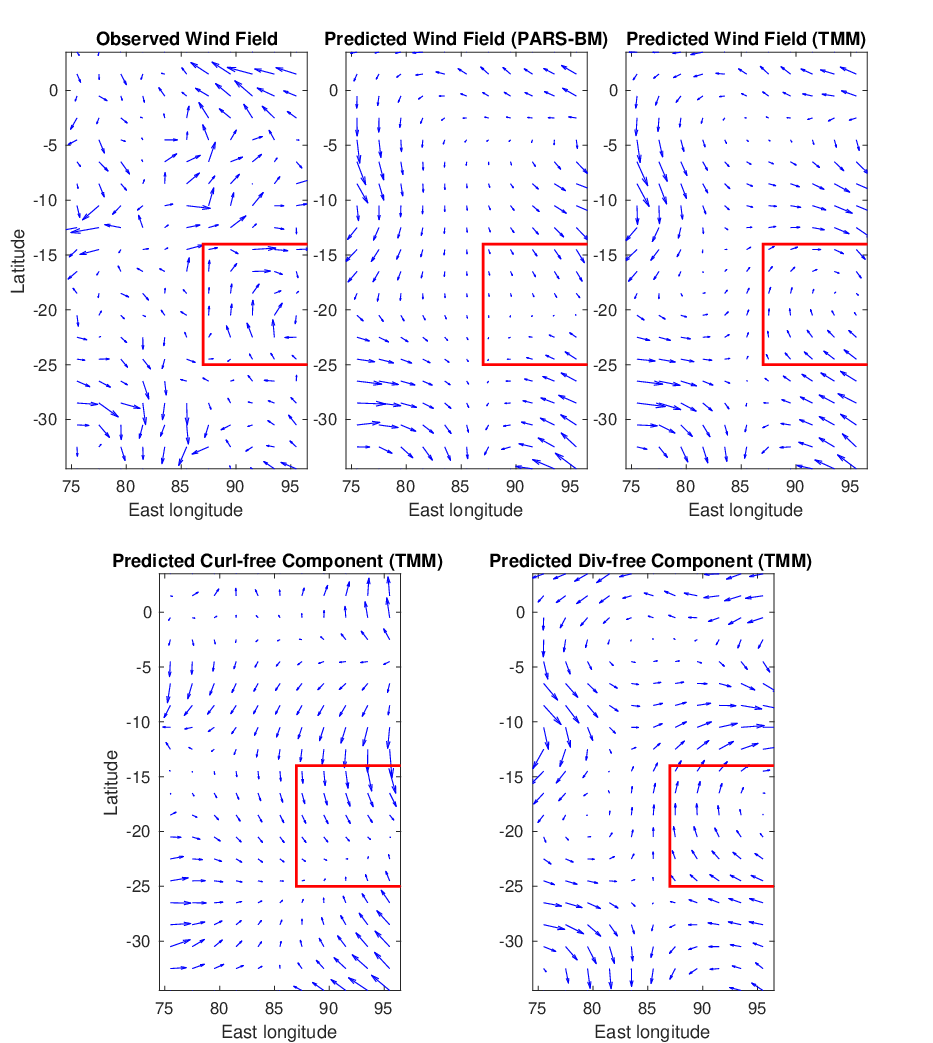
Finally, we compare the wind fields predicted by the two models with the observed one. The former are obtained by cokriging, which uses the locations outside the rectangular region to predict those within it, while the parameters are estimated based on the entire data set (see Table 1). Figure 10 shows the comparison among the wind fields within the rectangular region for January, 2000. It is not surprising that there are some discrepancies between the predicted and observed wind fields. Nonetheless, the predicted wind field by the TMM captures the rotational motion within the marked rectangle, which is missed by the PARS-BM.

5 Discussion

We have introduced a general framework to construct models for tangential vector fields on the unit sphere, using the surface gradient or the surface curl operator. Under this framework, we have presented a new class of parametric models, named Tangent Matérn Model, which is derived by using a bivariate Matérn model as the underlying potential field. Unlike most parametric models for vector fields that do not impose specific physical constraints, our model is directly motivated by the celebrated Helmholtz-Hodge decomposition, in which a tangential vector field is naturally decomposed into the sum of a curl-free and a divergence-free components. These two components carry important scientific meanings for describing the phenomena within the context of naturally occurring vector fields such as surface wind fields, oceanic currents, etc.

We have compared the Tangent Matérn Model with the parsimonious bivariate Matérn model on a QuikSCAT ocean surface wind velocity data set in terms of model fitting and spatial prediction. We focused on modeling the small-scale component, where the large-scale spatio-temporal component was subtracted using empirical orthogonal functions. In the comparison, our model captured the negative covariances and the rotational flow of the wind field, while the parsimonious bivariate Matérn model did not. As a result, the prediction error produced by our model was significantly smaller than that by the parsimonious bivariate Matérn model. This demonstrates the importance of incorporating these physical characteristics into the models for terrestrial physical processes.

A limitation of the Tangent Matérn Model is the assumption of isotropy for the underlying potential field. This isotropy assumption leads to Proposition 1, in which the co-located cross-covariance function is constant over the sphere, and in particular, $\mbox{Corr}\left(u(\textbf{s}),v(\textbf{s})\right)=0$ . Nonetheless, we can extend the model using an anisotropic underlying potential field, such as non-stationary bivariate Matérn models with spatially varying parameters (Kleiber and Nychka,, 2012; Jun,, 2014). The spatially varying parameters can be modeled by parametric functions of spherical harmonics (Bolin and Lindgren,, 2011) or covariates observed together with the vector field (Risser and Calder,, 2015). This remains a topic of future research.

Proposition 2 reveals the connection of our model with the models of Jun, (2011); Jun, (2014); Jun and Stein, (2008), although they are derived from different perspectives. Also, as demonstrated by Proposition 2, the tangential vector field that follows our model is axially symmetric when represented in the spherical coordinate system. Thus, this result enables fast computation for large data sets when the observations are on a regular grid. For example, on average, it takes approximately $8$ hours (on a machine with a 2.60GHz Intel Xeon E5-2690 v3 processor) to estimate the parameters when the sample size is as large as $5000$ . For irregularly spaced observations, apart from the method of covariance tapering mentioned in Section 2.4, a multi-resolution model constructed by the Wendland radial basis functions can also be used to represent or approximate the underlying potential field with a Matérn or a more complicated covariance structure (Nychka et al.,, 2015). Since the key matrices involved in the computation are sparse, this model can be applied to large data sets.

Appendix

Appendix A: Notation and Definition

In this subsection, we describe some auxiliary notations and definitions that are helpful for understanding the construction and characteristics of tangential vector fields on the unit sphere.

\mathbf{Q}_{\mathbf{s}}=:\hat{\mathbf{r}}\times\mathbf{P}_{\mathbf{s}}=\left(\begin{matrix}0&-s_{3}&s_{2}\\ s_{3}&0&-s_{1}\\ -s_{2}&s_{1}&0\end{matrix}\right).

(18)

The surface gradient and the surface curl operators can be represented in the spherical coordinate system except at the two poles,

\nabla_{\mathbf{s}}^{*}f=\frac{\partial f}{\partial\theta}\hat{\bm{\theta}}+\frac{1}{\sin\theta}\frac{\partial f}{\partial\phi}\hat{\bm{\phi}},

and

L_{\mathbf{s}}^{*}f=\frac{\partial f}{\partial\theta}\hat{\bm{\phi}}-\frac{1}{\sin\theta}\frac{\partial f}{\partial\phi}\hat{\bm{\theta}}.

Let $X(\mathbf{s})$ denote a scalar random field on a spherical shell $S_{\epsilon}$ , where $(\Omega,\mathcal{F},\mathbb{P})$ is the underlying probability space. The partial derivative of $X(\mathbf{s})$ in quadratic mean along the $i$ -th coordinate direction is defined as a random process $D_{\mathrm{qm}}^{(i)}X(\mathbf{s})$ such that

\mathbb{E}\left(\frac{X(\mathbf{s}+h\mathbf{e}_{i})-X(\mathbf{s})}{h}-D_{\mathrm{qm}}^{(i)}X(\mathbf{s})\right)^{2}\rightarrow 0\qquad\mbox{as}~h\rightarrow 0,

where $\mathbf{e}_{i}$ is the unit vector in $\mathbb{R}^{3}$ with the $i$ -th element one and zeros elsewhere. The sample partial derivatives of $X(\mathbf{s})$ , $D^{(i)}X(\mathbf{s}),i=1,2,3$ , are defined as the usual partial derivatives of $X(\mathbf{s},\omega)$ for any fixed $\omega\in\Omega$ . A random field $\widetilde{X}$ is said to be a $\mathbb{P}-$ a.e. sample continuously differentiable version of $X$ if the following hold:

(i)

For any $\mathbf{s}\in S_{\epsilon}$ , $\mathbb{P}\left(\widetilde{X}(\mathbf{s})=X(\mathbf{s})\right)=1$ .
(ii)

There exists $\Omega_{0}\subset\Omega$ with $\mathbb{P}(\Omega_{0})=1$ such that $\widetilde{X}(\mathbf{s},\omega)$ is continuously differentiable on $S_{\epsilon}$ for any $\omega\in\Omega_{0}$ .

A random tangential vector field on $\mathbb{S}^{2}$ is said to be curl-free or divergence-free if its sample paths are curl-free or divergence-free $\mathbb{P}-$ a.e.

Appendix B: Proof of Theorem 1

We first verify (1), and then (2) can be derived similarly. Since $D^{(i)}\widetilde{Z}(\mathbf{s})=D_{\mathrm{qm}}^{(i)}Z(\mathbf{s})$ $\mathbb{P}-$ a.e., $\mathbf{Y}_{\mathrm{curl},Z}(\mathbf{s})=\mathbf{P}_{\mathbf{s}}\nabla_{\mathbf{s},\mathrm{qm}}Z(\mathbf{s})$ $\mathbb{P}-$ a.e., where $\nabla_{\mathbf{s},\mathrm{qm}}$ is the usual gradient on $\mathbb{R}^{3}$ defined in the sense of quadratic mean. Thus,

$\displaystyle\mathbf{C}_{\mathrm{curl},Z}(\mathbf{s},\mathbf{t})$	$\displaystyle=$	$\displaystyle\mathbf{P}_{\mathbf{s}}\mathrm{Cov}\left(\nabla_{\mathbf{s},\mathrm{qm}}Z(\mathbf{s}),\nabla_{\mathbf{t},\mathrm{qm}}Z(\mathbf{t})\right)\mathbf{P}_{\mathbf{t}}^{\rm T}$
	$\displaystyle=$	$\displaystyle\mathbf{P}_{\mathbf{s}}\left[\mathrm{Cov}\left(D_{\mathrm{qm}}^{(i)}Z(\mathbf{s}),D_{\mathrm{qm}}^{(j)}Z(\mathbf{t})\right)\right]_{1\leq i,j\leq 3}\mathbf{P}_{\mathbf{t}}^{\rm T}$
	$\displaystyle=$	$\displaystyle\mathbf{P}_{\mathbf{s}}\left[\frac{\partial^{2}C}{\partial s_{i}\partial t_{j}}(\mathbf{s}-\mathbf{t})\right]_{1\leq i,j\leq 3}\mathbf{P}_{\mathbf{t}}^{\rm T}\qquad\mbox{by condition {A2}}$
	$\displaystyle=$	$\displaystyle-\mathbf{P}_{\mathbf{s}}\left[\frac{\partial^{2}C}{\partial h_{i}\partial h_{j}}(\mathbf{h})\right]_{1\leq i,j\leq 3}\bigg\|_{\mathbf{h}=\mathbf{s}-\mathbf{t}}\mathbf{P}_{\mathbf{t}}^{\rm T}$
	$\displaystyle=$	$\displaystyle-\mathbf{P}_{\mathbf{s}}\nabla_{\mathbf{h}}\nabla_{\mathbf{h}}^{\rm T}C(\mathbf{h})\bigg\|_{\mathbf{h}=\mathbf{s}-\mathbf{t}}\mathbf{P}_{\mathbf{t}}^{\rm T}.$

Appendix C: Proof that $\nu>1$ is necessary and sufficient

First, $\nu>1$ is necessary since the underlying potential field $Z(\mathbf{s})$ is required to be differentiable in quadratic mean. Second, we shall show the sufficiency. With $\nu>1$ and its Gaussianity, the sample paths of $Z$ are continuously differentiable $\mathbb{P}-$ a.e. (Handcock and Wallis,, 1994). Moreover, $Z$ has partial derivatives in quadratic mean. They imply that $\left(Z(\mathbf{s}+h\mathbf{e}_{i})-Z(\mathbf{s})\right)/h$ converges to $D_{\mathrm{qm}}^{(i)}Z(\mathbf{s})$ in $L_{2}$ (and in probability), and converges to $D^{(i)}Z(\mathbf{s})$ almost everywhere (and in probability). By the uniqueness of convergence in probability, $D_{\mathrm{qm}}^{(i)}Z(\mathbf{s})=D^{(i)}Z(\mathbf{s})$ $\mathbb{P}-$ a.e. Thus, we can choose $Z$ as $\widetilde{Z}$ so that condition A1 is satisfied. Jun and Stein, (2007) pointed out that the Matérn model (3) is twice continuously differentiable and $M^{\prime}(0;\nu,a)=0$ . Then $C_{1}(\lVert\mathbf{h}\rVert)$ is also twice continuously differentiable when $\lVert\mathbf{h}\rVert>0$ . It can be shown by definition that

\frac{\partial C_{1}(\lVert\mathbf{h}\rVert)}{\partial h_{i}}=\begin{cases}C^{\prime}_{1}(\lVert\mathbf{h}\rVert)\frac{h_{i}}{\lVert\mathbf{h}\rVert}&\mbox{if }\mathbf{h}\neq\mathbf{0}\\ 0&\mbox{if }\mathbf{h}=\mathbf{0}.\end{cases}

Based on the first derivatives, we can also show by definition that

\frac{\partial^{2}C_{1}(\lVert\mathbf{h}\rVert)}{\partial h_{i}\partial h_{j}}\bigg|_{\mathbf{h}=\mathbf{0}}=\begin{cases}0&\mbox{if }i\neq j\\ C_{1}^{\prime\prime}(0)&\mbox{if }i=j.\end{cases}

This is equivalent to

\nabla_{\mathbf{h}}\nabla_{\mathbf{h}}^{\rm T}C_{1}(\lVert\mathbf{h}\rVert)\bigg|_{\mathbf{h}=\mathbf{0}}=F(0)\mathbf{I}_{3}.

Together with

\lim_{\mathbf{h}\to\mathbf{0}}\nabla_{\mathbf{h}}\nabla_{\mathbf{h}}^{\rm T}C_{1}(\lVert\mathbf{h}\rVert)\bigg|_{\mathbf{h}\neq\mathbf{0}}=\lim_{\mathbf{h}\to\mathbf{0}}F(\lVert\mathbf{h}\rVert)\mathbf{I}_{3}+G(\lVert\mathbf{h}\rVert)\mathbf{h}\mathbf{h}^{\rm T}=F(0)\mathbf{I}_{3},

it implies that $C_{1}(\lVert\mathbf{h}\rVert)$ is twice continuously differentiable at $\mathbf{h}=\mathbf{0}$ . Thus, condition A2 is satisfied.

Appendix D: Isotropic $Z(\mathbf{s})$

Since $C_{1}(\lVert\mathbf{h}\rVert)$ is twice continuously differentiable when $h_{1}\geq 0$ and $h_{2}=h_{3}=0$ , $C_{1}(r)$ is also twice continuously differentiable. Moreover, the fact that $C_{1}(\lVert\mathbf{h}\rVert)$ is continuously differentiable at $\mathbf{h}=\mathbf{0}$ implies that $C_{1}^{\prime}(0)=0$ . Then we have

\nabla_{\mathbf{h}}\nabla_{\mathbf{h}}^{\rm T}C_{1}(\lVert\mathbf{h}\rVert)=\begin{cases}F(\lVert\mathbf{h}\rVert)\mathbf{I}_{3}+G(\lVert\mathbf{h}\rVert)\mathbf{h}\mathbf{h}^{\rm T}&\mbox{if }\mathbf{h}\neq\mathbf{0}\\ F(0)\mathbf{I}_{3}&\mbox{if }\mathbf{h}=\mathbf{0},\end{cases}

(19)

where

F(r)=\begin{cases}\frac{1}{r}C_{1}^{\prime}(r)&\mbox{if }r>0\\ C_{1}^{\prime\prime}(0)&\mbox{if }r=0,\end{cases}

(20)

and

G(r)=\frac{1}{r}\left(\frac{1}{r}C_{1}^{\prime}(r)\right)^{\prime}\quad\mbox{if }r>0.

(21)

Here the value of $\nabla_{\mathbf{h}}\nabla_{\mathbf{h}}^{\rm T}C_{1}(\lVert\mathbf{h}\rVert)$ at $\mathbf{h}=\mathbf{0}$ is obtained by

\lim_{\mathbf{h}\to\mathbf{0}}F(\lVert\mathbf{h}\rVert)\mathbf{I}_{3}+G(\lVert\mathbf{h}\rVert)\mathbf{h}\mathbf{h}^{\rm T}=F(0)\mathbf{I}_{3}.

When $C_{1}$ is chosen as the Matérn model, we have the explicit expressions of $F$ and $G$ as

F_{\textrm{Mat}}(r;\nu,a)=\begin{cases}-\frac{2^{1-\nu}}{\Gamma(\nu)}a^{2}(ar)^{\nu-1}K_{\nu-1}(ar)&\mbox{if }r>0\\ -\frac{a^{2}}{2(\nu-1)}&\mbox{if }r=0,\end{cases}

(22)

and

G_{\textrm{Mat}}(r;\nu,a)=\frac{2^{1-\nu}}{\Gamma(\nu)}a^{4}(ar)^{\nu-2}K_{\nu-2}(ar)\quad\mbox{if }r>0,

(23)

where $\nu>1$ .

Appendix E: Proof of Proposition 1

Let $\mathbf{Y}(\mathbf{s})=(Y_{1}(\mathbf{s}),Y_{2}(\mathbf{s}),Y_{3}(\mathbf{s}))^{\rm T}$ denote a tangential vector field in Cartesian coordinates with cross-covariance function $\mathbf{C}_{\mathrm{tan},\mathbf{Z}}(\mathbf{s},\mathbf{t})$ . It can be converted to the canonical coordinates $(\hat{\mathbf{u}},\hat{\mathbf{v}})$ by the transformation

\mathbf{V}(\mathbf{s})\equiv(u(\mathbf{s}),v(\mathbf{s}))^{\rm T}=\mathbf{T}_{\mathbf{s}}\mathbf{Y}(\mathbf{s}),

where

\mathbf{T}_{\mathbf{s}}=\left(\begin{matrix}-\sin\phi_{\mathbf{s}}&\cos\phi_{\mathbf{s}}&0\\ -\cos\theta_{\mathbf{s}}\cos\phi_{\mathbf{s}}&-\cos\theta_{\mathbf{s}}\sin\phi_{\mathbf{s}}&\sin\theta_{\mathbf{s}}\end{matrix}\right).

Then the cross-covariance function of $\mathbf{V}$ is

\mathbf{C}_{\mathbf{V}}(\mathbf{s},\mathbf{t})=\mathbf{T}_{\mathbf{s}}\mathbf{C}_{\mathrm{tan},\mathbf{Z}}(\mathbf{s},\mathbf{t})\mathbf{T}_{\mathbf{t}}^{\rm T}.

Notice that

\mathbf{T}_{\mathbf{s}}\mathbf{P}_{\mathbf{s}}=\left(\begin{matrix}-\sin\phi_{\mathbf{s}}&\cos\phi_{\mathbf{s}}&0\\ -\cos\theta_{\mathbf{s}}\cos\phi_{\mathbf{s}}&-\cos\theta_{\mathbf{s}}\sin\phi_{\mathbf{s}}&\sin\theta_{\mathbf{s}}\end{matrix}\right),

and

\mathbf{T}_{\mathbf{s}}\mathbf{Q}_{\mathbf{s}}=\left(\begin{matrix}\cos\theta_{\mathbf{s}}\cos\phi_{\mathbf{s}}&\cos\theta_{\mathbf{s}}\sin\phi_{\mathbf{s}}&-\sin\theta_{\mathbf{s}}\\ -\sin\phi_{\mathbf{s}}&\cos\phi_{\mathbf{s}}&0\end{matrix}\right).

Plugging in them to the expression of $\mathbf{C}_{\mathrm{tan},\mathbf{Z}}(\mathbf{s},\mathbf{t})$ , we have

\mathbf{C}_{\mathbf{V}}(\mathbf{s},\mathbf{s})=-\left[\sigma_{1}^{2}F_{\textrm{Mat}}(0;\nu_{1},a)+\sigma_{2}^{2}F_{\textrm{Mat}}(0;\nu_{2},a)\right]\mathbf{I}_{2},

which is constant with respect to $\mathbf{s}$ .

By making use of (8) and (9), we can intuitively understand the conclusion that the co-located correlation between $u$ and $v$ has to be zero. Since $Z_{1}$ is isotropic, the change rates of the field at the same location along latitudinal and longitudinal directions are uncorrelated, i.e., $\mbox{Cov}(\partial Z_{1}/\partial\phi,\partial Z_{1}/\partial\theta)=0$ (Adler and Taylor,, 2009, page 116, (5.7.3)). Similarly, the same holds for $Z_{2}$ . Moreover, the cross-covariance between $Z_{1}$ and $Z_{2}$ is also isotropic. Due to the curvature of the sphere, for $Z_{1}$ and $Z_{2}$ , the covariance of the change rates along latitudinal direction equals the covariance of the change rates along longitudinal direction multiplied by $\sin^{2}\theta$ , i.e., $\mbox{Cov}(\partial Z_{1}/\partial\phi,\partial Z_{2}/\partial\phi)=\mbox{Cov}(\partial Z_{2}/\partial\theta,\partial Z_{1}/\partial\theta)\sin^{2}\theta$ .

Appendix F: Proof of Proposition 2

According to the construction of the TMM, for any $(\theta,\phi)$ except at the two poles,

$\displaystyle u(\theta,\phi)\hat{\mathbf{u}}+v(\theta,\phi)\hat{\mathbf{v}}$	$\displaystyle=$	$\displaystyle\nabla^{}_{\mathbf{s}}\widetilde{Z}_{1}(\mathbf{s})+L^{}_{\mathbf{s}}\widetilde{Z}_{2}(\mathbf{s})\qquad\mathbb{P-}\mbox{a.e.}$
	$\displaystyle=$	$\displaystyle\left(\frac{1}{\sin{\theta}}\frac{\partial{\widetilde{Z}_{1}}}{\partial\phi}+\frac{\partial{\widetilde{Z}_{2}}}{\partial\theta}\right)\hat{\bm{\phi}}-\left(\frac{1}{\sin{\theta}}\frac{\partial{\widetilde{Z}_{2}}}{\partial\phi}-\frac{\partial{\widetilde{Z}_{1}}}{\partial\theta}\right)\hat{\bm{\theta}}$
	$\displaystyle=$	$\displaystyle\left(\frac{1}{\sin{\theta}}\frac{\partial{\widetilde{Z}_{1}}}{\partial\phi}+\frac{\partial{\widetilde{Z}_{2}}}{\partial\theta}\right)\hat{\mathbf{u}}+\left(\frac{1}{\sin{\theta}}\frac{\partial{\widetilde{Z}_{2}}}{\partial\phi}-\frac{\partial{\widetilde{Z}_{1}}}{\partial\theta}\right)\hat{\mathbf{v}}.$

Thus,

u(\theta,\phi)=\frac{1}{\sin{\theta}}\frac{\partial{\widetilde{Z}_{1}}}{\partial\phi}+\frac{\partial{\widetilde{Z}_{2}}}{\partial\theta}\qquad\mathbb{P-}\mbox{a.e.},

and

v(\theta,\phi)=\frac{1}{\sin{\theta}}\frac{\partial{\widetilde{Z}_{2}}}{\partial\phi}-\frac{\partial{\widetilde{Z}_{1}}}{\partial\theta}\qquad\mathbb{P-}\mbox{a.e.}

By condition A1 and the chain rule for partial derivatives in quadratic mean (Potthoff,, 2010, Theorem 2.13), (8) and (9) follow.

We have assumed that the cross-covariance function of $(Z_{1}(\mathbf{s}),Z_{2}(\mathbf{s}))^{\rm T}$ (restricted on $\mathbb{S}^{2}$ ) only depends on the chordal distance, which is a function of $\theta_{1},\theta_{2}$ and $\phi_{1}-\phi_{2}$ . Moreover, the coefficients of the partial derivatives are independent of longitude. Using the same argument as Jun and Stein, (2008), we conclude that $u$ and $v$ are axially symmetric both marginally and jointly.

References

Adler and Taylor, (2009) Adler, R. J. and Taylor, J. E. (2009). Random fields and geometry. Springer Science & Business Media.
Apanasovich et al., (2012) Apanasovich, T. V., Genton, M. G., and Sun, Y. (2012). A valid Matérn class of cross-covariance functions for multivariate random fields with any number of components. Journal of the American Statistical Association, 107(497):180–193.
Atlas et al., (2001) Atlas, R., Hoffman, R. N., Leidner, S. M., Sienkiewicz, J., Yu, T.-W., Bloom, S. C., Brin, E., Ardizzone, J., Terry, J., Bungato, D., and Jusem, J. C. (2001). The effects of marine winds from scatterometer data on weather analysis and forecasting. Bulletin of the American Meteorological Society, 82:1965–1990.
Bevilacqua et al., (2015) Bevilacqua, M., Fassò, A., Gaetan, C., Porcu, E., and Velandia, D. (2015). Covariance tapering for multivariate gaussian random fields estimation. Statistical Methods & Applications, pages 1–17.
Bijlsma et al., (1986) Bijlsma, S., Hafkenscheid, L., and Lynch, P. (1986). Computation of the streamfunction and velocity potential and reconstruction of the wind field. Monthly weather review, 114(8):1547–1551.
Bolin and Lindgren, (2011) Bolin, D. and Lindgren, F. (2011). Spatial models generated by nested stochastic partial differential equations, with an application to global ozone mapping. The Annals of Applied Statistics, 5(1):523–550.
Bourgault and Marcotte, (1991) Bourgault, G. and Marcotte, D. (1991). Multivariable variogram and its application to the linear model of coregionalization. Mathematical Geology, 23(7):899–928.
Brennan et al., (2009) Brennan, M. J., Hennon, C. C., and Knabb, R. D. (2009). The operational use of QuikSCAT ocean surface vector winds at the National Hurricane Center. Weather and Forecasting, 24:621–645.
Constantinescu and Anitescu, (2013) Constantinescu, E. M. and Anitescu, M. (2013). Physics-based covariance models for Gaussian processes with multiple outputs. International Journal for Uncertainty Quantification, 3(1).
Cornford, (1998) Cornford, D. (1998). Flexible Gaussian process wind field models. Technical Report NCRG/98/017, Neural Computing Research Group, Aston University, Birmingham.
Cornford et al., (2004) Cornford, D., Csató, L., Evans, D. J., and Opper, M. (2004). Bayesian analysis of the scatterometer wind retrieval inverse problem: some new approaches. Journal of the Royal Statistical Society: Series B (Statistical Methodology), 66(3):609–626.
Cressie and Huang, (1999) Cressie, N. and Huang, H.-C. (1999). Classes of nonseparable, spatio-temporal stationary covariance functions. Journal of the American Statistical Association, 94(448):1330–1339.
Cressie and Wikle, (2011) Cressie, N. and Wikle, C. K. (2011). Statistics for spatio-temporal data. John Wiley & Sons.
Daley, (1991) Daley, R. (1991). Atmospheric data analysis. Cambridge: Cambridge University Press.
Foley and Fuentes, (2008) Foley, K. and Fuentes, M. (2008). A statistical framework to combine multivariate spatial data and physical models for hurricane surface wind prediction. Journal of Agricultural, Biological, and Environmental Statistics, 13(1):37–59.
Freeden and Schreiner, (2009) Freeden, W. and Schreiner, M. (2009). Spherical functions of mathematical geosciences: a scalar, vectorial, and tensorial setup. Advances in Geophysical and Environmental Mechanics and Mathematics. Springer-Verlag Berlin Heidelberg.
Furrer et al., (2006) Furrer, R., Genton, M. G., and Nychka, D. (2006). Covariance tapering for interpolation of large spatial datasets. Journal of Computational and Graphical Statistics, 15(3):502–523.
Fuselier and Wright, (2009) Fuselier, E. J. and Wright, G. B. (2009). Stability and error estimates for vector field interpolation and decomposition on the sphere with RBFs. SIAM Journal on Numerical Analysis, 47(5):3213–3239.
Gelfand et al., (2004) Gelfand, A. E., Schmidt, A. M., Banerjee, S., and Sirmans, C. F. (2004). Nonstationary multivariate process modeling through spatially varying coregionalization. Test, 13(2):263–312.
Gneiting et al., (2010) Gneiting, T., Kleiber, W., and Schlather, M. (2010). Matérn cross-covariance functions for multivariate random fields. Journal of the American Statistical Association, 105(491):1167–1177.
Górski et al., (2005) Górski, K. M., Hivon, E., Banday, A. J., Wandelt, B. D., Hansen, F. K., Reinecke, M., and Bartelmann, M. (2005). HEALPix: A framework for high-resolution discretization and fast analysis of data distributed on the sphere. The Astrophysical Journal, 622(2):759.
Goulard and Voltz, (1992) Goulard, M. and Voltz, M. (1992). Linear coregionalization model: Tools for estimation and choice of cross-variogram matrix. Mathematical Geology, 24(3):269–286.
Guinness and Fuentes, (2015) Guinness, J. and Fuentes, M. (2015). Isotropic covariance functions on spherese : some properties and modeling considerations. Journal of Multivariate Analysis. To appear.
Handcock and Wallis, (1994) Handcock, M. S. and Wallis, J. R. (1994). An approach to statistical spatial-temporal modeling of meteorological fields. Journal of the American Statistical Association, 89(426):368–378.
Hitczenko and Stein, (2012) Hitczenko, M. and Stein, M. L. (2012). Some theory for anisotropic processes on the sphere. Statistical Methodology, 9:211–227.
Holton, (2004) Holton, J. R. (2004). An introduction to dynamic meteorology. International geophysics series. Elsevier Academic Press, Amsterdam, Boston, Heidelberg.
Horowitz, (2001) Horowitz, J. L. (2001). The bootstrap. Handbook of econometrics, 5:3159–3228.
Hsu et al., (2012) Hsu, N.-J., Chang, Y.-M., and Huang, H.-C. (2012). A group lasso approach for non-stationary spatial–temporal covariance estimation. Environmetrics, 23(1):12–23.
Jones, (1963) Jones, R. H. (1963). Stochastic processes on a sphere. Annals of Mathematical Statistics, 34(1):213–218.
Jun, (2011) Jun, M. (2011). Non-stationary cross-covariance models for multivariate processes on a globe. Scandinavian Journal of Statistics, 38(4):726–747.
Jun, (2014) Jun, M. (2014). Matérn-based nonstationary cross-covariance models for global processes. Journal of Multivariate Analysis, 128:134–146.
Jun and Stein, (2007) Jun, M. and Stein, M. L. (2007). An approach to producing space-time covariance functions on spheres. Technometrics, 49(4):468–479.
Jun and Stein, (2008) Jun, M. and Stein, M. L. (2008). Nonstationary covariance models for global data. The Annals of Applied Statistics, 2(4):1271–1289.
Kadri-Harouna and Perrier, (2012) Kadri-Harouna, S. and Perrier, V. (2012). Helmholtz-Hodge decomposition on $[0,1]^{d}$ by divergence-free and curl-free wavelets. In Boissonnat, J.-D., Chenin, P., Cohen, A., Gout, C., Lyche, T., Mazure, M.-L., and Schumaker, L., editors, Curves and Surfaces, volume 6920 of Lecture Notes in Computer Science, pages 311–329. Springer Berlin Heidelberg.
Kaufman et al., (2008) Kaufman, C. G., Schervish, M. J., and Nychka, D. W. (2008). Covariance tapering for likelihood-based estimation in large spatial data sets. Journal of the American Statistical Association, 103(484):1545–1555.
Kaufman and Shaby, (2013) Kaufman, C. G. and Shaby, B. A. (2013). The role of the range parameter for estimation and prediction in geostatistics. Biometrika, 100(2):473–484.
Kleiber and Nychka, (2012) Kleiber, W. and Nychka, D. (2012). Nonstationary modeling for multivariate spatial processes. Journal of Multivariate Analysis, 112:76–91.
Marinucci and Peccati, (2011) Marinucci, D. and Peccati, G. (2011). Random Fields on the Sphere: Representation, Limit Theorems and Cosmological Applications, volume 389 of London Mathematical Society Lecture Note Series. Cambridge University Press.
Matsuo et al., (2011) Matsuo, T., Nychka, D. W., and Paul, D. (2011). Nonstationary covariance modeling for incomplete data: Monte carlo em approach. Computational Statistics & Data Analysis, 55(6):2059–2073.
Myers, (1982) Myers, D. E. (1982). Matrix formulation of co-kriging. Journal of the International Association for Mathematical Geology, 14(3):249–257.
Narcowich et al., (2007) Narcowich, F. J., Ward, J. D., and Wright, G. B. (2007). Divergence-free RBFs on surfaces. Journal of Fourier Analysis and Applications, 13(6):643–663.
Nychka et al., (2015) Nychka, D., Bandyopadhyay, S., Hammerling, D., Lindgren, F., and Sain, S. (2015). A multiresolution gaussian process model for the analysis of large spatial datasets. Journal of Computational and Graphical Statistics, 24(2):579–599.
Nychka et al., (2002) Nychka, D., Wikle, C., and Royle, J. A. (2002). Multiresolution models for nonstationary spatial covariance functions. Statistical Modelling, 2(4):315–331.
Pan et al., (2001) Pan, J., Yan, X.-H., Zheng, Q., and Liu, W. T. (2001). Vector empirical orthogonal function modes of the ocean surface wind variability derived from satellite scatterometer data. Geophysical Research Letters, 28(20):3951–3954.
Pan et al., (2003) Pan, J., Yan, X.-H., Zheng, Q., Liu, W. T., and Klemas, V. V. (2003). Interpretation of scatterometer ocean surface wind vector EOFs over the northwestern Pacific. Remote sensing of environment, 84(1):53–68.
Park, (2001) Park, C. C. (2001). The environment: principles and applications. Psychology Press.
Piolle and Bentamy, (2002) Piolle, J.-F. and Bentamy, A. (2002). QuikSCAT scatterometer mean wind field products user manual. Ifremer, Department of Oceanography from Space, Ref.: C2-MUT-W-04-IF, Version 1.0, May 2002.
Potthoff, (2010) Potthoff, J. (2010). Sample properties of random fields III: Differentiability. Communications on Stochastic Analysis, 4(3):335–353.
Reich and Fuentes, (2007) Reich, B. J. and Fuentes, M. (2007). A multivariate semiparametric bayesian spatial modeling framework for hurricane surface wind fields. The Annals of Applied Statistics, 1(1):249–264.
Richmond and Kamide, (1988) Richmond, A. D. and Kamide, Y. (1988). Mapping electrodynamic features of the high-latitude ionosphere from localized observations: Technique. Journal of Geophysical Research: Space Physics, 93(A6):5741–5759.
Risser and Calder, (2015) Risser, M. D. and Calder, C. A. (2015). Regression-based covariance functions for nonstationary spatial modeling. Environmetrics, 26(4):284–297.
Sabaka et al., (2010) Sabaka, T. J., Hulot, G., and Olsen, N. (2010). Mathematical properties relevant to geomagnetic field modeling. In Freeden, W., Nashed, M. Z., and Sonar, T., editors, Handbook of Geomathematics, pages 503–538. Springer Berlin Heidelberg.
Scheuerer and Schlather, (2012) Scheuerer, M. and Schlather, M. (2012). Covariance models for divergence-free and curl-free random vector fields. Stochastic Models, 28(3):433–451.
Schlather et al., (2015) Schlather, M., Malinowski, A., Menck, P. J., Oesting, M., and Strokorb, K. (2015). Analysis, simulation and prediction of multivariate random fields with package RandomFields. Journal of Statistical Software, 63(8):1–25.
Shukla and Saha, (1974) Shukla, J. and Saha, K. (1974). Computation of non-divergent streamfunction and irrotational velocity potential from the observed winds. Monthly weather review, 102(6):419–425.
Stein, (2007) Stein, M. L. (2007). Spatial variation of total column ozone on a global scale. The Annals of Applied Statistics, pages 191–210.
Ver Hoef and Cressie, (1993) Ver Hoef, J. M. and Cressie, N. (1993). Multivariable spatial prediction. Mathematical Geology, 25(2):219–240.
Wikle and Cressie, (1999) Wikle, C. K. and Cressie, N. (1999). A dimension-reduced approach to space-time Kalman filtering. Biometrika, 86(4):815–829.
Wikle et al., (2001) Wikle, C. K., Milliff, R. F., Nychka, D., and Berliner, L. M. (2001). Spatiotemporal hierarchical bayesian modeling tropical ocean surface winds. Journal of the American Statistical Association, 96(454):382–397.
Zhang, (2004) Zhang, H. (2004). Inconsistent estimation and asymptotically equal interpolations in model-based geostatistics. Journal of the American Statistical Association, 99(465):250–261.
Zhang et al., (2007) Zhang, Z., Beletsky, D., Schwab, D. J., and Stein, M. L. (2007). Assimilation of current measurements into a circulation model of Lake Michigan. Water resources research, 43(11).

Supplementary Materials for “Modeling Tangential Vector Fields on a Sphere”

S1: Implementation of the DFT for the cross-covariance matrix

Suppose the observations are on a regular grid on the sphere $\{(\theta_{i},\phi_{j}):i=1,\cdots,n_{\rm lat},j=1,\cdots,n_{\rm lon}\}$ , where $\theta$ and $\phi$ represent the co-latitude and the longitude, respectively. Besides, $\theta_{i}-\theta_{i-1}=(\theta_{n_{\rm lat}}-\theta_{1})/(n_{\rm lat}-1)$ and $\phi_{j}-\phi_{j-1}=2\pi/n_{\rm lon}$ , $\phi_{1}=0$ , $\phi_{n_{\rm lon}}=2\pi-2\pi/n_{\rm lon}$ . Denote the observations as $(Y_{1}(\theta_{i},\phi_{j}),Y_{2}(\theta_{i},\phi_{j}))^{\rm T},i=1,\cdots,n_{\rm lat},j=1,\cdots,n_{\rm lon}$ . We rearrange and stack them as $\left(\mathbf{Y}(\theta_{1})^{\rm T},\cdots,\mathbf{Y}(\theta_{n_{\rm lat}})^{\rm T}\right)^{\rm T}$ , where

\mathbf{Y}(\theta_{i})=\left(\mathbf{Y}_{1}(\theta_{i})^{\rm T},\mathbf{Y}_{2}(\theta_{i})^{\rm T}\right)^{\rm T}=\left(Y_{1}(\theta_{i},\phi_{1}),\cdots,Y_{1}(\theta_{i},\phi_{n_{\rm lon}}),Y_{2}(\theta_{i},\phi_{1}),\cdots,Y_{2}(\theta_{i},\phi_{n_{\rm lon}})\right)^{\rm T}.

Since the cross-covariance function of the random field $\mathbf{Y}$ is axially symmetric,

\mbox{Cov}\left(\mathbf{Y}(\theta_{i}),\mathbf{Y}(\theta_{j})\right)=\mathbb{E}\left(\mathbf{Y}(\theta_{i})\mathbf{Y}(\theta_{j})^{\rm T}\right)\\ =\left(\begin{matrix}\mathbb{E}\left(\mathbf{Y}_{1}(\theta_{i})\mathbf{Y}_{1}(\theta_{j})^{\rm T}\right)&\mathbb{E}\left(\mathbf{Y}_{1}(\theta_{i})\mathbf{Y}_{2}(\theta_{j})^{\rm T}\right)\\ \mathbb{E}\left(\mathbf{Y}_{2}(\theta_{i})\mathbf{Y}_{1}(\theta_{j})^{\rm T}\right)&\mathbb{E}\left(\mathbf{Y}_{2}(\theta_{i})\mathbf{Y}_{2}(\theta_{j})^{\rm T}\right)\\ \end{matrix}\right)\\ =\left(\begin{matrix}\left[C_{11}(\theta_{i},\theta_{j},\phi_{k}-\phi_{l})\right]_{1\leq k,l\leq n_{\rm lon}}&\left[C_{12}(\theta_{i},\theta_{j},\phi_{k}-\phi_{l})\right]_{1\leq k,l\leq n_{\rm lon}}\\ \left[C_{21}(\theta_{i},\theta_{j},\phi_{k}-\phi_{l})\right]_{1\leq k,l\leq n_{\rm lon}}&\left[C_{22}(\theta_{i},\theta_{j},\phi_{k}-\phi_{l})\right]_{1\leq k,l\leq n_{\rm lon}}\end{matrix}\right)=\left(\begin{matrix}\mathbf{C}_{11}(\theta_{i},\theta_{j})&\mathbf{C}_{12}(\theta_{i},\theta_{j})\\ \mathbf{C}_{21}(\theta_{i},\theta_{j})&\mathbf{C}_{22}(\theta_{i},\theta_{j})\end{matrix}\right),

where $\mathbf{C}_{\cdot\cdot}(\theta_{i},\theta_{j})$ are circulant matrices, which have the form (omitting the subscripts $\cdot\cdot$ )

\left(\begin{matrix}c_{0}&c_{n_{\rm lon}-1}&\cdots&c_{1}\\ c_{1}&c_{0}&\cdots&c_{2}\\ \vdots&\vdots&&\vdots\\ c_{n_{\rm lon}-1}&c_{n_{\rm lon}-2}&\cdots&c_{0}\end{matrix}\right).

A circulant matrix can be diagonalized by the DFT matrix

\mathbf{F}\mathbf{C}_{\cdot\cdot}(\theta_{i},\theta_{j})\mathbf{F}^{-1}=\bm{\Lambda}_{\cdot\cdot},

where

\mathbf{F}=\left(\begin{matrix}1&1&\cdots&1\\ 1&\omega^{1}&\cdots&\omega^{n_{\rm lon}-1}\\ 1&\omega^{2}&\cdots&\omega^{2(n_{\rm lon}-1)}\\ \vdots&\vdots&&\vdots\\ 1&\omega^{n_{\rm lon}-1}&\cdots&\omega^{(n_{\rm lon}-1)(n_{\rm lon}-1)}\end{matrix}\right),

and $\omega=\exp{(-2\pi i/n_{\rm lon})}$ . The diagonal matrix $\bm{\Lambda}_{\cdot\cdot}$ can be computed by

\bm{\Lambda}_{\cdot\cdot}=\mbox{diag}(\mathbf{F}\mathbf{c}_{\cdot\cdot}),

where $\mathbf{c}_{\cdot\cdot}=(c_{0},\cdots,c_{n_{\rm lon}-1})^{\rm T}$ . The observations are transformed accordingly

\mathbf{Y}(\theta_{i})=\left(\mathbf{Y}_{1}(\theta_{i})^{\rm T},\mathbf{Y}_{2}(\theta_{i})^{\rm T}\right)^{\rm T}\longrightarrow\left(\widetilde{\mathbf{Y}}_{1}(\theta_{i})^{\rm T},\widetilde{\mathbf{Y}}_{2}(\theta_{i})^{\rm T}\right)^{\rm T}=\left(\left(\mathbf{F}\mathbf{Y}_{1}(\theta_{i})\right)^{\rm T}/\sqrt{n_{\rm lon}},\left(\mathbf{F}\mathbf{Y}_{2}(\theta_{i})\right)^{\rm T}/\sqrt{n_{\rm lon}}\right)^{\rm T},

such that

\mathbb{E}\left(\widetilde{\mathbf{Y}}_{\cdot}(\theta_{i})\widetilde{\mathbf{Y}}_{\cdot}(\theta_{j})^{\rm H}\right)=\mathbf{F}\mathbb{E}\left(\mathbf{Y}_{\cdot}(\theta_{i})\mathbf{Y}_{\cdot}(\theta_{j})^{\rm T}\right)\mathbf{F}^{\rm H}/n_{\rm lon}\\ =\mathbf{F}\mathbb{E}\left(\mathbf{Y}_{\cdot}(\theta_{i})\mathbf{Y}_{\cdot}(\theta_{j})^{\rm T}\right)\mathbf{F}^{-1}=\bm{\Lambda}_{\cdot\cdot},

where $\cdot^{\rm H}$ represents the Hermitian transpose. We rearrange the order of the observations

\left(\widetilde{Y}_{1}(\theta_{1},\phi_{1}),\cdots,\widetilde{Y}_{1}(\theta_{n_{\rm lat}},\phi_{1}),\cdots,\widetilde{Y}_{1}(\theta_{1},\phi_{n_{\rm lon}}),\cdots,\widetilde{Y}_{1}(\theta_{n_{\rm lat}},\phi_{n_{\rm lon}}),\\ \widetilde{Y}_{2}(\theta_{1},\phi_{1}),\cdots,\widetilde{Y}_{2}(\theta_{n_{\rm lat}},\phi_{1}),\cdots,\widetilde{Y}_{2}(\theta_{1},\phi_{n_{\rm lon}}),\cdots,\widetilde{Y}_{2}(\theta_{n_{\rm lat}},\phi_{n_{\rm lon}})\right)^{\rm T}.

Then the corresponding cross-covariance matrix is

\bm{\Sigma}=\left(\begin{matrix}\bm{\Sigma}_{1}&\bm{\Sigma}_{12}\\ \bm{\Sigma}_{12}^{\rm H}&\bm{\Sigma}_{2}\end{matrix}\right),

where $\bm{\Sigma}_{1},\bm{\Sigma}_{12}$ and $\bm{\Sigma}_{2}$ are complex block diagonal matrices. The determinant of $\bm{\Sigma}$ can be computed by

\mbox{det}(\bm{\Sigma})=\mbox{det}(\bm{\Sigma}_{1}-\bm{\Sigma}_{12}\bm{\Sigma}_{2}^{-1}\bm{\Sigma}_{12}^{\rm H})\mbox{det}(\bm{\Sigma}_{2}),

and the inverse of $\bm{\Sigma}$ can be computed by

\bm{\Sigma}^{-1}=\left(\begin{matrix}(\bm{\Sigma}_{1}-\bm{\Sigma}_{12}\bm{\Sigma}_{2}^{-1}\bm{\Sigma}_{12}^{\rm H})^{-1}&-\bm{\Sigma}_{1}^{-1}\bm{\Sigma}_{12}(\bm{\Sigma}_{2}-\bm{\Sigma}_{12}^{\rm H}\bm{\Sigma}_{1}^{-1}\bm{\Sigma}_{12})^{-1}\\ (-\bm{\Sigma}_{1}^{-1}\bm{\Sigma}_{12}(\bm{\Sigma}_{2}-\bm{\Sigma}_{12}^{\rm H}\bm{\Sigma}_{1}^{-1}\bm{\Sigma}_{12})^{-1})^{\rm H}&(\bm{\Sigma}_{2}-\bm{\Sigma}_{12}^{\rm H}\bm{\Sigma}_{1}^{-1}\bm{\Sigma}_{12})^{-1}\end{matrix}\right),

where the inverses of $\bm{\Sigma}_{1}$ and $\bm{\Sigma}_{2}$ can be computed efficiently since they are both block diagonal matrices.

S2: Tangential vector fields derived from a full bivariate Matérn model

The underlying random field Z is assumed to follow a full bivariate Matérn model (Gneiting et al.,, 2010)

C_{ii}(\lVert\mathbf{h}\rVert)=\sigma_{i}^{2}M(\lVert\mathbf{h}\rVert;\nu_{i},a_{i})\qquad\mbox{for }i=1,2,

and

C_{12}(\lVert\mathbf{h}\rVert)=C_{21}(\lVert\mathbf{h}\rVert)=\rho_{12}\sigma_{1}\sigma_{2}M(\lVert\mathbf{h}\rVert;\nu_{12},a_{12}).

It is valid if and only if

\rho_{12}^{2}\leq\frac{\Gamma\left(\nu_{1}+\frac{d}{2}\right)}{\Gamma(\nu_{1})}\frac{\Gamma\left(\nu_{2}+\frac{d}{2}\right)}{\Gamma(\nu_{2})}\frac{\Gamma(\nu_{12})^{2}}{\Gamma\left(\nu_{12}+\frac{d}{2}\right)^{2}}\frac{a_{1}^{2\nu_{1}}a_{2}^{2\nu_{2}}}{a_{12}^{4\nu_{12}}}\inf\limits_{t\geq 0}\frac{(a_{12}^{2}+t^{2})^{2\nu_{12}+d}}{(a_{1}^{2}+t^{2})^{\nu_{1}+(d/2)}(a_{2}^{2}+t^{2})^{\nu_{2}+(d/2)}}.

(S1)

Condition (S1) implies that if $\nu_{12}<\frac{1}{2}(\nu_{1}+\nu_{2})$ , $\rho_{12}$ has to be zero, i.e., the two Cartesian components of Z are independent. Thus, we are mainly interested in the case when $\nu_{12}\geq\frac{1}{2}(\nu_{1}+\nu_{2})$ .

The derived cross-covariance function of $\mathbf{Y}_{\mathrm{tan},\mathbf{Z}}(\mathbf{s})$ is

			$\displaystyle\mathbf{C}_{\mathrm{tan},\mathbf{Z}}(\mathbf{s},\mathbf{t})$
		$\displaystyle=$	$\displaystyle-\left(\begin{matrix}\sigma_{1}\mathbf{P}_{\mathbf{s}}&\sigma_{2}\mathbf{Q}_{\mathbf{s}}\end{matrix}\right)\left(\begin{matrix}\mathbf{K}(\mathbf{h};\nu_{1},a_{1})&\rho_{12}\mathbf{K}(\mathbf{h};\nu_{12},a_{12})\\ \rho_{12}\mathbf{K}(\mathbf{h};\nu_{12},a_{12})&\mathbf{K}(\mathbf{h};\nu_{2},a_{2})\end{matrix}\right)\left(\begin{matrix}\sigma_{1}\mathbf{P}_{\mathbf{t}}^{\rm T}\\ \sigma_{2}\mathbf{Q}_{\mathbf{t}}^{\rm T}\end{matrix}\right),$

where $\nu_{1},\nu_{2}>1$ .

S3: Accuracy of parameter estimation on irregular grids

To investigate the accuracy of parameter estimation on irregular grids, we conduct some smaller scale experiments (due to the computational cost). Specifically, we generate $100$ realizations with

\bm{\theta}=(1,1,0.5,3,4,1/2,0.1,0.1)

on two HEALPix grids (Górski et al.,, 2005) with the number of grid points being $192$ and $768$ , respectively. The HEALPix grid partitions the unit sphere into equal area pixels, and thus is irregular.

S4: Accuracy of parameter estimation when the noise level varies

It is also interesting to see how the noise level affects the accuracy of parameter estimation. Specifically, we consider three different cases of the noise level, and generate $500$ realizations with

	$\displaystyle\bm{\theta}=(1,1,0.5,3,4,1/2,0.1,0.1)$	low noise
	$\displaystyle\bm{\theta}=(1,1,0.5,3,4,1/2,0.2,0.2)$	medium noise
	$\displaystyle\bm{\theta}=(1,1,0.5,3,4,1/2,0.3,0.3)$	high noise

on a regular grid with $(n_{\rm lat},n_{\rm lon})=(15,30)$ , respectively. Figure S2 shows that the higher the noise level, the larger the standard errors of the estimates, especially for $\nu_{1}$ and $\nu_{2}$ .

S5: Accuracy of parameter estimation when the smoothness of the field varies

We also vary the smoothness of the field to test its effect on the accuracy of parameter estimation. Specifically, we generate $500$ realizations with

	$\displaystyle\bm{\theta}=(1,1,0.5,3,4,1/2,0.1,0.1)$	smooth
	$\displaystyle\bm{\theta}=(1,1,0.5,1.5,2.5,1/2,0.1,0.1)$	$\displaystyle\mbox{rough}.$

on a regular grid with $(n_{\rm lat},n_{\rm lon})=(15,30)$ , respectively. Due to the differential operators applied, the latter specification gives a field as rough as the one generated by a Matérn model with $\nu=1.5-1=0.5$ . Figure S3 shows that it becomes more difficult to distinguish between the field and the white noise when the field is very rough, and thus $\tau_{1}$ and $\tau_{2}$ are significantly overestimated. Moreover, in this case, the upward bias of the estimates for $\nu_{1}$ and $\nu_{2}$ becomes more pronounced.

S6: Accuracy of parameter estimation when covariates are included in the model

We include the co-latitude as covariates in the model such that for the field $\textbf{Y}(\textbf{s}),\textbf{s}=(\theta,\phi)$ , its mean is $\bm{\beta}_{0}+\bm{\beta}_{1}\theta+\bm{\beta}_{2}\theta^{2}$ , where $\bm{\beta}_{i}=(\beta_{1i},\beta_{2i})^{\rm T},i=0,1,2$ are two dimensional coefficient vectors, and its cross-covariance function still follows the TMM (augmented with nugget effects). We generate $500$ realizations with

\bm{\theta}=(1,1,0.5,3,4,1/2,0.1,0.1),

and

\bm{\beta}_{0}=(5,10)^{\rm T},\bm{\beta}_{1}=(5,-15)^{\rm T},\bm{\beta}_{2}=(-1,3)^{\rm T}

on three regular grids with $(n_{\rm lat},n_{\rm lon})=(10,20),(15,30)$ and $(20,40)$ , respectively. Figure S4 shows that the estimates of $\sigma_{1}$ , $\sigma_{2}$ and $1/a$ have larger bias than those obtained when no covariate is included. This suggests the difficulty in jointly estimating the parameters contained in both the mean and the random components. The biases of the estimates for $\bm{\beta}_{i},i=0,1,2$ are small, while the standard errors of the estimates do not decrease significantly when the sample size increases.

S7: Comparison between the empirical and fitted variances of the $u$ and $v$ residual fields

Due to Proposition 1, the fitted variances of the $u$ and $v$ residual fields are constant. Figure S5 shows that the fitted variances do not deviate from the empirical ones too much.