Patch failed! Patch failed! Patch failed! Patch failed! Patch failed! Patch failed! Patch failed!
Tutorial
Calculation of Rydberg interaction potentials
Abstract
The strong interaction between individual Rydberg atoms provides a powerful tool exploited in an ever-growing range of applications in quantum information science, quantum simulation, and ultracold chemistry. One hallmark of the Rydberg interaction is that both its strength and angular dependence can be fine-tuned with great flexibility by choosing appropriate Rydberg states and applying external electric and magnetic fields. More and more experiments are probing this interaction at short atomic distances or with such high precision that perturbative calculations as well as restrictions to the leading dipole-dipole interaction term are no longer sufficient. In this tutorial, we review all relevant aspects of the full calculation of Rydberg interaction potentials. We discuss the derivation of the interaction Hamiltonian from the electrostatic multipole expansion, numerical and analytical methods for calculating the required electric multipole moments, and the inclusion of electromagnetic fields with arbitrary direction. We focus specifically on symmetry arguments and selection rules, which greatly reduce the size of the Hamiltonian matrix, enabling the direct diagonalization of the Hamiltonian up to higher multipole orders on a desktop computer. Finally, we present example calculations showing the relevance of the full interaction calculation to current experiments. Our software for calculating Rydberg potentials including all features discussed in this tutorial is available as open source.
I Introduction
Among the many fascinating properties of highly excited Rydberg atoms [1], the strong interaction between pairs of Rydberg atoms has proven to be the key feature for diverse applications in quantum information processing and quantum simulation [2]. A particularly important concept is the Rydberg blockade [3], where the excitation of two or more atoms to a Rydberg state is prevented due to the interaction. The Rydberg blockade of atomic ensembles [4] has been observed in ultracold atomic systems in the frozen Rydberg-gas regime [5, 6], both in bulk ensembles [7, 8, 9, 10, 11, 12, 13, 14, 15, 16, 17, 18] and in small systems supporting only a single excitation [19, 20, 21, 22]. More recently, experiments have also begun to probe Rydberg interaction effects in room-temperature thermal vapor [23, 24, 25]. Based on the Rydberg blockade, atomic two-qubit gates have been demonstrated [26, 27, 28, 2] as basic building blocks for large-scale neutral atom quantum registers [29, 30, 31, 32, 33]. In turn, the power-law decay of the Rydberg interaction provides interaction over long range and facilitates the extension to multi-qubit Rydberg-mediated gates in such registers [34, 35, 36]. Such tailored atomic ensembles are also ideal for investigating processes such as excitation transfer [5, 37, 38, 39, 40] or simulation of spin systems [41, 42].
The mapping of Rydberg interactions onto photons by means of electromagnetically induced transparency (EIT) [43] has emerged as a powerful approach to realizing few-photon optical nonlinearities [44, 45, 46, 47, 48, 49, 50], enabling a variety of optical quantum information applications such as highly efficient single-photon generation [51], entanglement generation between light and atomic excitations [52], single-photon all-optical switches [53] and transistors [54, 55, 56], single-photon subtraction [57], and interaction-induced -phase shifts [58]. Additionally, Rydberg EIT provides access to novel phenomena such as attractive interaction between single photons [59], crystallization of photons [60], or photonic scattering resonances [61], as well as spatially resolved detection of single Rydberg atoms in a bulk medium [62, 63, 37]. Recent Rydberg EIT experiments, which simultaneously use Rydberg - and -states [64] or two different -states [37, 54, 55] further increase the flexibility of manipulating weak light fields [65, 66].
Detailed understanding of the Rydberg interaction is also required for the concept of Rydberg dressing, where a small Rydberg admixture modifies the interaction between ground-state atoms in ultracold gases [67, 68, 69, 70, 71, 72]. In particular, by the choice of the Rydberg state, one can map the anisotropy of the Rydberg interaction onto the ground-state atoms [73, 74, 75]. Experimental demonstrations of Rydberg dressing have recently been performed using individual atoms [76] or atomic ensembles in an optical lattice [77]. Finally, the rich structure of the Rydberg interaction potentials supports bound molecular states formed by two Rydberg atoms [78], which have been observed in experiments [79, 80, 81]. Prediction of the equilibrium distance and vibrational spectra for these macro-dimers requires precise knowledge of the interaction potential [82, 83, 81, 84].
The physics of Rydberg interaction has been well-established for decades [85]. As long as the two atoms are well separated and their wave functions do not overlap, one needs to consider only the electrostatic interaction between two localized charge distributions, most conveniently utilizing the well-known electric multipole expansion in spherical coordinates [86, 87, 88]. The leading relevant term in this expansion is the dipole-dipole interaction [89], which for unperturbed Rydberg atoms at large separation results in the extensively studied van-der-Waals interaction [90, 91, 92, 93]. More generally, as long as the interaction energies are small compared to the level spacing of the unperturbed Rydberg pair states, perturbative calculations offer a very convenient method for determining the radial [90] and angular [91, 92] behavior of the Rydberg potentials.
Nevertheless, the rapid experimental progress in recent years has led to a growing number of experiments for which the perturbative calculation is no longer sufficient. For example, this approach fails when shorter atomic distances are probed and state-mixing due to the interaction becomes significant. The dipole-quadrupole contribution to the interaction has recently been observed both in ultracold [94] and room-temperature [25] systems in experiments with large excitation bandwidth, while the correct prediction of macro-dimer photo-association spectra required the inclusion of terms up to octupolar order in the potential calculation [81, 84]. In experiments utilizing very high principal quantum numbers [95, 96, 97], state-mixing and additional molecular resonances [98] become relevant already at large interatomic distances and make non-perturbative potential calculations necessary.
The nature of the interaction also changes when coupled pair states are (nearly) resonant [99, 100]. Such degeneracies, or Förster-resonances, can occur naturally or by shifting the pair state energies via external electric [101, 10, 13, 102, 17, 103, 104, 37, 105] or microwave [106, 107, 108] fields. Such resonances can greatly enhance the Rydberg interaction strength [109]. When spin-orbit coupling as well as Stark and Zeeman splitting of all involved levels are taken into account, the resonances can exhibit new features and a rich angular dependence [56, 110]. Full potential calculations including the external fields reveal the number of states which must be included in specific cases for accurate results.
As consequence of the rapid evolution of the field, it becomes more and more common to rely on numerical diagonalization of the Rydberg interaction Hamiltonian including higher orders of the multipole expansion [82, 94, 97, 81]. One example is the recently released ARC library [111], which provides powerful tools for calculating alkali Rydberg properties. In this tutorial, we discuss all relevant steps required for the numerical calculation of pairwise Rydberg interaction potentials:
- 1.
- 2.
Derivation of the interaction Hamiltonian for a pair of Rydberg atoms by multipole expansion (Sec. II.1).
- 3.
Inclusion of external electric and magnetic fields in arbitrary directions relative to the inter-atomic axis (Sec. II.2).
- 4.
Application of selection rules and symmetry arguments to reduce the size of the Hilbert space to the relevant states (Sec. II.3).
- 5.
Rotation of the interaction Hamiltonian to a particular coordinate system, given for example by the direction of an incident excitation laser (Sec. II.4).
- 6.
Diagonalization and extraction of the interaction potentials (Sec. II.5). In the context of two practical applications (Sec. III), we discuss best practices and specific considerations in the relevant scenarios. These examples illustrate the capabilities of the presented approach and the agreement with experiments.
Our software for numerical Rydberg potential calculations, which includes all features we discuss in this review, is available open source from https://pairinteraction.github.io/.
II Rydberg interaction
II.1 Hamiltonian

We study two neutral atoms, each having one electron excited into a Rydberg state, as depicted in Figure 1 (a). Because we are only interested in interatomic distances for which the Rydberg atoms are well-separated, the interaction between the atoms is dominated by the strong interactions of the Rydberg electrons. Using the Born-Oppenheimer approximation [114], the corresponding two-atom Hamiltonian is of the form
| (1) |
where contains the energies of the unperturbed Rydberg states. The operator captures the interaction between the two Rydberg electrons, the two ionic cores, and the Rydberg electron of one atom and the ionic core of the other atom. This is the standard treatment of two interacting Rydberg atoms which is discussed in similar detail in [89, 90, 80, 84].
Because the hyperfine splitting of Rydberg levels is much smaller than typical interaction energies [115, 116, 117], we use the fine-structure basis. As we will see later, we can assume the two Rydberg electrons to be distinguishable particles. Hence, we use the product basis 11 1 We omit the spin quantum number in our notation.. Note that the two Rydberg atoms are allowed to be of different chemical species [118, 119]. The operator can be written as
| (2) |
We use the common convention that the quantization axis points along the -direction. The potential energy of an electron excited to a Rydberg state is given by a formula22 2 Note that we use SI units throughout the manuscript. similar to the one known for the hydrogen atom
| (3) |
where is the modified Rydberg constant and is the quantum defect [120]. These species-dependent parameters are used to capture subtle differences between the bare Coulomb potential of a hydrogen core and the actual potential felt by the Rydberg electron. For details on these parameters, see A.
For calculating the interaction energy , we neglect retardation effects [121] as the wavelengths of the involved Rydberg-Rydberg transitions are much larger than the considered interatomic distances. Furthermore, we assume the interatomic distance to be larger than the Le Roy radius [112]
| (4) |
which increases approximately with the square of the principal quantum number like the radius of a Rydberg atom does, see Figure 1 (b). This assumption tremendously simplifies the calculations. It ensures that the electronic wave functions do not overlap, so that exchange interaction and charge overlap interaction can be neglected. Thus, we can treat the electrons as distinguishable particles. Furthermore, it allows us to use a multipole expansion for the interaction energy. In order to do so, we first think of the two Rydberg atoms as classical charge distributions [122]. Their electrostatic interaction energy is given by
| (5) |
where denotes the distance vector between the atoms. The positions and of the electrons of the first and second atom are given as relative coordinates in the body frame of the respective atom, see Figure 1 (a). The multipole expansion leads to [86, 87, 88]
| (6) |
The exact form of depends on the choice of the coordinate systems used to label the positions of the electrons. If we choose the coordinate systems such that the -axis points along , i.e. along the interatomic axis, we get the comparatively simple result
| (7) |
where we use and binomial coefficients to shorten our notation. This result transfers into quantum mechanics by canonical quantization. Thus, the spherical multipole moments and become the spherical multipole operators and , that operate on the Rydberg electron of the first and second atom, respectively. The operators are of the form
| (8) |
where are spherical harmonics33 3 In the literature, different normalizations for spherical harmonics are found. We choose the convention that is commonly used in quantum mechanics. Here, are Legendre polynomials and the Condon-Shortley phase.. Note that, in our notation, the spherical basis is 44 4 We use the common definition of the spherical multipole operators (8). This implies that our spherical basis is non-standard (with the standard convention, the dipole operator in the spherical basis would not be of the usual form ).. The spherical multipole operator corresponds to the -pole momentum. The multipole expansion (6) is a series expansion of the interaction potential in powers
| (9) |
of the inverse interatomic distance. The series expansion starts at . Thus, the contribution of lowest order is the dipole-dipole interaction which reflects the neutral charge of the Rydberg atoms. Section 5 discusses the relevance of higher-order contributions. In general, the order at which we can reasonably truncate the expansion increases with decreasing interatomic distance.
The spherical multipole operators are composed of the product of a radial and an angular operator whose matrix elements can be calculated independently from one another with the formalism shown in B and C. The independent calculation works because the potential for the Rydberg electron is spherically symmetric, so that the Rydberg wave function can be separated into the product of a radial function and a spin spherical harmonic [123],
| (10) |
II.2 External fields
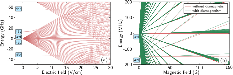
In general, the interaction between an atom and the electromagnetic field can be taken care of by employing the minimal-coupling replacement [124, 125]. Assuming that the fields are static and homogeneous, this general approach gets reduced to adding the electric interaction
| (11) |
and the magnetic interaction
| (12) |
to the Hamiltonian (1), where is the electric dipole operator, and is the magnetic dipole operator. The -factors and characterize the magnetic moment through orbital motion and spin. The constant is the Bohr magneton. The term is the diamagnetic interaction. Most importantly, these formulas allow for electromagnetic fields in arbitrary directions and in particular facilitate arbitrary angles between magnetic and electric fields. The final Hamiltonian is
| (13) |
In order to calculate matrix elements of and , we have to do some preparatory work. In C, we review a powerful formalism to calculate matrix elements of spherical tensor operators. To make use of it, the notation of equations (11) and (12) has to be changed from the cartesian basis to the spherical basis . In the spherical basis the components of, for example, the electric field are given by
| (14) |
Using this expression, the interaction with an electric field reads
| (15) |
with spherical harmonics . Likewise we can express the dot product of and the magnetic field in the spherical basis
| (16) |
where are the spherical momentum operators. The operators are related to the ladder operators and . The diamagnetic interaction in the spherical basis reads
| (17) |
The entire atom-field interaction is now expressed in terms of spherical tensor operators, and we can proceed to calculate the matrix elements via the formalism of B and C. This enables not only the calculation of pair potentials in the presence of external fields but also the computation of Stark/Zeeman maps, see Figure 2.
II.3 Selection rules and symmetries
Knowing how to calculate matrix elements facilitates a rigorous derivation of the selection rules. The results for spherical harmonics and momentum operators are shown in Table 1. Note that the selection rules for spherical harmonics directly apply to the multipole operators. The selection rules greatly reduce the number of matrix elements which must be calculated explicitly for the construction of the pair Hamiltonian, enabling a significant reduction of computation time.
| Spherical harmonics and | Momentum operators |
|---|---|
| multipole operators | |
| not restricted | not restricted |
| and | |
| with | with |
| Symmetry | Conserved | ||||||||
|---|---|---|---|---|---|---|---|---|---|
| operation | quantity | Dipole-dipole | Up to higher orders | ||||||
| Symmetries originating from the point group | |||||||||
| Rotation about -axis | |||||||||
| Reflection through -plane | |||||||||
| Inversion | |||||||||
| Symmetry in case of symmetric interaction potentials | |||||||||
| Permutation | |||||||||
The considered system of two interacting Rydberg atoms has the same symmetries as any diatomic molecule. The point group of the system is / if the system is heteronuclear/homonuclear [126]. The symmetries of the point group are conserved by the Hamiltonian (1) of the two Rydberg atoms in the absence of external fields.
From the symmetry under rotation about the interatomic axis, it follows that the projection of the total angular momentum on the interatomic axis is conserved. Since we have chosen the quantization axis to be parallel to the interatomic axis, the total magnetic quantum number
| (18) |
is conserved.
If the system is homonuclear, a further symmetry is the inversion symmetry (, ). A properly symmetrized basis state is of the form [127, 128, 84]
| (19) |
where for states with gerade symmetry and for states with ungerade symmetry . The Hamiltonian does not couple states of gerade symmetry to states of ungerade symmetry.
Independent of whether the system is homonuclear or heteronuclear, it is symmetric under reflection through a plane containing the interatomic axis [127, 128]. We choose the -plane as mirror plane. The reflection symmetry () can be exploited by changing into the symmetrized basis
| (20) |
with for even states and for odd states under reflection. If the total magnetic quantum number is zero, we can symmetrize with respect to rotation, reflection, and inversion simultaneously. If it is non-zero, this is not possible since then the reflection and the rotation do not commute. In this case, we neglect the reflection symmetry.
In case of pure dipole-dipole interaction, a system of two homonuclear Rydberg atoms is subject to permutation symmetry () in addition to the symmetries of the point group. The interaction potential is symmetric under exchange of the two ionic cores. A properly symmetrized basis state is
| (21) |
where for symmetric states and for antisymmetric states . Comparing equation (19) and (21) shows that
| (22) |
is conserved when both permutation and inversion symmetry are present.
External fields might break the symmetries discussed above. If the operator of the atom-field interaction (11) or (12) does not commute with a symmetry operation, the symmetry is not conserved. For example, external fields that do not point along the interatomic axis can mix states of different total magnetic quantum numbers. Table 2 contains an overview of which symmetry operation commutes with which part of the Hamiltonian (13) of two interacting Rydberg atoms in the presence of external fields.
II.4 Angular dependency

As discussed in section II.1, the formula for the atom-atom interaction (7) is only valid if we are in a coordinate system where the -axis, which we chose as the quantization axis, points in the same direction as the interatomic axis. However, sometimes one would like to use a different coordinate system. For example, when the Rydberg state is excited by a laser pulse, it is convenient to use a coordinate system where the -axis points along the laser beam.
To ease the calculation, let us assume that the interatomic axis lies in the -plane of . Then we can change into by rotating around the -axis, see Figure 3. The rotation angle is defined as the angle between the interatomic axis and the -axis, and is called interaction angle.
Given that our coordinate systems are right-handed and the rotation of the coordinate system is counter-clockwise if the -axis points towards the observer, the magnetic and electric fields transform according to
| (23) |
Any state in the lab frame, i.e. with the quantization axis parallel to the laser beam, should be expressed as a linear superposition of states whose quantization axis points along the -axis of ,
| (24) |
where the coefficients are elements of the Wigner (lowercase) -matrix [129]. If we had not fixed the interatomic axes in the -plane, we would have to use the Wigner (uppercase) -matrix instead. Our notation is consistent with the definitions in [130].
Using the transformations (23) and (24), we can switch to the coordinate system and perform all calculations there.
In the absence of external electromagnetic fields, the eigenvalues of the Hamiltonian and thus the pair potentials do not depend on the interaction angle. However, the overlap of each unperturbed state with a particular eigenstate does depend on the interaction angle. The quantum numbers of the unperturbed state become good quantum numbers if the interatomic distance approaches infinity and the atoms are not perturbed by external fields.

II.5 Matrix diagonalization
In the previous sections, we established the Hamiltonian of two interacting Rydberg atoms and explained how matrix elements of the Hamiltonian can be calculated using B and C. This allows us to compute the matrix representation of the Hamiltonian. We calculate pair potentials of the unperturbed state by numerical diagonalization of the Hamiltonian matrix for a range of interatomic distances. Then, the eigenenergies are plotted versus the distances to make up the pair potentials. By drawing lines between the eigenenergy points for which the overlap between the eigenvectors is maximal, we extract the pair potential curves. The overlap between an eigenvector and the unperturbed state tells the probability to find the unperturbed state on the corresponding pair potential curve.
In order to make the diagonalization of the Hamiltonian computationally feasible, we have to keep the matrix size small. Therefore, it is important to exploit conservation laws. As discussed in section II.3, the Hamiltonian might conserve several quantum numbers and symmetries, leading to a block diagonal structure of the Hamiltonian matrix, see Figure 4 (a).
Each block can be diagonalized independently, which leads to a massive speed-up as the computation of all eigenpairs of a -matrix costs floating-point operations [131, 132]. Furthermore, we diagonalize only those blocks that belong to the unperturbed state we are interested in. In addition, we have to restrict the basis to states having a significant influence on the pair potentials of the unperturbed state.
Hereto, we have several possibilities. First, we can restrict the basis to elements with similar energies as the unperturbed state. Second, it is often useful to constrain the momentum quantum numbers because interaction of high order is required to change the momentum quantum numbers by large values. However, this constraint does not work if states involved in the high order interaction are degenerate as it is the case for Stark map calculations. Third, we can constrain the principal quantum number. If two states do not have similar principal quantum numbers, their radial matrix elements and hence their interaction is negligible, see Figure 4 (b). Higher order interactions, which would only require matrix elements with similar principal quantum numbers, would also be weak as the required order increases with the principal quantum number. How the constraints should be chosen depends on many factors like the considered distances, the required accuracy, the quantum numbers of the unperturbed states, the order of the multipole expansion, external fields, and the atomic species. Thus, giving the right constraints is difficult a priori. In fact, the constraints have to be tested for each calculation. For obtaining a small basis size, we start with strong constraints and loosen them systematically until the pair potentials of the unperturbed state have converged within the distance threshold we are interested in. The convergence is extensively discussed in [84].
For calculating pair potentials in the presence of external electromagnetic fields, the following approach has turned out to be useful: We construct a single-atom basis and calculate the atom-field Hamiltonian for each of the two atoms independently. We enlarge the basis sets until the Stark/Zeeman maps have converged. We combine the eigenstates of the single-atom Hamiltonians into pair states and obtain a pair basis that is suitable for establishing the total Hamiltonian including atom-atom interactions. The combined eigenenergies, that are the Stark/Zeeman energies of the pair states, are located on the diagonal of the Hamiltonian. This procedure has the advantage, that we can now restrict the pair basis to the states relevant for the atom-atom interaction without losing accuracy in the treatment of the electromagnetic fields. Constraining the pair basis stronger than the single-atom basis is appropriate, in particular because the atom-field interaction typically couples over larger energy ranges than the atom-atom interaction. Furthermore, whereas atom-field interactions might change energies drastically, the small amount of admixed states is irrelevant for the atom-atom interaction in many cases of practical relevance. Despite these actions, the inclusion of electromagnetic fields can drastically increase the computational cost. Depending on the type of field, the block structure of the Hamiltonian matrix is destroyed.
III Applications of the Rydberg potential calculation
In this section, we discuss two examples of the Rydberg potential calculation with relevance to recent experiments. Comparison with experimental results enables us to validate our numerical results and demonstrate the applicability of full potential calculations to state-of-the-art experiments. It also allows us to benchmark the influence of the basis size and of the truncation order on the interaction potentials.
III.1 Relevance of higher-order multipole terms and basis size

The relevance of multipole terms in the interaction potential of order higher than dipole-dipole, i.e. in equation (9), has been highlighted in several recent experiments [82, 94, 25, 84]. As an example, we focus here on the observation of Rydberg aggregation dynamics in a vapor cell at room temperature by Urvoy et al. [25]. In this experiment, the high atomic densities and the spectral width of the laser pulses allow to probe Rydberg interaction at short interatomic distances, with one key finding being that the correlated excitation of Rydberg atoms is driven by the dipole-quadrupole () contribution to the interaction.
Specifically, in the experiment, Rydberg excitation in a Cesium vapor cell is driven by two-photon excitation with red detuning relative to the Rydberg state. The pure van-der-Waals interaction potential resulting from dipole-dipole coupling of two atoms in this state is repulsive, see Figure 5 (a), suggesting that the presence of one Rydberg atom does not increase the excitation probability of further Rydberg atoms by the red-detuned driving lasers.
However, including the dipole-quadrupole interaction () results in admixture of the pair state into several close-lying, attractively interacting pair states (such as and ), as shown in Figure 5 (b). As done in [25], we quantify the admixture of, for example, to any Rydberg pair state by . Any such admixture at detuning results in efficient optical excitation of additional Rydberg atoms at specific distances to a first seed excitation. In particular, Urvoy et al. identified the resulting resonance at (where is the Le Roy radius), which is reproduced by our calculations, as the dominant underlying mechanism for the correlated Rydberg aggregation observed in the experiment [25].
Based on this finding, an obvious question is how additional multipole orders further modify the interaction potential. In Figure 5 (c), we show the resulting potential map when the terms, corresponding to quadrupole-quadrupole and dipople-octupole interactions, are included. Significant effects of these contributions can be seen at small interatomic distances , for example in the detuning region between and . For the experiment, the relevant figure is , we show the extracted values for all three potential calculations ( in Figure 5 (d). While the inclusion of the terms also modifies at short distances, the main relevant resonance feature at is not modified by the higher-order terms. Thus, the quantitative differences in the potential landscape due to the next higher-order terms do not affect the conclusions in [25].
In contrast, the features at small distances are relevant for example for formation of bound pair states of Rydberg atoms [79, 82, 83, 80, 81], requiring inclusion of even further orders in the calculation [81, 84]. In general, when increasing , care has to be taken that the pair state basis truncation is appropriately adapted to include enough coupled states. In this example, we have used the constraints and on the differences in quantum numbers of the individual Rydberg states with respect to the state . These cutoff criteria are motivated by the selection rules for the different interaction orders discussed in section II.3 and the scaling of the electric multipole matrix elements, see section II.5. Of particular importance for precise calculations at distances are the symmetry considerations of section II.3, which help to greatly reduce the size of the relevant pair state basis [84].
III.2 Angular dependence of the interaction near a Förster resonance

In the second example, we demonstrate the calculation of anisotropic Rydberg interactions in the presence of electric and magnetic fields, as discussed in sections II.2 and II.4. In this context, we calculate the interaction potentials measured in the experiments of Ravets et al. in [109]. Here, two single atoms were prepared in their ground state in two tightly focussed optical tweezers. Both the distance between the two atoms and the angle between the interatomic axis and the external fields could be precisely tuned. Using a two-photon excitation scheme, both atoms were excited to the state by applying a -pulse. In the pair state basis and at zero electric field, the state is detuned by from the state . Due to the different polarizabilities of the states, both pair states could be tuned into degeneracy by applying a weak electric field of . With this approach, Ravets et al. could map out the angular shape of the electric dipole-dipole interaction between the two atoms [109].
More specifically, the strength of the interaction was measured by letting the two-atom system evolve after the Rydberg excitation and in the presence of the electric field. After a variable hold time, a second optical -pulse coupling to the state was employed to bring the atoms back to their ground state. By measuring the ground-state population after the full sequence, the time-evolution of the Rydberg pair state population could be reconstructed. Performing this experiment for various angles and fixed distance resulted in the beautiful dipole-dipole pattern of the interaction shown by the blue crosses in Figure 6 (d).
For comparison with the experimental results, we calculate the full potentials for different angles including the finite electric and magnetic fields. Here, the optimized matrix construction discussed in section II.5 is particularly relevant to make precise calculations feasible. As an example, we show in Figure 6 (a) and (b) the potentials obtained for (atoms aligned with respect to the external fields) and , respectively. Besides the energy shifts caused by the interaction, we encode here the probability to find an admixture of the initially prepared unperturbed state in the new eigenstate as a density plot. For , Figure 6 (a) show that a two-level approximation is valid for most of the distances between and . Most importantly, at the experimentally relevant distance , the system can be treated as a two-level system.
However, the situation changes for an angle of , where the two-level approximation breaks down. This is caused by mixing of the different fine structure states of the state and of different magnetic levels coupled for non-zero interaction angles.
From the calculated potentials and more specifically the overlap probabilities , it is straight-forward to calculate the coherent evolution of the interacting Rydberg atom pair. Specifically the time-dependent probability of being in the state in the presence of interaction is given by . Examples for two different angles and are shown in Figure 6 (c). For , we obtain an undamped sinusoidal oscillation with a frequency of , which corresponds to the splitting of the most strongly populated pair potentials. In the case of the significant coupling to multiple other pair states leads to dephasing that effectively damps out the Rabi oscillations. These results agree very well with the experimental time-evolution reported in [109].
In Figure 6 (d), we show all frequencies contributing to the time evolution for and varying , obtained from the energy differences of the pair states to which the initial state couples (red points). The size of each point encodes the relative weight of each frequency, which is proportional to . For comparison, the single frequencies at each extracted from the experiment are shown by the blue crosses. One can see that for and for our calculations find a single dominant contribution, which is in excellent agreement with the experimental data. In contrast, for angles outside these regions, the increased number of pair states contributing to the time evolution explains the damped oscillations measured in the experiment.
IV Conclusions and outlook
In this tutorial, we have reviewed the calculation of interaction potentials between pairs of atoms excited to Rydberg states. Precise knowledge of the full potential landscape has become relevant to a wide range of experiments utilizing Rydberg atoms in recent years. Our goal has been to give a comprehensive summary of all the relevant calculation steps of the Rydberg potential for describing current and future experiments. We reviewed the symmetry properties of the interaction Hamiltonian and the selection rules of the different multipole orders. These considerations are crucial for efficient calculation of the interaction potentials. Two further aspects important for experiments are the angular dependence of the interaction and the inclusion of external magnetic and electric fields of arbitrary direction. Particularly, electric fields offer the powerful ability to strongly modify the Rydberg interaction by tuning to Förster resonances of Rydberg pair states. To complete our tutorial, we summarize the calculation of Rydberg wave functions and multipole matrix elements in the appendix.
In parallel to this tutorial, we have released our calculation software which implements all the discussed features as an open source project, https://pairinteraction.github.io/. It is our hope that this code is useful to members of the Rydberg community, either for comparison to their own calculations or as a general tool to explore the rich physics of Rydberg interaction. Our software is built such that further extensions are straight-forward, with one obvious next step being the inclusion of more species available for calculation, such as the alkaline earth metals [133, 134] or Holmium [135, 136]. The goal of our open source approach is to stimulate active participation of other developers. With the rapid progress of both experiments and theory investigating interacting Rydberg systems, it seems likely that more features of the Rydberg potentials will be explored and exploited in the future.
Acknowledgements.
We thank Charles Adams, Przemyslaw Bienias, Rick van Bijnen, Antoine Browaeys, Johannes Deiglmayr, Hannes Gorniaczyk, Christian Gross, Julius de Hond, Jan Kumlin, Thierry Lahaye, Igor Lesanovsky, Weibin Li, Robert Löw, Thomas Niederprüm, Herwig Ott, Asaf Paris-Mandoki, Tilman Pfau, Thibault Peyronel, Pierre Pillet, Thomas Pohl, Jonathan Pritchard, Georg Raithel, James Shaffer, Nikola Šibalíc, Johannes Zeiher for important discussions and for testing our pair interaction software. We are very thankful to Antoine Browaeys and Thierry Lahaye for providing their data on the angular dependence of the Förster resonance. This work is funded by the German Research Foundation through Emmy-Noether-grant HO 4787/1-1, GiRyd project HO 4787/1-3, and SFB/TRR21 and the Ministry of Science, Research and the Arts of Baden-Württemberg through RiSC grant 33-7533.-30-10/37/1 and the European Union H2020 FET Proactive project RySQ (grant N. 640378). O.F. acknowledges support from the Minerva Foundation.Appendix
| Li | Na | K | Rb | Cs | |
|---|---|---|---|---|---|
| S1/2 | [137] (1986) | [138] (1992) | [139] (1981) | [140] (2011) | [141] (2016) |
| P1/2 | [137] (1986) | [142] (1995) | [143] (1983) | [116] (2003) | [141] (2016) |
| P3/2 | [137] (1986) | [142] (1995) | [143] (1983) | [116] (2003) | [141] (2016) |
| D3/2 | [144] (1958) | [142] (1995) | [139] (1981) | [140] (2011) | [145] (1982) |
| D5/2 | [144] (1958) | [142] (1995) | [139] (1981) | [140] (2011) | [141] (2016) |
| F5/2,7/2 | [144] (1958) | [146] (1997) | [147] (1956) | [148] (2006) | [149] (1987) |
| G7/2,9/2 | - | [146] (1997) | - | [150] (2006) | [149] (1987) |
| H9/2,11/2 | - | [146] (1997) | - | - | - |
In the appendix, we briefly review the required steps to assemble the Hamiltonian (1) for the interaction potential calculation. As discussed in section II.1, this requires the Rydberg level energies (3), and the matrix elements of the single-atom electric multipole operators (8). Exact calculations of both the energy spectrum and electron wave functions are possible only for the hydrogen atom. We consider Rydberg atoms with a single electron in a highly excited state (principal quantum number ), which behave very similar to hydrogen, since the Rydberg electron is effectively bound to a core with charge number , consisting of the actual nucleus (with charge ) and inner electrons screening the core charge. This results in expressions for the Rydberg level series which are only slightly modified from the well-known hydrogen result and there exist relatively simple approaches to calculating single-electron wave functions that capture the physics of Rydberg atoms very well. The reduction to a single-electron problem is particularly justified for the alkali atoms, because of the closed-shell structure of the inner electrons. But for sufficiently large this treatment also works well for other atomic species, such as the noble gases [151], the alkaline earth metals [134], and even the lanthanides [136].
Appendix A Rydberg energy levels and wave functions
We consider Rydberg states including spin-orbit coupling, because the fine-structure of Rydberg states with low angular momentum is well resolved in current experiments on interacting Rydberg atoms. The Rydberg levels are specified by the quantum numbers of the single Rydberg electron, namely (principal quantum number), (orbital angular momentum), (total angular momentum), and (magnetic quantum number). We neglect the hyperfine splitting caused by the coupling of the electron angular momentum to the nuclear spin . Although experiments are now resolving hyperfine levels of low- Rydberg states up to very high principal quantum numbers [115] and the hyperfine structure of Rydberg states can be a matter of importance in some quantum information experiments [152], the typical splitting for [116, 117] makes the hyperfine level structure (so far) irrelevant for interactions between Rydberg atoms.
A.1 Quantum defects
The energy of Rydberg levels of other species can be concisely written in analogy to the Rydberg expression for hydrogen as
| (25) |
Here, is an effective, non-integer principal quantum number, which contains the species-dependent deviation from hydrogen, while
| (26) |
is the modified Rydberg constant taking into account the species dependent mass of the atomic core. The effective quantum number is found to depend only weakly on , but is mainly determined by the orbital angular momentum . More specifically, the energies of the Rydberg series can be parameterized by introducing the quantum defects , which in turn are written as a series expansion of the form
| (27) |
The coefficients in this polynomial expression are obtained from fits to experimentally measured transition energies for specific species. The fine-structure splitting is usually included in the quantum defects, which results in them depending on the quantum number . The quantum defects decrease rapidly with increasing orbital angular momentum , since for high- states the influence of the non-hydrogenic core on the single Rydberg electron orbit becomes less relevant. Thus, quantum defects have been experimentally determined for Rydberg states with low orbital angular momentum , with the most precise data being available for the Alkali atoms. Table 3 lists the references for the coefficients of the quantum defects for the Alkalis used for the calculations in this tutorial. These quantum defects are also implemented by default in our software, but can be replaced or extended by new values. The accuracy of the quantum defects used to compute the potential energies of Rydberg states is a key element to the precise determination of Rydberg interaction potentials. Note that the closed-form expression 27 is motivated by, but differs from the analytic result obtained in quantum-defect-theory [153, 120] by the fact that appears in the higher-order terms instead of . This truncation “spoils the theoretical significance” of the quantum defects [151], but is of course necessary when fitting experimental data and provides a simple and elegant expression for the energy of Rydberg levels.
Since Rydberg levels become more hydrogen-like with increasing , we can use the analytic expression for hydrogen fine-structure energies for levels without an experimentally determined quantum defect. In addition, we include a correction term proportional to the core dipole polarizability of the considered species:
| (28) |
The derivation of this formula and a detailed discussion of the core polarizability can be found in [1].
A.2 Rydberg electron wave function
Reducing the Rydberg atom to a single electron orbiting an extended core consisting of the atomic nucleus and the inner electrons, enables us to calculate effective single-electron Rydberg wave functions. Most importantly, the more complex structure of the effective core does not lift the spherical symmetry of the problem, thus the usual separation of variables for the Rydberg electron wave function into radial and angular part holds. The angular part is solved analytically and, when fine-structure is included, given by the spin spherical harmonics
Based on this expression, the angular part of the electric multipole moments can be calculated analytically, including the usual multipole selection rules. This is discussed in detail in C. Non-relativistic quantum defect theory provides analytical solutions for the radial part, known as Coulomb functions [154, 120]. The basic idea is to consider large distances from the nucleus, where the screening of the inner electrons results in an effective core charge . There, the radial Schrödinger equation reduces to the well-known hydrogen case, except that the energy eigenvalues of the bound states are fixed via the experimentally determined quantum defects. As a consequence, the resulting solutions depend on the (non-integer) effective principal quantum number :
| (31) |
Here, is the Gamma function, and is the Whittaker function. The Coulomb functions are obtained by solving the hydrogen Coulomb radial equation where the energies corresponding to non-integer principal quantum numbers have already been inserted. These are approximate wave functions with the correct behavior for large and the right binding energy. For the calculation of transition matrix elements between Rydberg states, these are the important criteria. A relativistic generalization of the quantum-defect theory exists [155], but for the high- Rydberg states of interest here, the modification of the radial wave function due to the fine-structure correction turns out to be negligible.
An alternative approach to obtaining single-electron wave functions is numerically solving the radial Schrödinger equation including a species-dependent model potential [156]. Compared to quantum-defect theory this approach enables calculation of wave functions in the inner region if the model potentials were correctly determined. Typically, the model potential contains three contributions:
| (32) |
Here, is a modified Coulomb potential describing the distance dependent screening of the core charge by the inner electrons, describes the core polarization due to the Rydberg electron, and is the spin-orbit coupling. The different terms are chosen such that the eigenvalues from the numerical solution of the radial Schrödinger equation reproduce the experimentally measured Rydberg energies. If in turn the energies are fixed, the radial Schrödinger equation reduces to a one-dimensional differential equation, and the electron wave functions can be obtained simply by numerical integration (usually from outside to inside). This approach, as well as the analytic Coulomb functions, are implemented in our software. In particular, for the alkali atoms we use expressions for and introduced by Marinescu et al. [157], which yield very good agreement with experimentally observed Rydberg level energies [158]. In the model potential by Marinescu et al., the Coulomb interaction with the smeared out charge distribution of the inner shells is written as:
| (33) |
with coefficients depending on the atomic species and the orbital angular momentum [157]. For the core polarization, only the leading dipole term is considered, which results in:
| (34) |
Here, is again the core dipole polarizability and is the effective core size, obtained by comparing the numerical solutions with the experimentally observed energy levels. In addition to these two terms, we add an effective expression for the spin-orbit interaction [159]
| (35) |
This expression is only valid for large and for smaller distances from the core the full expression derived from the Dirac equation has to be taken into account [156].
The spin-orbit interaction depends on the radial coordinate , thus the numerical radial wave function depends on the total angular momentum . In practice, one usually does not solve the radial Schrödinger equation as eigenvalue problem, but instead inserts the level energies determined from experimental quantum defects (28). Here, care must be taken when combining model potentials (e.g. from [157]) with independently measured quantum defects, since the inserted energies most likely are not eigenenergies of the model potential. Improvements to the model potentials including the fine structure term have recently been discussed by Sanayei et al. [160].
We compare example wave functions obtained via numerical integration with the corresponding Coulomb wave functions in figure 7. The analytic Coulomb wave functions only indirectly include spin-orbit coupling and the modifications of the Coulomb potential from the simple hydrogen case via the quantum defects, while the model potential explicitly includes these effects in the Hamiltonian. For large , and even more so for large , the overlap of the Rydberg electron with the core region is vanishingly small, making the Coulomb functions very accurate solutions.
Appendix B Radial matrix elements
Calculating the radial parts of the electric multipole matrix elements appearing in the interaction Hamiltonian ((7) in section II.1) amounts to solving integrals of the form
| (36) |
where are the radial wave functions discussed in A, obtained either numerically or in the form of Coulomb functions (31), and is the order of the multipole operator from (8) in section II.1. Note, that the radial wave functions obtained by either approach are real, so that the complex conjugation in the matrix element can be omitted. The matrix elements can be straightforwardly calculated by numerical integration [154, 162]. To optimize the numerics it is useful to rescale the radial coordinate and the wave functions according to
| (37) |
This scaling keeps the number of grid points between nodes of the wave function constant [163]. As an alternative to numerical integration, various analytical expressions for electric dipole matrix elements exist [163, 164, 161]. In Figure 8, we compare electric dipole matrix elements obtained from numerical integration either using Coulomb functions or model potential wave functions and evaluation of the analytical expression in [161]. For transitions between low- states the three methods produce remarkable agreement for . For high- transitions there are systematic deviations between the model potential results and the other two approaches, but the relative difference remains smaller than .
It is important to note that the rather simple methods of calculating single-electron wave functions only yield accurate results for . Significantly more advanced methods for calculating energy levels and matrix elements than what we present here have been developed for low- states, see e.g. [165, 166].
Appendix C Angular matrix elements
In addition to the radial part discussed in B, we also need the angular part of the electric multipole matrix elements. In this appendix, we review the general formalism for calculating matrix elements of spherical tensor operators, which can be applied to determine the angular parts appearing when the multipole operators are expressed in the spherical basis. A more comprehensive discussion of this topic can be found for example in [167]. The formalism relies on the Wigner-Eckart theorem [129], which states that matrix elements of spherical tensor operators can be expressed as products of a Wigner 3-j symbol (alternatively a Clebsch-Gordan coefficient) and a reduced matrix element, which is independent of the angular momentum orientation. As we perform calculations in the fine-structure basis, we show the Wigner-Eckart theorem for the total angular momentum . It reads
where is the reduced matrix element for the total angular momentum. In case of the Wigner-Eckart theorem for the orbital angular momentum or spin , the reduced matrix element or would occur instead.
If commutes with the spin , we can relate the different reduced matrix elements via the equation
where the last term is the Wigner 6-j symbol. If commutes with the orbital angular momentum , we have the relation
These equations facilitate the calculation of arbitrary matrix elements, provided that we know the value of the reduced matrix element or , respectively. If the considered spherical tensor operator is a spherical harmonic , it commutes with the spin and the value of the relevant reduced matrix element is
| (44) |
Given that spherical harmonics are proportional to the angular part of the multipole operator , we can evaluate multipole matrix elements as well. In order to calculate matrix elements of the momentum operators , we need the reduced matrix element
| (45) |
References
- [1] T. F. Gallagher, Rydberg Atoms (Cambridge University Press, 1994).
- [2] M. Saffman, T. G. Walker, and K. Mølmer, Rev. Mod. Phys. 82, 2313 (2010).
- [3] D. Jaksch, J. I. Cirac, P. Zoller, S. L. Rolston, R. Côté, and M. D. Lukin, Phys. Rev. Lett. 85, 2208 (2000).
- [4] M. D. Lukin, M. Fleischhauer, R. Cote, L. M. Duan, D. Jaksch, J. I. Cirac, and P. Zoller, Phys. Rev. Lett. 87, 037901 (2001).
- [5] W. R. Anderson, J. R. Veale, and T. F. Gallagher, Phys. Rev. Lett. 80, 249 (1998).
- [6] I. Mourachko, D. Comparat, F. de Tomasi, A. Fioretti, P. Nosbaum, V. M. Akulin, and P. Pillet, Phys. Rev. Lett. 80, 253 (1998).
- [7] K. Singer, M. Reetz-Lamour, T. Amthor, L. G. Marcassa, and M. Weidemüller, Phys. Rev. Lett. 93, 163001 (2004).
- [8] D. Tong, S. M. Farooqi, J. Stanojevic, S. Krishnan, Y. P. Zhang, R. Côté, E. E. Eyler, and P. L. Gould, Phys. Rev. Lett. 93, 063001 (2004).
- [9] T. C. Liebisch, A. Reinhard, P. R. Berman, and G. Raithel, Phys. Rev. Lett. 95, 253002 (2005).
- [10] T. Vogt, M. Viteau, J. Zhao, A. Chotia, D. Comparat, and P. Pillet, Phys. Rev. Lett. 97, 083003 (2006).
- [11] R. Heidemann, U. Raitzsch, V. Bendkowsky, B. Butscher, R. Löw, L. Santos, and T. Pfau, Phys. Rev. Lett. 99, 163601 (2007).
- [12] C. S. E. van Ditzhuijzen, A. F. Koenderink, J. V. Hernández, F. Robicheaux, L. D. Noordam, and H. B. v. L. van den Heuvell, Phys. Rev. Lett. 100, 243201 (2008).
- [13] A. Reinhard, K. C. Younge, T. C. Liebisch, B. Knuffman, P. R. Berman, and G. Raithel, Phys. Rev. Lett. 100, 233201 (2008a).
- [14] R. Heidemann, U. Raitzsch, V. Bendkowsky, B. Butscher, R. Löw, and T. Pfau, Phys. Rev. Lett. 100, 033601 (2008).
- [15] U. Raitzsch, V. Bendkowsky, R. Heidemann, B. Butscher, R. Löw, and T. Pfau, Phys. Rev. Lett. 100, 013002 (2008).
- [16] M. Reetz-Lamour, T. Amthor, J. Deiglmayr, and M. Weidemüller, Phys. Rev. Lett. 100, 253001 (2008).
- [17] I. I. Ryabtsev, D. B. Tretyakov, I. I. Beterov, and V. M. Entin, Phys. Rev. Lett. 104, 073003 (2010).
- [18] A. Schwarzkopf, R. E. Sapiro, and G. Raithel, Phys. Rev. Lett. 107, 103001 (2011).
- [19] Y. O. Dudin, L. Li, F. Bariani, and A. Kuzmich, Nature Phys. 8, 790 (2012).
- [20] M. Ebert, A. Gill, M. Gibbons, X. Zhang, M. Saffman, and T. G. Walker, Phys. Rev. Lett. 112, 043602 (2014).
- [21] T. M. Weber, M. Höning, T. Niederprüm, T. Manthey, O. Thomas, V. Guarrera, M. Fleischhauer, G. Barontini, and H. Ott, Nature Physics 11, 157 (2015).
- [22] J. Zeiher, P. Schauß, S. Hild, T. Macrì, I. Bloch, and C. Gross, Phys. Rev. X 5, 031015 (2015).
- [23] T. Baluktsian, B. Huber, R. Löw, and T. Pfau, Phys. Rev. Lett. 110, 123001 (2013).
- [24] C. Carr, R. Ritter, C. G. Wade, C. S. Adams, and K. J. Weatherill, Phys. Rev. Lett. 111, 113901 (2013).
- [25] A. Urvoy, F. Ripka, I. Lesanovsky, D. Booth, J. P. Shaffer, T. Pfau, and R. Löw, Phys. Rev. Lett. 114, 203002 (2015).
- [26] E. Urban, T. A. Johnson, T. Henage, L. Isenhower, D. D. Yavuz, T. G. Walker, and M. Saffman, Nature Phys. 5, 110 (2009).
- [27] A. Gaëtan, Y. Miroshnychenko, T. Wilk, A. Chotia, M. Viteau, D. Comparat, P. Pillet, A. Browaeys, and P. Grangier, Nature Phys. 5, 115 (2009).
- [28] T. Wilk, A. Gaëtan, C. Evellin, J. Wolters, Y. Miroshnychenko, P. Grangier, and A. Browaeys, Phys. Rev. Lett. 104, 010502 (2010).
- [29] T. Xia, M. Lichtman, K. Maller, A. W. Carr, M. J. Piotrowicz, L. Isenhower, and M. Saffman, Phys. Rev. Lett. 114, 100503 (2015).
- [30] B. J. Lester, N. Luick, A. M. Kaufman, C. M. Reynolds, and C. A. Regal, Phys. Rev. Lett. 115, 073003 (2015).
- [31] H. Kim, W. Lee, H. G. Lee, H. Jo, Y. Song, and J. Ahn, Nature Communications 7, 13317 (2016).
- [32] D. Barredo, S. de Léséleuc, V. Lienhard, T. Lahaye, and A. Browaeys, Science 354, 1021 (2016).
- [33] M. Endres, H. Bernien, A. Keesling, H. Levine, E. R. Anschuetz, A. Krajenbrink, C. Senko, V. Vuletic, M. Greiner, and M. D. Lukin, Science 354, 1024 (2016).
- [34] D. Møller, L. B. Madsen, and K. Mølmer, Phys. Rev. Lett. 100, 170504 (2008).
- [35] M. Müller, I. Lesanovsky, H. Weimer, H. P. Büchler, and P. Zoller, Phys. Rev. Lett. 102, 170502 (2009).
- [36] H. Weimer, M. Müller, I. Lesanovsky, P. Zoller, and H. P. Büchler, Nature Phys. 6, 382 (2010).
- [37] G. Günter, H. Schempp, M. Robert-de Saint-Vincent, V. Gavryusev, S. Helmrich, C. S. Hofmann, S. Whitlock, and M. Weidemüller, Science 342, 954 (2013).
- [38] D. Barredo, S. Ravets, H. Labuhn, L. Béguin, A. Vernier, F. Nogrette, T. Lahaye, and A. Browaeys, Phys. Rev. Lett. 112, 183002 (2014).
- [39] D. Barredo, H. Labuhn, S. Ravets, T. Lahaye, A. Browaeys, and C. S. Adams, Phys. Rev. Lett. 114, 113002 (2015).
- [40] W. Maineult, B. Pelle, R. Faoro, E. Arimondo, P. Pillet, and P. Cheinet, Journal of Physics B: Atomic, Molecular and Optical Physics 49, 214001 (2016).
- [41] P. Schauß, J. Zeiher, T. Fukuhara, S. Hild, M. Cheneau, T. Macrì, T. Pohl, I. Bloch, and C. Gross, Science 347, 1455 (2015).
- [42] H. Labuhn, D. Barredo, S. Ravets, S. de Léséleuc, T. Macrì, T. Lahaye, and A. Browaeys, Nature 534, 667 (2016).
- [43] O. Firstenberg, C. S. Adams, and S. Hofferberth, Journal of Physics B: Atomic, Molecular and Optical Physics 49, 152003 (2016).
- [44] I. Friedler, D. Petrosyan, M. Fleischhauer, and G. Kurizki, Phys. Rev. A 72, 043803 (2005).
- [45] J. D. Pritchard, D. Maxwell, A. Gauguet, K. J. Weatherill, M. P. A. Jones, and C. S. Adams, Phys. Rev. Lett. 105, 193603 (2010).
- [46] A. V. Gorshkov, J. Otterbach, M. Fleischhauer, T. Pohl, and M. D. Lukin, Phys. Rev. Lett. 107, 133602 (2011).
- [47] E. Shahmoon, G. Kurizki, M. Fleischhauer, and D. Petrosyan, Phys. Rev. A 83, 033806 (2011).
- [48] S. Sevinçli, N. Henkel, C. Ates, and T. Pohl, Phys. Rev. Lett. 107, 153001 (2011).
- [49] T. Peyronel, O. Firstenberg, Q. Liang, S. Hofferberth, A. Gorshkov, T. Pohl, M. Lukin, and V. Vuletic, Nature 488, 57 (2012).
- [50] C. S. Hofmann, G. Günter, H. Schempp, M. Robert-de-Saint-Vincent, M. Gärttner, J. Evers, S. Whitlock, and M. Weidemüller, Phys. Rev. Lett. 110, 203601 (2013).
- [51] Y. O. Dudin and A. Kuzmich, Science 336, 887 (2012).
- [52] L. Li, Y. O. Dudin, and A. Kuzmich, Nature 498, 466 (2013).
- [53] S. Baur, D. Tiarks, G. Rempe, and S. Dürr, Phys. Rev. Lett. 112, 073901 (2014).
- [54] H. Gorniaczyk, C. Tresp, J. Schmidt, H. Fedder, and S. Hofferberth, Phys. Rev. Lett. 113, 053601 (2014).
- [55] D. Tiarks, S. Baur, K. Schneider, S. Dürr, and G. Rempe, Phys. Rev. Lett. 113, 053602 (2014).
- [56] H. Gorniaczyk, C. Tresp, P. Bienias, A. Paris-Mandoki, W. Li, I. Mirgorodskiy, H. P. Büchler, I. Lesanovsky, and S. Hofferberth, Nature Communications 7, 12480 (2016).
- [57] C. Tresp, C. Zimmer, I. Mirgorodskiy, H. Gorniaczyk, A. Paris-Mandoki, and S. Hofferberth, Phys. Rev. Lett. 117, 223001 (2016).
- [58] D. Tiarks, S. Schmidt, G. Rempe, and S. Dürr, Science Advances 2, e1600036 (2016).
- [59] O. Firstenberg, T. Peyronel, Q. Liang, A. V. Gorshkov, M. D. Lukin, and V. Vuletic, Nature 502, 71 (2013).
- [60] J. Otterbach, M. Moos, D. Muth, and M. Fleischhauer, Phys. Rev. Lett. 111, 113001 (2013).
- [61] P. Bienias, S. Choi, O. Firstenberg, M. F. Maghrebi, M. Gullans, M. D. Lukin, A. V. Gorshkov, and H. P. Büchler, Phys. Rev. A 90, 053804 (2014).
- [62] B. Olmos, W. Li, S. Hofferberth, and I. Lesanovsky, Phys. Rev. A 84, 041607 (2011).
- [63] G. Günter, M. Robert-de-Saint-Vincent, H. Schempp, C. S. Hofmann, S. Whitlock, and M. Weidemüller, Phys. Rev. Lett. 108, 013002 (2012).
- [64] D. Maxwell, D. J. Szwer, D. Paredes-Barato, H. Busche, J. D. Pritchard, A. Gauguet, K. J. Weatherill, M. P. A. Jones, and C. S. Adams, Phys. Rev. Lett. 110, 103001 (2013).
- [65] W. Li, D. Viscor, S. Hofferberth, and I. Lesanovsky, Phys. Rev. Lett. 112, 243601 (2014).
- [66] Y.-M. Liu, X.-D. Tian, D. Yan, Y. Zhang, C.-L. Cui, and J.-H. Wu, Phys. Rev. A 91, 043802 (2015).
- [67] G. Pupillo, A. Micheli, M. Boninsegni, I. Lesanovsky, and P. Zoller, Phys. Rev. Lett. 104, 223002 (2010).
- [68] N. Henkel, R. Nath, and T. Pohl, Phys. Rev. Lett. 104, 195302 (2010).
- [69] J. Honer, H. Weimer, T. Pfau, and H. P. Büchler, Phys. Rev. Lett. 105, 160404 (2010).
- [70] M. Mattioli, M. Dalmonte, W. Lechner, and G. Pupillo, Phys. Rev. Lett. 111, 165302 (2013).
- [71] J. B. Balewski, A. T. Krupp, A. Gaj, S. Hofferberth, R. Loew, and T. Pfau, New Journal of Physics 16, 063012 (2014).
- [72] C. Gaul, B. J. DeSalvo, J. A. Aman, F. B. Dunning, T. C. Killian, and T. Pohl, Phys. Rev. Lett. 116, 243001 (2016).
- [73] A. W. Glaetzle, M. Dalmonte, R. Nath, I. Rousochatzakis, R. Moessner, and P. Zoller, Phys. Rev. X 4, 041037 (2014).
- [74] A. W. Glaetzle, M. Dalmonte, R. Nath, C. Gross, I. Bloch, and P. Zoller, Phys. Rev. Lett. 114, 173002 (2015).
- [75] R. M. W. van Bijnen and T. Pohl, Phys. Rev. Lett. 114, 243002 (2015).
- [76] Y.-Y. Jau, A. M. Hankin, T. Keating, I. H. Deutsch, and G. W. Biedermann, Nature Physics 12, 71 (2016).
- [77] J. Zeiher, R. van Bijnen, P. Schauß, S. Hild, J.-y. Choi, T. Pohl, I. Bloch, and C. Gross, Nature Physics , 1095 (2016).
- [78] C. Boisseau, I. Simbotin, and R. Côté, Phys. Rev. Lett. 88, 133004 (2002).
- [79] S. M. Farooqi, D. Tong, S. Krishnan, J. Stanojevic, Y. P. Zhang, J. R. Ensher, A. S. Estrin, C. Boisseau, R. Côté, E. E. Eyler, and P. L. Gould, Phys. Rev. Lett. 91, 183002 (2003).
- [80] K. R. Overstreet, A. Schwettmann, J. Tallant, D. Booth, and J. P. Shaffer, Nature Physics 5, 581 (2009).
- [81] H. Saßmannshausen and J. Deiglmayr, Phys. Rev. Lett. 117, 083401 (2016).
- [82] A. Schwettmann, J. Crawford, K. R. Overstreet, and J. P. Shaffer, Phys. Rev. A 74, 020701 (2006).
- [83] J. Stanojevic, R. Côté, D. Tong, E. E. Eyler, and P. L. Gould, Phys. Rev. A 78, 052709 (2008).
- [84] J. Deiglmayr, Physica Scripta 91, 104007 (2016).
- [85] H. Margenau, Rev. Mod. Phys. 11, 1 (1939).
- [86] M. E. Rose, Journal of Mathematics and Physics 37, 215 (1958).
- [87] P. R. Fontana, Phys. Rev. 123, 1865 (1961).
- [88] A. Dalgarno and W. D. Davidson, Advances in Atomic and Molecular Physics 2, 1 (1966).
- [89] M. R. Flannery, D. Vrinceanu, and V. N. Ostrovsky, J. Phys. B: At. Mol. Opt. Phys. 38, S279 (2005).
- [90] K. Singer, J. Stanojevic, M. Weidemüller, and R. Côté, Journal of Physics B: Atomic, Molecular and Optical Physics 38, S295 (2005).
- [91] A. Reinhard, T. C. Liebisch, B. Knuffman, and G. Raithel, Phys. Rev. A 75, 032712 (2007).
- [92] T. G. Walker and M. Saffman, Phys. Rev. A 77, 032723 (2008).
- [93] D. Comparat and P. Pillet, J. Opt. Soc. Am. B 27, A208 (2010).
- [94] J. Deiglmayr, H. Saßmannshausen, P. Pillet, and F. Merkt, Phys. Rev. Lett. 113, 193001 (2014).
- [95] J. Balewski, A. Krupp, A. Gaj, D. Peter, H. Buchler, R. Low, S. Hofferberth, and T. Pfau, Nature 502, 664 (2013).
- [96] X. Zhang, F. B. Dunning, S. Yoshida, and J. Burgdörfer, Phys. Rev. A 92, 051402 (2015).
- [97] C. Tresp, P. Bienias, S. Weber, H. Gorniaczyk, I. Mirgorodskiy, H. P. Büchler, and S. Hofferberth, Phys. Rev. Lett. 115, 083602 (2015).
- [98] A. Derevianko, P. Kómár, T. Topcu, R. M. Kroeze, and M. D. Lukin, Phys. Rev. A 92, 063419 (2015).
- [99] A. Fioretti, D. Comparat, C. Drag, T. F. Gallagher, and P. Pillet, Phys. Rev. Lett. 82, 1839 (1999).
- [100] T. G. Walker and M. Saffman, J. Phys. B: At. Mol. Opt. Phys. 38, 309 (2005).
- [101] K. A. Safinya, J. F. Delpech, F. Gounand, W. Sandner, and T. F. Gallagher, Phys. Rev. Lett. 47, 405 (1981).
- [102] A. Reinhard, K. C. Younge, and G. Raithel, Phys. Rev. A 78, 060702 (2008b).
- [103] J. Nipper, J. B. Balewski, A. T. Krupp, S. Hofferberth, R. Löw, and T. Pfau, Phys. Rev. X 2, 031011 (2012a).
- [104] J. Nipper, J. B. Balewski, A. T. Krupp, B. Butscher, R. Löw, and T. Pfau, Phys. Rev. Lett. 108, 113001 (2012b).
- [105] J. M. Kondo, D. Booth, L. F. Gonçalves, J. P. Shaffer, and L. G. Marcassa, Phys. Rev. A 93, 012703 (2016).
- [106] K. Afrousheh, P. Bohlouli-Zanjani, D. Vagale, A. Mugford, M. Fedorov, and J. D. D. Martin, Phys. Rev. Lett. 93, 233001 (2004).
- [107] P. Bohlouli-Zanjani, J. A. Petrus, and J. D. D. Martin, Phys. Rev. Lett. 98, 203005 (2007).
- [108] D. B. Tretyakov, V. M. Entin, E. A. Yakshina, I. I. Beterov, C. Andreeva, and I. I. Ryabtsev, Phys. Rev. A 90, 041403 (2014).
- [109] S. Ravets, H. Labuhn, D. Barredo, T. Lahaye, and A. Browaeys, Phys. Rev. A 92, 020701 (2015).
- [110] A. Paris-Mandoki, H. Gorniaczyk, C. Tresp, I. Mirgorodskiy, and S. Hofferberth, Journal of Physics B: Atomic, Molecular and Optical Physics 49, 164001 (2016).
- [111] N. Šibalić, J. D. Pritchard, C. S. Adams, and K. J. Weatherill, arXiv:1612.05529 (2016).
- [112] R. J. Le Roy, Canadian Journal of Physics 52, 246 (1974).
- [113] H. Bethe and E. Salpeter, Quantum mechanics of one- and two-electron atoms (Springer, 1957).
- [114] M. Born and R. Oppenheimer, Annalen der Physik 389, 457 (1927).
- [115] H. Saßmannshausen, F. Merkt, and J. Deiglmayr, Phys. Rev. A 87, 032519 (2013).
- [116] W. Li, I. Mourachko, M. W. Noel, and T. F. Gallagher, Phys. Rev. A 67, 052502 (2003).
- [117] A. Tauschinsky, R. Newell, H. B. van Linden van den Heuvell, and R. J. C. Spreeuw, Phys. Rev. A 87, 042522 (2013).
- [118] I. I. Beterov and M. Saffman, Phys. Rev. A 92, 042710 (2015).
- [119] Y. Zeng, P. Xu, X. D. He, Y. Y. Liu, M. Liu, J. Wang, D. J. Papoular, G. V. Shlyapnikov, and M. S. Zhan, arXiv:1702.00349 (2017).
- [120] M. J. Seaton, Reports on Progress in Physics 46, 167 (1983).
- [121] H. B. G. Casimir and D. Polder, Phys. Rev. 73, 360 (1948).
- [122] J. D. Jackson, Classical electrodynamics, 3rd ed. (Wiley, 1998).
- [123] L. Biedenharn, J. Louck, and P. Carruthers, Angular Momentum in Quantum Physics: Theory and Application, Encyclopedia of Mathematics and its Applications (Cambridge University Press, 2009).
- [124] D. A. Steck, Quantum and Atom Optics, available online at http://steck.us/teaching (revision 0.10.6, 25 May 2016).
- [125] P. Milonni, The Quantum Vacuum: An Introduction to Quantum Electrodynamics (Elsevier Science, 2013).
- [126] G. Herzberg, Spectra of diatomic molecules, Molecular spectra and molecular structure (Van Nostrand, 1950).
- [127] J. M. Brown and A. Carrington, Rotational spectroscopy of diatomic molecules (Cambridge University Press, 2003).
- [128] J. Stanojevic, R. Côté, D. Tong, S. Farooqi, E. Eyler, and P. Gould, The European Physical Journal D-Atomic, Molecular, Optical and Plasma Physics 40, 3 (2006).
- [129] E. P. Wigner, Group theory and its application to the quantum mechanics of atomic spectra (Academic Press, 1959).
- [130] D. Varshalovich, A. Moskalev, and V. Khersonskii, Quantum Theory of Angular Momentum (World Scientific Pub., 1988).
- [131] P. Bientinesi, F. D. Igual, D. Kressner, and E. S. Quintana-Ortí, in International Conference on Parallel Processing and Applied Mathematics (Springer, 2009) pp. 387–395.
- [132] J. W. Demmel, O. A. Marques, B. N. Parlett, and C. Vömel, SIAM Journal on Scientific Computing 30, 1508 (2008).
- [133] S. Mauger, J. Millen, and M. P. A. Jones, J. Phys. B: At. Mol. Opt. Phys. 40, F319 (2007).
- [134] C. L. Vaillant, M. P. A. Jones, and R. M. Potvliege, Journal of Physics B: Atomic, Molecular and Optical Physics 45, 135004 (2012).
- [135] M. Saffman and K. Mølmer, Phys. Rev. A 78, 012336 (2008).
- [136] J. Hostetter, J. D. Pritchard, J. E. Lawler, and M. Saffman, Phys. Rev. A 91, 012507 (2015).
- [137] P. Goy, J. Liang, M. Gross, and S. Haroche, Phys. Rev. A 34, 2889 (1986).
- [138] M. Ciocca, C. E. Burkhardt, J. J. Leventhal, and T. Bergeman, Phys. Rev. A 45, 4720 (1992).
- [139] C.-J. Lorenzen, K. Niemax, and L. Pendrill, Optics Communications 39, 370 (1981).
- [140] M. Mack, F. Karlewski, H. Hattermann, S. Höckh, F. Jessen, D. Cano, and J. Fortágh, Phys. Rev. A 83, 052515 (2011).
- [141] J. Deiglmayr, H. Herburger, H. Saßmannshausen, P. Jansen, H. Schmutz, and F. Merkt, Phys. Rev. A 93, 013424 (2016).
- [142] S. F. Dyubko, M. N. Efimenko, V. A. Efremov, and S. V. Podnos, Quantum Electronics 25, 914 (1995).
- [143] C.-J. Lorenzen and K. Niemax, Physica Scripta 27, 300 (1983).
- [144] I. Johansson, Ark. Fysik 15, 169 (1958), as cited in [143].
- [145] P. Goy, J. M. Raimond, G. Vitrant, and S. Haroche, Phys. Rev. A 26, 2733 (1982).
- [146] S. Dyubko, V. Efremov, S. Podnos, X. Sun, and K. B. MacAdam, Journal of Physics B: Atomic, Molecular and Optical Physics 30, 2345 (1997).
- [147] P. Risberg, Ark. Fysik 10, 583 (1956), as cited in [143].
- [148] J. Han, Y. Jamil, D. V. L. Norum, P. J. Tanner, and T. F. Gallagher, Phys. Rev. A 74, 054502 (2006).
- [149] K.-H. Weber and C. J. Sansonetti, Phys. Rev. A 35, 4650 (1987).
- [150] K. Afrousheh, P. Bohlouli-Zanjani, J. A. Petrus, and J. D. D. Martin, Phys. Rev. A 74, 062712 (2006).
- [151] G. W. F. Drake and R. A. Swainson, Phys. Rev. A 44, 5448 (1991).
- [152] K. M. Maller, M. T. Lichtman, T. Xia, Y. Sun, M. J. Piotrowicz, A. W. Carr, L. Isenhower, and M. Saffman, Phys. Rev. A 92, 022336 (2015).
- [153] M. J. Seaton, Monthly Notices of the Royal Astronomical Society 118, 504 (1958).
- [154] D. R. Bates and A. Damgaard, Philosophical Transactions of the Royal Society of London A: Mathematical, Physical and Engineering Sciences 242, 101 (1949).
- [155] W. R. Johnson and K. T. Cheng, Journal of Physics B: Atomic and Molecular Physics 12, 863 (1979).
- [156] C. E. Theodosiou, Phys. Rev. A 30, 2881 (1984).
- [157] M. Marinescu, H. R. Sadeghpour, and A. Dalgarno, Phys. Rev. A 49, 982 (1994).
- [158] M. Pawlak, N. Moiseyev, and H. R. Sadeghpour, Phys. Rev. A 89, 042506 (2014).
- [159] C. H. Greene and M. Aymar, Phys. Rev. A 44, 1773 (1991).
- [160] A. Sanayei, N. Schopohl, J. Grimmel, M. Mack, F. Karlewski, and J. Fortágh, Phys. Rev. A 91, 032509 (2015).
- [161] G. L. Kamta, S. G. N. Engo, M. G. K. Njock, and B. Oumarou, Journal of Physics B: Atomic, Molecular and Optical Physics 31, 963 (1998).
- [162] M. L. Zimmerman, M. G. Littman, M. M. Kash, and D. Kleppner, Phys. Rev. A 20, 2251 (1979).
- [163] S. A. Bhatti, C. L. Cromer, and W. E. Cooke, Phys. Rev. A 24, 161 (1981).
- [164] B. Kaulakys, J. Phys. B: At. Mol. Opt. Phys. 28, 4963 (1995).
- [165] M. S. Safronova and U. I. Safronova, Phys. Rev. A 83, 052508 (2011).
- [166] M. S. Safronova, U. I. Safronova, and C. W. Clark, Phys. Rev. A 94, 012505 (2016).
- [167] I. I. Sobelman, Atomic Spectra and Radiative Transitions (Springer, 1992).