Active Learning and Proofreading
for Delineation of Curvilinear Structures
Abstract
Many state-of-the-art delineation methods rely on supervised machine learning algorithms. As a result, they require manually annotated training data, which is tedious to obtain. Furthermore, even minor classification errors may significantly affect the topology of the final result. In this paper we propose a generic approach to addressing both of these problems by taking into account the influence of a potential misclassification on the resulting delineation. In an Active Learning context, we identify parts of linear structures that should be annotated first in order to train a classifier effectively. In a proofreading context, we similarly find regions of the resulting reconstruction that should be verified in priority to obtain a nearly-perfect result. In both cases, by focusing the attention of the human expert on potential classification mistakes which are the most critical parts of the delineation, we reduce the amount of required supervision. We demonstrate the effectiveness of our approach on microscopy images depicting blood vessels and neurons.
Keywords: Active Learning, Proofreading, Delineation, Light Microscopy, Mixed Integer Programming
1 Introduction
Complex and extensive curvilinear structures include blood vessels, pulmonary bronchi, nerve fibers and neuronal networks among others. Many state-of-the-art approaches to automatically delineating them rely on supervised Machine Learning techniques. For training purposes, they require annotated ground-truth data in large quantities to cover a wide range of potential variations due to imaging artifacts and changes in acquisition protocols. For optimal performance, these variations must be featured in the training data, as they can produce drastic changes in appearance. Furthermore, no matter how well-trained the algorithms are, they will continue to make mistakes, which must be caught by the user and corrected. This is known as proofreading – a slow, tedious and expensive process when large amounts of image data or 3D image stacks are involved, to the point that it is considered as a major bottleneck for applications such as neuron reconstruction [PLZM11].



 |
 |
| (a) | (b) |
In other words, human intervention is required both to create training data before running the delineation algorithm and to correct its output thereafter. Current approaches to making this less tedious focus on providing better visualization and editing tools [DHO14, PLZM11]. While undoubtedly useful, this is not enough. We therefore propose an Active Learning (AL) [Set10] approach to direct the annotator’s attention to the most critical samples. It takes into account the expected change in reconstruction that can result from labeling specific paths. It can be used both for fast annotation purposes and, later, to detect potential mistakes in machine-generated delineations.
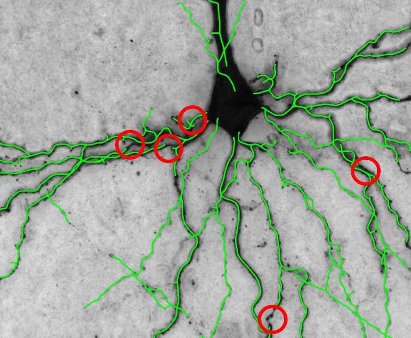
More specifically, consider an algorithm such as those of [SPHHP+15, ZWLS14, TBA+16, NGN+15, PLM11], whose workflow is depicted by Fig. 1. It first builds a graph whose nodes are points likely to lie on the linear structures and whose edges represent paths connecting them. Then it assigns a weight to each edge based on the output of a discriminative classifier. Since the result is critically dependent on the weights, it is important that the classifier is trained well. Finally, the reconstruction algorithm finds a subgraph that maximizes an objective (cost) function dependent on the edge weights, subject to certain constraints. However, even very small mistakes can result in very different delineations, as shown in Fig. 2.
Our main insight is that the decision about which edges to annotate or proofread should be based on their influence on the cost of the network. Earlier methods either ignore the network topology altogether [FRD14] or only take it into consideration locally [MSGF16], whereas we consider it globally. Our contribution is therefore a cost- and topology-based criterion for detecting attention-worthy edges. We demonstrate that this can be used for both AL and proofreading, allowing us to drastically reduce the required amount of human intervention when used in conjunction with the algorithm of [TBA+16]. To make it practical for interactive applications, we also reformulate the latter to speed it up considerably – it runs nearly in real-time and it can handle much larger graphs than [TBA+16].
The remainder of this paper is organized as follows. First, in Section 2, we describe our attention mechanism for selecting important edges in the delineation. In Section 3 we explain how this mechanism can be used for Active Learning and proofreading purposes. Then, in Section 4, we introduce a new, more efficient formulation of the state-of-the-art Mixed Integer Programming delineation algorithm that ensures fast and reliable reconstruction. Finally, in Section 5, we compare the performance of our algorithm against conventional techniques.
2 Attention Mechanism
2.1 Graph-Based Delineation
Delineation algorithms usually start by computing a tubularity measure [LC08, TBG+13, STLF16], which quantifies the likelihood that a tubular structure is present at a given image location. Next, they extract either high-tubularity superpixels likely to be tubular structure fragments [SPHHP+15, ZWLS14] or longer paths connecting points likely to be on the centerline of such structures [GFF08, BSBZ13, NGN+15, TBA+16]. Each superpixel or path is treated as an edge of an over-complete spatial graph (see Fig. 1(a)) and is characterized by an image-based feature vector . Let be the set of all such edges, which is expected to be a superset of the set of edges defining the true curvilinear structure, as shown in Fig. 1(d). If the events of each edge being present in the reconstruction are assumed to be independent (conditional on the image evidence ), then the most likely subset is the one minimizing
| (1) |
where is the weight assigned to edge and is a binary class label denoting whether belongs to the final reconstruction or not. This optimization is subject to certain geometric constraints; for example, a state-of-the-art method presented in [TBA+16] solves a more complex Mixed Integer Program (MIP), which uses linear constraints to force the reconstruction to form a connected network (or a tree). As described in Section 1 of the supplementary material, we were able to reformulate the original optimization scheme and obtain major speedups which make it practical even when delineations must be recomputed often. There, we also show that it yields better results than using a more basic method Minimum Spanning Tree with Pruning [GFF08], while also being able to handle non-tree networks. Let us remark that finding the minimizing is trivial to parallelize.
The probabilities appearing in Eq. 1 can be estimated in many ways. A simple and effective one is to train a discriminative classifier for this purpose [BSBZ13, ZWLS14, TBA+16]. However, the performance critically depends on how well-trained the classifier is. A few misclassified edges can produce drastic topology changes, affecting the whole reconstruction, as shown in Fig. 2. In this paper we address both issues with a single generic criterion.
2.2 Error Detection
The key to both fast proofreading and efficient AL is to quickly find potential mistakes, especially those that are critical for the topology. In this work, we take critical mistakes to mean erroneous edge weights that result in major changes to the cost of the reconstruction. In other words, if changing a specific weight can significantly influence the delineation, we must ensure that the weight is correct. We therefore measure this influence, alter the edge weights accordingly, and recompute the delineation.
2.2.1 Delineation-Change Metric
We denote by the edge subset minimizing the objective (cost) function given a particular set of weights assigned to edges in . Changing the weight of edge to will lead to a new graph with optimal edge subset . We can thus define a delineation-change metric, which evaluates the cost of changing the weight of an edge :
| (2) |
If , the cost has decreased; we can conjecture that the overall reconstruction benefits from this weight change and therefore the weight value may be worth investigating by the annotator as a potential mistake. The converse is true if . In other words, this very simple metric gives us a way to gauge the influence of an edge weight on the overall reconstruction.
2.2.2 Changing the Weights


For our cost change criterion to have practical value, we must alter weights in such a way that is largest for edges which require the opinion of an annotator. In practice, the weights of positive-class edges tend to follow a Gaussian distribution with negative mean and a variance such that few of them are positive values, as shown in Fig. 3(a). Similarly, negative edges follow a Gaussian distribution with positive mean, few of them being negative. As a result, most of the mistaken edges have .
In order for our delineation-change metric to be informative, we must ensure that attention-worthy edges (probable mistakes) have high values of . To achieve this, we must not only flip the sign of the weight (implying assigning it to the opposite class), but also increase the absolute value of likely mistakes. Without this, many of the mistakes with could be omitted due to smaller values of compared to edges with weights of higher absolute value, which are much less likely to be mistakes.
The above requirements can be satisfied with the following transformation:
| (3) |
It is equivalent to swapping the distributions corresponding to positive and negative edges, as shown in Fig 3(b).
We take and to be the 10% and 90% quantiles of the weight distribution (for robustness to outliers). These are near-extreme values of the weights for the positive and negative classes respectively, which we use as attractors for : for small positive we want to be close to , and for negative ones to instead. The weight change is therefore likely to yield a significant for probable mistakes.
Finally, for edges whose weight is negative but which nevertheless do not belong to the graph, we take to be to ensure that it is positive and that more uncertain edges are assigned higher .
3 Active Learning and Proofreading
AL aims to train a model with minimal user input by selecting small subsets of examples that are the most informative. Formally, our algorithm starts with a small set of labeled edges . We then repeat the following steps: At iteration , we use the annotated set of edges to train classifier and select one or more edges to be labeled by the user and added to to form . The edge(s) we select are those that maximize the criterion of Eq. 2.
By contrast, proofreading occurs after the classifier has been trained and a complete delineation has been produced. At this point, the main concern is not to further improve the classifier, but simply to correct potential mistakes. Therefore, the most crucial edges are those that are misclassified and whose presence or absence most affects the topology of the delineation. To find them, we again compute the value for each edge. However, some edges could have a high because they are misclassified, even though they do not influence the topology of the final delineation.
To focus on potential mistakes that do affect the topology strongly, we rely on the DIADEM score [ASL10], which captures the topological differences between trees, such as connectivity changes and missing or spurious branches. It ranges from 0 to 1; the larger the score, the more similar the two trees are. More specifically, let be the optimal tree given the edge weights, and let be the tree we obtain when changing the weight of edge from to , as described in Section 2.2.2. To measure the importance of each edge, we compute the score
| (4) |
and ask the user to check the highest-scoring one. The edge is assigned a weight equal to or from Section 2.2.2 according to the user’s response. We then recompute and repeat the process. Note that this is very different from traditional proofreading approaches, which require the user to visually inspect the whole image. By contrast, our user only has to give an opinion about one edge at a time, which is automatically selected and presented to them.
4 Fast Reconstruction of Curvilinear Structures
To delineate networks of curvilinear structures, we rely on the algorithm of [TBA+16], which involves solving the following problem:
Min-Weight Tree Containing (MinTree)
- Given:
-
A graph , a root vertex , weights on edges . Weights may be negative.
- Find:
-
A tree containing the vertex , minimizing the sum of weights of picked edges .
In our approach, MinTree is used when we expect the ground-truth image to be a tree. If such an assumption is not realistic (loopy networks, such as blood vessels), then we are instead interested in the following problem MinSubgraph:
Min-Weight Connected Subgraph Containing (MinSubgraph)
- Given:
-
A graph , a root vertex , weights on edges . Weights may be negative.
- Find:
-
A connected subgraph which contains the vertex (and is not necessarily a tree), minimizing the sum of weights of picked edges .
Both problems are significantly harder than the Minimum Spanning Tree problem, because does not need to connect the entire graph and also the weights may be negative. In fact, both problems are NP-complete; we demonstrate this later in Proposition 2. In both [TBA+16] and our approach they are solved using a Mixed Integer Programming (MIP) formulation, which is given as input to the Gurobi solver.11 1 [TBA+16] also introduce a more advanced algorithm, which uses a formulation with quadratic weights, i.e., weights on pairs of adjacent edges, rather than a linear weight function; this makes the computational burden even heavier.
However, the previously considered formulation (see the model Arbor-IP in [TBA+16] and also the model M-DG in [BC15]) has variables and as many constraints. This makes solving it costly for small graphs and impossible for larger ones. Our contribution is a new, linear-size MIP model for this problem.
In Section 4.1 we introduce our formulation and argue about its correctness. In Section 4.2 we prove the NP-hardness of the considered problems. The major running time improvements that the new formulation brings about are measured in Section 5.1.
Let us mention in passing that Blum and Calvo [BC15] also propose a “matheuristic” approach to solving MinTree – although with no optimality guarantees.
4.1 Our Formulation
First, we describe how to obtain a MIP for MinTree. We replace each undirected edge with two directed edges, so as to work with a directed graph. Our objective is to find a directed tree whose each edge is directed away from the root (a so-called -arborescence).
We associate a binary variable with each directed edge , denoting the presence of the edge in the solution . The first two linear constraints to consider are:
- •
- •
an edge can be in the solution only if has an incoming edge in the solution (or ) (7).
These conditions almost require the solution to be an -arborescence, but not quite; namely, there can still appear directed cycles (possibly with some adjoined trees). One way to deal with this issue is to enforce that every non-isolated vertex is connected to the root; this can be done using network flows. The constraints in the previous formulation require that, for every with an incoming edge, there should exist a flow of value from to . However, this leads to a large program ( variables).
Our way around this is to instead require the existence of a single flow from the source vertex to some set of sinks. The main constraints are that:
- •
for every vertex , if has an incoming edge (i.e., is not an isolated vertex in the solution, but is spanned by ), then the inflow into is at least more than the outflow (otherwise it is greater or equal to the outflow) (8),
- •
is supported only on the support of (that is, the flow only uses edges which are used by the solution ) (9).
Since has no edges into the root, neither does . Thus is indeed a flow (within the -subgraph) from the source to the sink set being the set of all active vertices.
We write down our MIP formulation below. We use the following notation: for a subset , is the set of (directed) edges outgoing from vertex , and is the set of (directed) edges incoming into vertex . Thus e.g. is the total -flow outgoing from vertex .
| minimize | ||||||||
| subject to | ||||||||
| (5) | ||||||||
| (6) | ||||||||
| (7) | ||||||||
| (8) | ||||||||
| (9) | ||||||||
The following proposition explains the correctness of our formulation.
Proposition 1.
For any , the corresponding vector is feasible for the MIP formulation22 2 More precisely, there exists such that is feasible for the MIP formulation, where is obtained from by directing all edges to point away from . iff is a tree containing the root .
Proof.
() By (5), edges with form a (directed) subgraph where every vertex has indegree at most 1. It is not hard to see that each connected component of such a graph is either a tree or a cycle (possibly with adjoined trees); the cycle case is impossible if the component contains (by (6)). We show that actually there is no connected component except the one containing . Towards a contradiction suppose that is such a component; we will show that the flow conservation constraints (8) must be violated. Denote by the outgoing edges of , and by the incoming edges. We have and thus, by (9), . However, by summing up (8) over we get ; the left side is but the right side is positive, a contradiction.33 3 The observant reader will notice that the constraint (7) is redundant. However, we keep it for clarity of exposition and because it makes solving the program faster in practice.
() It is easy to see that constraints (5–7) are satisfied by . To obtain the flow, we begin with . Then, for each vertex with , we route unit of flow from to inside (that is, we only use edges with ) and add that flow to . (This is possible since is connected.) This way we will satisfy (8). Since the number of such vertices is at most , any edge will hold at most units of flow, thus satisfying (9). ∎
So far we have discussed MinTree. To get a formulation for MinSubgraph, one only needs to omit the constraint (5) and adjust the constraint (9) to become . Then is obtained from by choosing any spanning tree of and orienting tree edges to point away from and non-tree edges arbitrarily. In the proof of Proposition 1 we route units of flow (rather than unit) for each (now any edge holds at most units of flow). These are the only changes.
4.2 Hardness
In this section we argue that our problems are extremely unlikely to be solvable in polynomial time. This makes solving MIP formulations using state-of-the-art solvers one of the most natural and efficient methods available.
Proposition 2.
The problems MinTree and MinSubgraph are NP-complete.
Proof.
Clearly both are in NP. We will show an NP-hardness reduction from the Steiner tree problem in graphs (STP), which is a well-known NP-hard problem. An instance of STP consists of a graph with weights on edges and a set of terminal vertices . The objective is to find a minimum-weight tree in which connects the set . To obtain an instance of MinTree (or MinSubgraph) from STP, we do the following for each : adjoin a new vertex to using a new edge of weight , where is a very large weight (say ). Then set the root to be any of these new vertices.
To see that an optimal solution of the MinTree instance corresponds to an optimal solution of the STP instance, note that the former must necessarily contain all the new edges (as we set their weight to be so low that it makes sense to select them even if it requires us to also select many positive-weight edges). Since the MinTree solution must be connected, it will therefore connect all the terminal vertices; removing the new edges from the MinTree solution gives an optimal STP solution. (The same reduction also works for MinSubgraph, since the weights of all original edges are positive and thus the optimal solution for MinSubgraph is the same as the optimal solution for MinTree.) ∎
5 Results


We tested our approach on 3-D image stacks depicting retinal blood vessels, rat brain axons and dendrites, and drosophila olfactory projection fibers obtained using either 2-photon or brighfield microscopes, shown in Fig. 4.
We rely on the algorithm of [TBA+16] for the initial overcomplete graphs, the corresponding edge features and the final delineations. To classify edges as being likely to be part of an extended linear structure or not on the basis of local image evidence, we use Gradient Boosted Decision Trees [BRLF13].
5.1 Fast Reconstruction
The runtimes of our formulation compared to the one presented in [TBA+16] are shown in Table 1. The optimization was executed on a 2x Intel E5-2680 v2 system (20 cores). Our formulation can be solved under 6 seconds for all real-world graph examples we have tried; the maximum for the formulation of [TBA+16] is over 6 minutes.
| Axons1 | Axons2 | Axons3 | Axons4 | Axons5 | Axons6 | |
|---|---|---|---|---|---|---|
| # edges | 164 | 223 | 224 | 265 | 932 | 2638 |
| MIP [TBA+16] | 0.91 | 1.04 | 1.19 | 1.45 | 78.3 | 393.7 |
| MIP ours | 0.03 | 0.10 | 0.04 | 0.23 | 0.10 | 5.23 |
| speedup | 26.1x | 10.1x | 27.3x | 6.3x | 743.5 | 75.2x |
| BFNeuron1 | BFNeuron2 | OPF1 | OPF2 | BFNeuron3 | BFNeuron4 | |
|---|---|---|---|---|---|---|
| # edges | 120 | 338 | 363 | 380 | 645 | 2826 |
| MIP [TBA+16] | 0.48 | 2.25 | 1.53 | 1.65 | 2.13 | 308.23 |
| MIP ours | 0.02 | 0.12 | 0.05 | 0.08 | 0.26 | 2.30 |
| speedup | 18.2x | 17.7x | 29.4x | 19.9x | 8.1x | 134.0x |
We also compared the runtimes on randomly generated graphs of various sizes – see Table 2. The speed-ups remain similar. In Table 3 we collect runtimes of our method on larger randomly generated graphs. If we assumed (more or less arbitrarily) 2 seconds to be the threshold of what is practical in an interactive setting (given that this optimization needs to be run multiple times), then we can see that the method of [TBA+16] can deal with graphs of size at most 300, whereas our method copes with graphs having around 2000 edges.
| # edges | 99 | 132 | 220 | 330 | 440 | 660 | 924 | 1320 | 1540 |
|---|---|---|---|---|---|---|---|---|---|
| MIP [TBA+16] | 0.16 | 0.30 | 1.13 | 3.39 | 8.35 | 29.35 | 73.16 | 112.59 | 149.01 |
| MIP ours | 0.03 | 0.04 | 0.06 | 0.12 | 0.15 | 0.29 | 0.36 | 0.67 | 0.42 |
| speedup | 6.1x | 7.5x | 17.9x | 29.4x | 53.9x | 102.8x | 201.8x | 167.8x | 348.1x |
| # edges | 1760 | 2420 | 3520 | 4400 | 5720 | 9900 |
|---|---|---|---|---|---|---|
| MIP ours | 1.60 | 2.71 | 6.59 | 9.57 | 15.52 | 81.55 |
One further practical method for speeding up the solver is to initialize it with a nonzero feasible solution. In cases where we needed to explore a large number of reconstructions resulting from altering just one weight at a time (which was the setting of our paper), we initialized the new solution to the current optimal solution. Note that this scenario makes performance considerations especially relevant, as reconstructions need to be made; even though they can be run in parallel, a high running time of a single MIP solution would make the approach impractical.
5.2 Active Learning
For each image, we start with an overcomplete graph. The initial classifier is trained using 10 randomly sampled examples. Then, we query four edges at a time, as discussed in Section 3, which allows us to update the classifier often enough while decreasing the computational cost. We report results averaged over 30 trials in Fig. 5. Our approach outperforms both naive methods such as Uncertainty Sampling (US) and more sophisticated recent ones such as DPPS [MSGF16] and EMOC [FRD14]. DPPS is designed specifically for delineation and also relies on uncertainty sampling, but only takes local topology into account when evaluating this uncertainty. EMOC is a more generic method that aims at selecting samples that have the greatest potential to change the output.
In Fig. 6 we can see that using MIP formulations indeed helps improve the AL results, compared to a more basic method Minimum Spanning Tree with Pruning [GFF08] (MSTP), as it produces more accurate reconstructions and thus we can more reliably detect mistakes. This is visible especially in case of Blood Vessels, which in reality can form loops. Those can be reconstructed using MinSubgraph MIP, but not with MSTP.
5.3 Proofreading

For each test image, we compute an overcomplete graph and classify its edges using a classifier trained on 20000 samples. We then find four edges with the highest values of the score of Eq. 4 and present them to the user for verification. Their feedback is then used to update the delineation.
The red curves of Fig. 7(a-c) depict the increase in DIADEM score. Rapid improvement can be seen after as few as 15 corrections. Fig. 8 shows how the reconstruction evolves in a specific case. For analysis purposes, we also reran the experiment using the criterion of Eq. 2 (cost-only) instead of the more sophisticated one of Eq. 4 (cost and topology) to choose the paths to be examined. The green curves in Fig. 7(a-c) depict the results. They are not as good, particularly in the case of Fig. 7(c), because the highest-scoring mistakes are often the ones that tend to be in the MIP reconstruction both before and after correcting mistakes. It is therefore only by combining both cost and topology that we increase the chances that a potential correction of the selected edge will improve the reconstruction. By contrast, paths chosen by RS and US are not necessarily erroneous or in the immediate neighborhood of the tree. As a result, investigating them often does not give any improvements.
5.4 Complete Pipeline
In a working system, we would integrate AL and proofreading into a single pipeline. To gauge its potential efficiency, we selected 50 edges to train our classifier using the AL strategy of Section 3. We then computed a delineation in a test image and proofread it by selecting 35 edges. For comparison purposes, we used either our approach as described in Section 3, RS, or US to pick the edges for training and then for verification. In Fig. 7(d) we plot the performance (in terms of the DIADEM score of the final delineation and of the ground truth) as a function of the total number of edges the user needed to label manually.
6 Conclusions
We have presented an attention scheme that significantly reduces the annotation effort involved both in creating training data for supervised Machine Learning and in proofreading results for delineation tasks. It does so by detecting possibly misclassified samples and considering their influence on the topology of the reconstruction. We showed that our method outperforms baselines on a variety of microscopy image stacks and can be used in interactive applications thanks to its efficient formulation.
References
- [ASL10] G. Ascoli, K. Svoboda, and Y. Liu. Digital Reconstruction of Axonal and Dendritic Morphology DIADEM Challenge, 2010. URL: http://diademchallenge.org/.
- [BC15] C. Blum and B. Calvo. A matheuristic for the minimum weight rooted arborescence problem. Journal of Heuristics, 21(4):479–499, 2015.
- [BRLF13] C. Becker, R. Rigamonti, V. Lepetit, and P. Fua. Supervised Feature Learning for Curvilinear Structure Segmentation. In MICCAI, September 2013.
- [BSBZ13] D. Breitenreicher, M. Sofka, S. Britzen, and S.K. Zhou. Hierarchical Discriminative Framework for Detecting Tubular Structures in 3D Images. In International Conference on Information Processing in Medical Imaging, 2013.
- [DHO14] V. Dercksen, H. Hege, and M. Oberlaender. The Filament Editor: An Interactive Software Environment for Visualization, Proof-Editing and Analysis of 3D Neuron Morphology. Neuroinformatics, 12:325–339, 2014.
- [FRD14] A. Freytag, E. Rodner, and J. Denzler. Selecting Influential Examples: Active Learning with Expected Model Output Changes. 2014.
- [GFF08] G. Gonzalez, F. Fleuret, and P. Fua. Automated Delineation of Dendritic Networks in Noisy Image Stacks. In ECCV, pages 214–227, October 2008.
- [LC08] M.W. Law and A.C. Chung. Three Dimensional Curvilinear Structure Detection Using Optimally Oriented Flux. In ECCV, 2008.
- [MSGF16] A. Mosinska, R. Sznitman, P. Glowacki, and P. Fua. Active Learning for Delineation of Curvilinear Structures. In CVPR, 2016.
- [NGN+15] P. F. Neher, M. Götz, T. Norajitra, C. Weber, and K. H. Maier-Hein. A Machine Learning Based Approach to Fiber Tractography Using Classifier Voting. In Medical Image Computing and Computer-Assisted Intervention - MICCAI, pages 45–52, 2015.
- [PLM11] H. Peng, F. Long, and G. Myers. Automatic 3D Neuron Tracing Using All-Path Pruning. 27(13):239–247, 2011.
- [PLZM11] H. Peng, F. Long, T. Zhao, and E.W. Myers. Proof-Editing is the Bottleneck of 3D Neuron Reconstruction: the Problem and Solutions. Neur. Inf., 9(2):103–105, 2011.
- [Set10] B. Settles. Active Learning Literature Survey. Technical report, University of Wisconsin–Madison, 2010.
- [SPHHP+15] A. Santamaría-Pang, P. Hernandez-Herrera, M. Papadakis, P. Saggau, and I.A. Kakadiaris. Automatic Morphological Reconstruction of Neurons from Multiphoton and Confocal Microscopy Images Using 3D Tubular Models. Neur. Inf., pages 1–24, 2015.
- [STLF16] A. Sironi, E. Turetken, V. Lepetit, and P. Fua. Multiscale Centerline Detection. PAMI, 2016.
- [TBA+16] E. Turetken, F. Benmansour, B. Andres, P. Glowacki, H. Pfister, and P. Fua. Reconstructing Curvilinear Networks Using Path Classifiers and Integer Programming. PAMI, 2016.
- [TBG+13] E. Turetken, C. Becker, P. Glowacki, F. Benmansour, and P. Fua. Detecting Irregular Curvilinear Structures in Gray Scale and Color Imagery Using Multi-Directional Oriented Flux. In ICCV, December 2013.
- [ZWLS14] J. A. Montoya Zegarra, J. D. Wegner, L. Ladicky, and K. Schindler. Mind the Gap: Modeling Local and Global Context in (Road) Networks. In Pattern Recognition - 36th German Conference, GCPR 2014, Münster, 2014.