Looking at the deconfinement transition using Wilson flow
Abstract:
Wilson flow is an effective tool for constructing renormalized composite operators. We explore use of the Wilson flow to construct renormalized order parameters for the deconfinement transition in SU(3) gauge theory. We discuss renormalization of the Polyakov loop, and of gluon condensates.
24-30 July 2016
University of Southampton, UK
1 Introduction
Wilson flow, the evolution of the gauge links along the gradient of the gauge action, is a powerful new technique in the study of non-Abelian gauge theories on a lattice [1, 2]. Some of its most common uses have been in scale setting [1, 3] and in renormalization of composite operators, e.g., Refs. [4, 5]. The renormalization of the composite operators can be particularly useful in the context of finite temperature studies of QCD. An early example has been the calculation of pure gauge theory thermodynamics with energy-momentum tensor renormalized using Wilson flow [6]. Here we report on the use of flow to construct an order parameter for the pure gauge theory transition, and to study the behavior of gluon condensates across the transition. More details of our study can be found in Ref. [7].
After Wilson flow to time , the link operators are smeared to a size . Lüscher has suggested defining the scale through a construction involving the gluon condensate. A dimensionful quantity is defined as the flow time such that , where is a suitable number,
| (1) |
is the (discretized) field strength tensor and is the space-time volume. In perturbation theory [4]
| (2) |
In order that effects of the ultraviolet scale is suppressed, should be such that . For scale setting, Lüscher has suggested =0.3; and the corresponding is commonly referred to as . At finite temperature, sets the energy scale of interest; since flow strongly suppresses energy scales , ideally for thermal physics one would like to have
| (3) |
In typical finite temperature lattice studies at present, ; so the strong inequalities in Eq. (3) can at most mean “smaller by a factor 4”. If we want to keep c fixed while the temperature is changed, Eq. (3) can be satisfied only if for all and . In [6], was fixed as one changes . An exploration of these strategies will be reported as part of the study.
We study flow on finite temperature lattices in the temperature range between 0.9 and 3.1 employing four sets of lattices, corresponding to 6, 8, 10 and 12. In each set, temperature is changed by changing ; is set from the peak of the Polyakov loop susceptibility and the relative temperature in the other lattices is set using Wilson flow. The lattices are new; details of the other sets can be found in [7]. First, we discuss the Polyakov loop, which is the order parameter for the deconfinement transition, but is highly singular as one takes the continuum limit. We discuss in the next section the use of flow to construct a continuum order parameter, referred to here as the “flowed Polyakov loop”. Further, we proceed to renormalize the Polyakov loop using this construct. Renormalization of Polyakov loop using Wilson flow has been considered earlier in Ref. [petreczky], while a later paper [10] has discussed various properties of the flowed Polyakov loop and renormalization of Polyakov loop. While we do not have place here to discuss those works, our approach to renormalized Polyakov is different from what has been followed there. In the last section, we discuss the flow-time behavior of various parts of the gluon condensate. It is known that as one crosses the deconfinement temperature the gluon condensate starts to melt. We find that the electric and magnetic components of the condensate have very different flow behaviors, and use them to explore the temperature dependence of the different condensates.
2 Polyakov loop
The deconfinement transition is associated with the breaking of the center symmetry for SU(3) gauge theory. The Polyakov loop,
| (4) |
transforms nontrivially under the symmetry and acts as an order parameter for the transition. Following standard arguments, in finite volume system one monitors the transition by looking at
| (5) |
The bare Polyakov loop, as defined in Eq. (5), depends strongly on
the lattice spacing [11],
| (6) |
approaching as . On the other hand, Wilson flow can be used to define an order parameter that is only mildly dependent on the lattice spacing , and has a finite continuum limit: if we flow to a physical scale , and define a Polyakov loop, through Eq. (4) with the links replaced by flowed links, then . Since the Wilson flow preserves center symmetry, the flowed Polyakov loop can be treated as an order parameter for the deconfinement transition.
In Fig.1, we show the flowed Polyakov loop for four different lattice spacings at two different temperatures. The strong dependence at , indicated by Eq. (6), is removed at finite flow times; the remaining finite corrections are seen to be suppressed when the flow time increases to , i.e, on the respective lattices. This is less restrictive than Eq. (3), and allows one to have a window where finite temperature studies with Wilson flow can be performed on present day lattices.


In Fig. 2 the flowed Polyakov loop is shown at a flow time , at three different lattice spacings. This flow time is large enough that the finite effects are negligible. From now on, we will restrict ourselves to flow times such that finite effects are negligible, and suppress the argument , referring simply to .
This -independent flowed Polyakov loop is sufficient to measure the
continuum deconfinement transition in pure gauge theory. In the right
panel of Fig. 2 we show the susceptibility density
| (7) |
At a first order transition, , is expected to show a volume-independent peak at , just like the susceptibility density for the non-flowed loop. Unlike the latter, however, the flowed susceptibility peak height does not change with , as illustrated in the figure.


We next turn to the extraction of the renormalized Polyakov loop , Eq. (6), from . Since with flow, acts as an inverse momentum cutoff, analogous to Eq. (6) one can write
| (8) |
where, to leading order, [7]
| (9) |
Following standard arguments [11] we expect that is a function of temperature up to corrections, and has a finite limit as .
In order to calculate using Eq. (9), we need to evaluate . In this report we will evaluate by inverting Eq. (2). See Ref. [7] for results with a direct evaluation of from , and comparison with from Eq. (2). In the left panel of Fig. 3, we show calculations of using Eq. (9) at different temperatures, for lattices with and , respectively. While at higher temperatures, the remnant flow time dependence is mild, we see that as one comes closer to it becomes much stronger and an extrapolation to becomes difficult. Also while the finer lattice shows clear improvement at higher temperatures, it still is not good enough to extract close to .


In order to calculate at lower temperatures, we therefore follow a different strategy. Note that the temperature dependence of the renormalization factor is simple, Eq. (8), and therefore, the renormalization factor at a lower temperature can be simply obtained from the renormalization factor at a higher temperature up to remnant linear corrections, which we expect to be small if we remain within a window . In order to extract , we take, as a baseline value, = 1.0169(1) [12]. This determines , which can then be used to calculate to all temperatures upto 2 Ṫhis process is then iterated to calculate at lower temperatures. This strategy is similar in spirit to that followed in Ref. [12]; however, the use of flow makes the calculation simpler, as we do not need to match lattices at different lattice spacings to same temperature. The renormalized Polyakov loop extracted this way is shown in Figure 3.
3 Gluon condensates
The nonperturbative nature of the QCD vacuum is characterized by various condensates. The dimension four, scalar condensate can give rise to two operators at finite temperature,
| (10) |
connected by O(4) transformations.
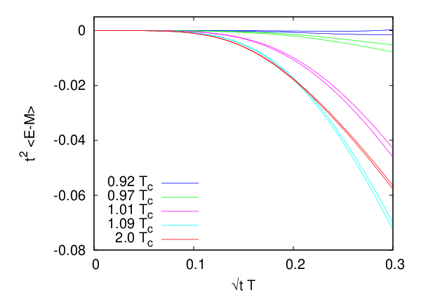
The flow behaviors of and turn out to be quite interesting. In Fig. 4 we show the dimensionless flowed quantities and immediately below and above , together with the corresponding operator at T=0. The figure indicates that O(4) symmetry breaking sets in rather abruptly in a narrow temperature interval near .


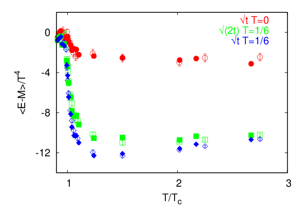
In the left panel of Fig. 5 we show the difference . At large flow times this quantity is very sensitive to the deconfinement transition, remaining very small upto and then showing a jump. In the right panel of the figure we show , for and two different nonzero flow times. The flow behavior of and lead to a sharp jump in this object, which can be used to monitor the traaansition.
The flowed condensates can be used to calculate the conventionally normalized gluon condensates. For this, we first do a vacuum subtraction, i.e., calculate and similarly for . Then the vacuum subtracted finite temperature gluon condensates can be written as [5]
| (11) |
In the left panel of Fig. 6 we show, for illustration, at different flow times. In the coarser lattices, the result is rather disappointing: there is hardly any hint of a plateau or a linear behavior from which one can extract the limit. On the other hand, with the two finest lattices, a plateau starts to form. Further, in the two coarser lattices, the condensate is in agreement with the finer lattices up to this plateau region, but then the lattice spacing effects set in as becomes before formation of a proper plateau. Taking the value in this region to be an approximation to the limit, we show in the right panel of the figure the value of the vacuum subtracted condensates. The result is quite interesting: just above both the condensates show large values. At higher temperatures, while the electric and magnetic condensates themselves do not become insignificant, they have opposite signs, which lead to a small .


The computations reported here were carried out in the gaggle and pride clusters of the department of theoretical physics, TIFR. We thank Ajay Salve and Kapil Ghadiali for technical support.
References
- [1] M. Lüscher, J. High Energy Phys. 1 (0) 08 (2010) 071.
- [2] R. Narayanan and H. Neuberger, J. High Energy Phys. 0 (6) 03 (2006) 064.
- [3] See, e.g., R. Sommer, PoS LATTICE 2013 (2014) 015 (arXiv:1401.3270), and references therein.
- [4] M. Luscher, J. High Energy Phys. 1 (3) 04 (2013) 123.
- [5] H. Suzuki, Prog. Theor. Exp. Phys. (2013) 083B03; Prog. Theor. Exp. Phys. (2015) 103B03.
- [6] M. Asakawa, T. Hatsuda, E. Itou, M. Kitazawa and H. Suzuki, Phys. Rev. D (9) 0 (2014) 011501; Phys. Rev. D (9) 2 (2015) 059902.
- [7] S. Datta, S. Gupta and A. Lytle, arXiv:1512.04892, to be published in Phys. Rev. D (.) petreczky P. Petreczky and H.-P. Schadler, Phys. Rev. D (9) 2 (2015) 094517.
- [10] A. Bazavov, et al., Phys. Rev. D (9) 3 (2016) 114502.
- [11] A.M. Polyakov, Nucl. Phys. B164 (1980) 171.
- [12] S. Gupta, K. Hübner and O. Kaczmarek, Phys. Rev. D (7) 7 (2008) 034503.