Set Similarity Search Beyond MinHashNote: The research leading to these results has received funding from the European Research Council under the European Union’s 7th Framework Programme (FP7/2007-2013) / ERC grant agreement no. 614331.

High-dimensional approximate similarity search methods can be characterized in terms of their $\rho$-value which is the exponent for which queries can be answered in time $O({dn^{\rho}})$, where $n$ is the size of the set $P$ and $d$ denotes the dimensionality of the space. Here we focus on the “balanced” case where we aim for space $O({n^{1+\rho}+dn})$, but note that there now exist techniques for obtaining other trade-offs between query time and space overhead (Andoni et al., 2017; Christiani, 2017).

Locality-Sensitive Hashing Methods. We begin by describing results for Hamming space, which is a special case of similarity search on the unit sphere (many of the results cited apply to the more general case). In Hamming space the focus has traditionally been on the $\rho$-value that can be obtained for solutions to the $(r,cr)$-approximate near neighbor problem: Preprocess a set of points $P\subseteq\{0,1\}^{d}$ such that, given a query point $\mathbf{q}$, if there exists $\mathbf{x}\in P$ with $\lVert\mathbf{x}-\mathbf{q}\rVert_{1}\leq r$, then return $\mathbf{x}^{\prime}\in P$ with $\lVert\mathbf{x}^{\prime}-\mathbf{q}\rVert_{1}<cr$. In the literature this problem is often presented as the $c$-approximate near neighbor problem where bounds for the $\rho$-value are stated in terms of $c$ and, in the case of upper bounds, hold for every choice of $r$, while lower bounds may only hold for specific choices of $r$.

O’Donnell et al. (O’Donnell et al., 2014) have shown that the value $\rho=1/c$ for $c$-approximate near neighbor search in Hamming space, obtained in the seminal work of Indyk and Motwani (Indyk and Motwani, 1998), is the best possible in terms of $c$ for schemes based on Locality-Sensitive Hashing (LSH). However, the lower bound only applies when the distances of interest, $r$ and $cr$, are relatively small compared to $d$, and better upper bounds are known for large distances. Notably, other LSH schemes for angular distance on the unit sphere such as cross-polytope LSH (Andoni et al., 2015) give lower $\rho$-values for large distances. Extensions of the lower bound of (O’Donnell et al., 2014) to cover more of the parameter space were recently given in (Andoni et al., 2017; Christiani, 2017). Until recently the best $\rho$-value known in terms of $c$ was $1/c$, but in a sequence of papers Andoni et al. (Andoni et al., 2014; Andoni and Razenshteyn, 2015) have shown how to use data-dependent LSH techniques to achieve $\rho=1/(2c-1)+o_{n}(1)$, bypassing the lower bound framework of (O’Donnell et al., 2014) which assumes the LSH to be independent of data.

Set Similarity Search. There exists a large number of different measures of set similarity with various applications for which it would be desirable to have efficient approximate similarity search algorithms (Choi et al., 2010). Given a measure of similarity $S$ assume that we have access to a family $\mathcal{H}$ of locality-sensitive hash functions (defined in Section 2) such that for $h\sim\mathcal{H}$ it holds for every pair of sets $\mathbf{x},\mathbf{y}$ that $\Pr[h(\mathbf{x})=h(\mathbf{y})]=S(\mathbf{x},\mathbf{y})$. Then we can use the the LSH framework to construct a solution for the $(s_{1},s_{2})$-approximate similarity search problem under $S$ with exponent $\rho=\log(1/s_{1})/\log(1/s_{2})$. With respect to the existence of such families Charikar (Charikar, 2002) showed that if the similarity measure $S$ admits an LSH with the above properties, then $1-S$ must be a metric. Recently, Chierichetti and Kumar (Chierichetti and Kumar, 2015) showed that, given a similarity $S$ that admits an LSH with the above properties, the transformed similarity $f(S)$ will continue to admit an LSH if $f(\cdot)$ is a probability generating function. The existence of an LSH that admits a similarity measure $S$ will therefore give rise to the existence of solutions to the approximate similarity search problem for the much larger class of similarities $f(S)$. However, this still leaves open the problem of finding efficient explicit constructions, and as it turns out, the LSH property $\Pr[h(\mathbf{x})=h(\mathbf{y})]=S(\mathbf{x},\mathbf{y})$, while intuitively appealing and useful for similarity estimation, does not necessarily imply that the LSH is optimal for solving the approximate search problem for the measure $S$. The problem of finding tight upper and lower bounds on the $\rho$-value that can be obtained through the LSH framework for data-independent $(s_{1},s_{2})$-approximate similarity search across the entire parameter space $(s_{1},s_{2})$ remains open for two of the most common measures of set similarity: Jaccard similarity $J(\mathbf{x},\mathbf{y})=|\mathbf{x}\cap\mathbf{y}|/|\mathbf{x}\cup\mathbf{y}|$ and cosine similarity $C(\mathbf{x},\mathbf{y})=|\mathbf{x}\cap\mathbf{y}|/\sqrt{|\mathbf{x}||\mathbf{y}|}$.

A random function from the MinHash family $\mathcal{H}_{\text{minhash}}$ hashes a set $\mathbf{x}\subset\{1,\dots,d\}$ to the first element of $\mathbf{x}$ in a random permutation of the set $\{1,\dots,d\}$. For $h\sim\mathcal{H}_{\text{minhash}}$ we have that $\Pr[h(\mathbf{x})=h(\mathbf{y})]=J(\mathbf{x},\mathbf{y})$, yielding an LSH solution to the approximate Jaccard similarity search problem. For cosine similarity the SimHash family $\mathcal{H}_{\text{simhash}}$, introduced by Charikar (Charikar, 2002), works by sampling a random hyperplane in ^d that passes through the origin and hashing $\mathbf{x}$ according to what side of the hyperplane it lies on. For $h\sim\mathcal{H}_{\text{simhash}}$ we have that $\Pr[h(\mathbf{x})=h(\mathbf{y})]=1-\arccos(C(\mathbf{x},\mathbf{y}))/\pi$, which can be used to derive a solution for cosine similarity, although not the clean solution that we could have hoped for in the style of MinHash for Jaccard similarity. There exists a number of different data-independent LSH approaches (Terasawa and Tanaka, 2007; Andoni et al., 2014; Andoni et al., 2015) that improve upon the $\rho$-value of SimHash. Perhaps surprisingly, it turns out that these approaches yield lower $\rho$-values for the $(j_{1},j_{2})$-approximate Jaccard similarity search problem compared to MinHash for certain combinations of $(j_{1},j_{2})$. Unfortunately, while asymptotically superior these techniques suffer from a non-trivial $o_{n}(1)$-term in the exponent that only decreases very slowly with $n$. In comparison, both MinHash and SimHash are simple to describe and have closed expressions for their $\rho$-values. Furthermore, MinHash and SimHash both have the advantage of being efficient in the sense that a hash function can be represented using space $O(d)$ and the time to compute $h(\mathbf{x})$ is $O(|\mathbf{x}|)$.

In Table 1 we show how the upper bounds for similarity search under different measures of set similarity relate to each other in the case where all sets are $t$-sparse. In addition to Hamming distance and Jaccard similarity, we consider Braun-Blanquet similarity (Braun-Blanquet, 1932) defined as

which for $t$-sparse vectors is identical to cosine similarity. When the query and the sets in $P$ can have different sizes the picture becomes muddled, and the question of which of the known algorithms is best for each measure $S$ is complicated. In Section 5 we treat the problem of different set sizes and provide a brief discussion for Jaccard similarity, specifically in relation to our upper bound for Braun-Blanquet similarity.

Similarity search under set similarity and the batched version often referred to as set similarity join (Arasu et al., 2006; Bayardo et al., 2007) have also been studied extensively in the information retrieval and database literature, but mostly without providing theoretical guarantees on performance. Recently the notion of containment search, where the similarity measure is the (unnormalized) intersection size, was studied in the LSH framework (Shrivastava and Li, 2015). This is a special case of maximum inner product search (Shrivastava and Li, 2015; Ahle et al., 2016). However, these techniques do not give improvements in our setting.

Similarity Estimation. Finally, we mention that another application of MinHash (Broder, 1997; Broder et al., 1997) is the (easier) problem of similarity estimation, where the task is to condense each vector $\mathbf{x}$ into a short signature $s(\mathbf{x})$ in such a way that the similarity $J(\mathbf{x},\mathbf{y})$ can be estimated from $s(\mathbf{x})$ and $s(\mathbf{y})$. A related similarity estimation technique was independently discovered by Cohen (Cohen, 1997). Thorup (Thorup, 2013) has shown how to perform similarity estimation using just a small amount of randomness in the definition of the function $s(\cdot)$. In another direction, Mitzenmacher et al. (Mitzenmacher et al., 2014) showed that it is possible to improve the performance of MinHash for similarity estimation when the Jaccard similarity is close to 1, but for smaller similarities it is known that succinct encodings of MinHash such as the one in (Li and König, 2011) comes within a constant factor of the optimal space for storing $s(\mathbf{x})$ (Pagh et al., 2014). Curiously, our improvement to MinHash in the context of similarity search comes when the similarity is neither too large nor too small. Our techniques do not seem to yield any improvement for the similarity estimation problem.

We show the following upper bound for approximate similarity search under Braun-Blanquet similarity:

In the case where the sets are $t$-sparse our Theorem 1.1 gives the first strict improvement on the $\rho$-value for approximate Jaccard similarity search compared to the data-independent LSH approaches of MinHash and Angular LSH. Figure 2 shows an example of the improvement for a slice of the parameter space. The improvement is based on a new locality-sensitive mapping that considers a specific random collection of length-$k$ paths on the vertex set $\{1,\dots,d\}$, and associates each vector $\mathbf{x}$ with the paths in the collection that only visits vertices in $\{i\;|\;\mathbf{x}_{i}=1\}$. Our data structure exploits that similar vectors will be associated with a common path with constant probability, while vectors with low similarity have a negligible probability of sharing a path. However, the collection of paths has size superlinear in $n$, so an efficient method is required for locating the paths associated with a particular vector. Our choice of the collection of paths balances two opposing constraints: It is random enough to match the filtering performance of a truly random collection of sets, and at the same time it is structured enough to allow efficient search for sets matching a given vector. The search procedure is comparable in simplicity to the classical techniques of bit sampling, MinHash, SimHash, and $p$-stable LSH, and we believe it might be practical. This is in contrast to most theoretical advances in similarity search in the past ten years that suffer from $o(1)$ terms in the exponent of complexity bounds.

Intuition. Recall that we will think of a vector $\mathbf{x}\in\{0,1\}^{d}$ also as a set, $\{i\;|\;\mathbf{x}_{i}=1\}$. MinHash can be thought of as a way of sampling an element $i_{\mathbf{x}}$ from $\mathbf{x}$, namely, we let $i_{\mathbf{x}}=\argmin_{i\in\mathbf{x}}h(i)$ where $h$ is a random hash function. For sets $\mathbf{x}$ and $\mathbf{y}$ the probability that $i_{\mathbf{x}}=i_{\mathbf{y}}$ equals their Jaccard similarity $J(\mathbf{x},\mathbf{y})$, which is much higher than if the samples had been picked independently. Consider the case in which $|\mathbf{x}|=|\mathbf{y}|=t$, so $J(\mathbf{x},\mathbf{y})=\frac{|\mathbf{x}\cap\mathbf{y}|}{2t-|\mathbf{x}\cap\mathbf{y}|}$. Another way of sampling is to compute $I_{\mathbf{x}}=\mathbf{x}\cap\mathbf{b}$, where $\Pr[i\in\mathbf{b}]=1/t$, independently for each $i\in[d]$. The expected size of $I_{\mathbf{x}}$ is 1, so this sample has the same expected “cost” as the MinHash-based sample. But if the Jaccard similarity is small, the latter samples are more likely to overlap:

nearly a factor of 2 improvement. In fact, whenever $|\mathbf{x}\cap\mathbf{y}|<0.6\,t$ we have $\Pr[I_{\mathbf{x}}\cap I_{\mathbf{y}}\neq\emptyset]>\Pr[i_{\mathbf{x}}=i_{\mathbf{y}}]$. So in a certain sense, MinHash is not the best way of collecting evidence for the similarity of two sets. (This observation is not new, and has been made before e.g. in (Cohen and Kaplan, 2009).)

Locality-Sensitive Maps. The intersection of the samples $I_{\mathbf{x}}$ does not correspond directly to hash collisions, so it is not clear how to turn this insight into an algorithm in the LSH framework. Instead, we will consider a generalization of both the locality sensitive filtering (LSF) and LSH frameworks where we define a distribution $\mathcal{M}$ over maps $M\colon\{0,1\}^{d}\to 2^{R}$. The map $M$ performs the same task as the LSH data structure: It takes a vector $\mathbf{x}$ and returns a set of memory locations $M(\mathbf{x})\subseteq\{1,\dots,R\}$. A randomly sampled map $M\sim\mathcal{M}$ has the property that if a pair of points $\mathbf{x},\mathbf{y}$ are close then $M(\mathbf{x})\cap M(\mathbf{y})\neq\emptyset$ with constant probability, while if $\mathbf{x},\mathbf{y}$ are distant then the expected size $M(\mathbf{x})\cap M(\mathbf{y})$ is small (much smaller than $1$). It is now straightforward to see that this distribution can be used to construct a data structure for similarity search by storing each data point $\mathbf{x}\in P$ in the set of memory locations or buckets $M(\mathbf{x})$. A query for a point $\mathbf{y}$ is performed by computing the similarity between $\mathbf{y}$ and every point $\mathbf{x}$ contained in the set buckets $M(\mathbf{y})$, reporting the first sufficiently similar point found.

Chosen Path. It turns out that to most efficiently filter out vectors of low similarity in the setting where all sets have equal size, we would like to map each data point $\mathbf{x}\in\{0,1\}^{d}$ to a collection $M(\mathbf{x})$ of random subsets of $\{0,1\}^{d}$ that are contained in $\mathbf{x}$. Furthermore, to best distuinguish similar from dissimilar vectors when solving the approximate similarity search problem, we would like the random subsets of $\{0,1\}^{d}$ to have size $\Theta(\log n)$. This leads to another obstacle: The collection of subsets of $\{0,1\}^{d}$ required to ensure that $M(\mathbf{x})\cap M(\mathbf{y})\neq\emptyset$ for similar points, i.e., that $M$ maps to a subset contained in $\mathbf{x}\cap\mathbf{y}$, is very large. The space usage and evaluation time of a locality-sensitive map $M$ to fully random subsets of $\{0,1\}^{d}$ would far exceed $n$, rendering the solution useless. To overcome this we create the samples in a gradual, correlated way using a pairwise independent branching process that turns out to yield “sufficiently random” samples for the argument to go through.

Lower Bound. On the lower bound side we show that our solution for Braun-Blanquet similarity is best possible in terms of parameters $b_{1}$ and $b_{2}$ within the class of solutions that can be characterized as data-independent locality-sensitive maps. The lower bound works by showing that a family of locality-sensitive maps for Braun-Blanquet similarity with a $\rho$-value below $\log(1/b_{1})/\log(1/b_{2})$ can be used to construct a locality-sensitive hash family for the $c$-approximate near neighbor problem in Hamming space with a $\rho$-value below $1/c$, thereby contradicting the LSH lower bound by O’Donnell et al. (O’Donnell et al., 2014). We state the lower bound here in terms of locality-sensitive hashing, formally defined in Section 2.

The details showing how this LSH lower bound implies a lower bound for locality-sensitive maps are given in Section 4.

The Chosen Path family $\mathcal{M}_{B}$ is defined by $k$ random hash functions $h_{1},\dots,h_{k}$ where $h_{i}\colon[w]\times[d]^{i}\to[0;1]$ and $w$ is a positive integer. The evaluation of a map $M_{k}\in\mathcal{M}_{B}$ proceeds in a sequence of $k+1$ steps that can be analyzed as a Galton-Watson branching process, originally devised to investigate population growth under the assumption of identical and independent offspring distributions. In the first step $i=0$ we create a population of $w$ starting points

In subsequent steps, every path that has survived so far produces offspring according to a random process that depends on $h_{i}$ and the element $\mathbf{x}\in\{0,1\}^{d}$ being evaluated. We use $p\circ j$ to denote concatenation of a path $p$ with a vertex $j$.

Observe that $h_{i}(p\circ j)<\frac{\mathbf{x}_{j}}{b_{1}|\mathbf{x}|}$ can only hold when $\mathbf{x}_{j}=1$, so the paths in $M_{i}(\mathbf{x})$ are constrained to $j\in\mathbf{x}$. The set $M(\mathbf{x})=M_{k}(\mathbf{x})$ is given by the paths that survive to the $k$th step. We will proceed by bounding the evaluation time of $M\in\mathcal{M}_{B}$ as well as showing the locality-sensitive properties of $\mathcal{M}_{B}$. In particular, for similar points $\mathbf{x},\mathbf{y}\in\{0,1\}^{d}$ with $B(\mathbf{x},\mathbf{y})\geq b_{1}$ we will show that with probability at least $1/2$ there will be a path that is chosen by both $\mathbf{x}$ and $\mathbf{y}$.

Lemma 3.1 continues to hold when the hash functions $h_{1},\dots,h_{k}$ are individually 2-independent (and mutually independent) since we only use bounds on the first and second moment of the hash values. We can therefore use a simple and practical scheme such as Zobrist hashing (Zobrist, 1970) that hashes strings of $\Theta(\log n)$ bits to strings of $\Theta(\log n)$ bits in $O(1)$ time using space, say, $O(n^{1/2})$. It is not hard to see that the domain and range of $h_{1},\dots,h_{k}$ can be compressed to $O(\log n)$ bits (causing a neglible increase in the failure probability of the data structure). We simply hash the paths $p\in M_{i}(\mathbf{x})$ to intermediate values of $O(\log n)$ bits, avoiding collisions with high probability, and in a similar vein, with high probability $O(\log n)$ bits of precision suffice to determine whether $h_{i}(p\circ j)<\frac{\mathbf{x}_{j}}{b_{1}|\mathbf{x}|}$.

We now consider how to parameterize $\mathcal{M}_{B}$ to solve the $(b_{1},b_{2})$-$B$-similarity problem on a set $P$ of $|P|=n$ points for every choice of constant parameters $0<b_{2}<b_{1}<1$, independent of $n$. Note that we exclude $b_{1}=1$ (which would correspond to identical vectors that can be found in time $O(1)$ by resorting to standard hashing) and $b_{2}=0$ (for which every data point would be a valid answer to a query). We set parameters

from which it follows that $\mathcal{M}_{B}$ is $(b_{1},b_{2},m_{1},m_{2})$-sensitive with $m_{1}=n^{\rho}w/b_{1}$ and $m_{2}=n^{\rho-1}w$ where $\rho=\log(1/b_{1})/\log(1/b_{2})$. To bound the expected evaluation time of $M_{k}$ we use Zobrist hashing as well as intermediate hashes for the paths as described above. In the $i$th step in the branching process the expected number of hash function evaluations is bounded by $|\mathbf{q}|$ times the number of paths alive at step $i-1$. We can therefore bound the expected time to compute $M_{k}(\mathbf{q})$ by

This completes the proof of Theorem 1.1.¹¹ 1 We know of a way of replacing the multiplicative factor $|\mathbf{q}|$ in equation (4) by an additive term of $O(|\mathbf{q}|k)$ by choosing the hash functions $h_{i}$ carefully, but do not discuss this improvement here since $|\mathbf{q}|$ can be assumed to be polylogarithmic and our focus is on the exponent of $n$.

We will proceed by comparing our Theorem 1.1 to results that can be achieved using existing techniques. Again we focus on the setting where data points and query points are exactly $t$-sparse. An overview of different techniques for three measures of similarity is shown in Table 1. To summarize: The Chosen Path algorithm of Theorem 1.1 improves upon all existing data-independent results over the entire $0<b_{2}<b_{1}<1$ parameter space. Furthermore, we improve upon the best known data-dependent techniques (Andoni and Razenshteyn, 2015) for a large part of the parameter space (see Figure 5). The details of the comparisons are given in Appendix B.

MinHash. For $t$-sparse vectors there is a 1-1 mapping between Braun-Blanquet and Jaccard similarity. In this setting $J(\mathbf{x},\mathbf{y})=B(\mathbf{x},\mathbf{y})/(2-B(\mathbf{x},\mathbf{y}))$. Let $b_{1}=2j_{1}/(j_{1}+1)$ and $b_{2}=2j_{2}/(j_{2}+1)$ be the Braun-Blanquet similarities corresponding to Jaccard similarities $j_{1}$ and $j_{2}$. The LSH framework using MinHash achieves $\rho_{\text{minhash}}=\log\left(\tfrac{b_{1}}{2-b_{1}}\right)/\log\left(\tfrac{b_{2}}{2-b_{2}}\right)$; this should be compared to $\rho=\log(b_{1})/\log(b_{2})$ achieved in Theorem 1.1. Since the function $f(z)=\log(\tfrac{z}{2-z})/\log z$ is monotonically increasing in $[0;1]$ we have that $\rho/\rho_{\text{minhash}}=f(b_{2})/f(b_{1})<1$, i.e., $\rho$ is always smaller than $\rho_{\text{minhash}}$. As an example, for $j_{1}=0.2$ and $j_{2}=0.1$ we get $\rho=0.644...$ while $\rho_{\text{minhash}}=0.698...$. Figure 3 shows the difference for the whole parameter space.

Angular LSH. Since our vectors are exactly $t$-sparse Braun-Blanquet similarities correspond directly to dot products (which in turn correspond to angles). Thus we can apply angular LSH such as SimHash (Charikar, 2002) or cross-polytope LSH (Andoni et al., 2015). As observed in (Christiani, 2017) one can express the $\rho$-value of cross-polytope LSH in terms of dot products as $\rho_{\text{angular}}=\tfrac{1-b_{1}}{1+b_{1}}/\tfrac{1-b_{2}}{1+b_{2}}$. Since the function $f^{\prime}(z)=(1+z)\log(z)/(1-z)$ is negative and monotonically increasing in $[0;1]$ we have that $\rho/\rho_{\text{angular}}=f^{\prime}(b_{1})/f^{\prime}(b_{2})<1$, i.e., $\rho$ is always smaller than $\rho_{\text{angular}}$. In the above example, for $j_{1}=0.2$ and $j_{2}=0.1$ we have $\rho_{\text{angular}}=0.722...$ which is about $0.078$ more than Chosen Path. See Figure 4 for a visualization of the difference for the whole parameter space.

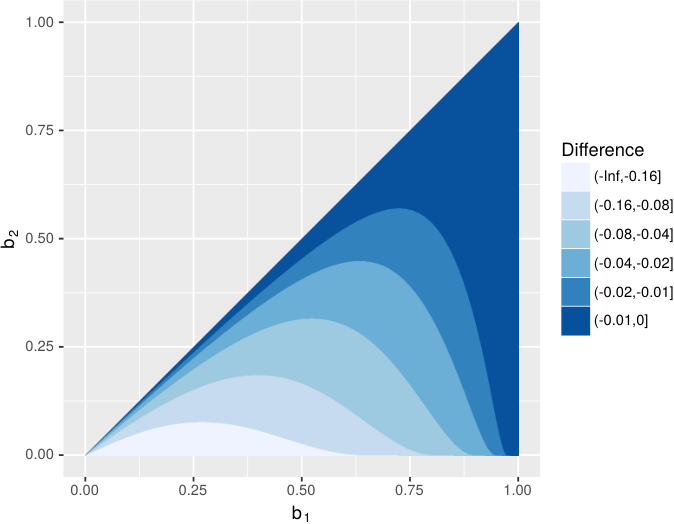
Data-Dependent Hamming LSH. The Hamming distance between two $t$-sparse vectors with Braun-Blanquet similarity $b$ is $2t(1-b)$, since the intersection of the vectors has size $tb$. This means that $(b_{1},b_{2})$-$B$-similarity search can be reduced to Hamming similarity search with approximation factor $c=(2t(1-b_{1}))/(2t(1-b_{2}))=(1-b_{1})/(1-b_{2})$. As mentioned above, the data dependent LSH technique of (Andoni and Razenshteyn, 2015) achieves $\rho=1/(2c-1)$ ignoring $o_{n}(1)$ terms. In terms of $b_{1}$ and $b_{2}$ this is $\rho_{\text{datadep}}=\frac{1-b_{1}}{1+b_{1}-2b_{2}}$, which in incomparable to the $\rho$ of Theorem 1.1. In Appendix B we show that $\rho<\rho_{\text{datadep}}$ whenever $b_{2}\leq 1/5$, or equivalently, whenever $j_{2}\leq 1/9$. Revisiting the above example, for $j_{1}=0.2$ and $j_{2}=0.1$ we have $\rho_{\text{datadep}}=0.6875$ which is about $0.043$ more than Chosen Path. Figure 5 gives a comparison covering the whole parameter space.

References

- Ahle et al. (2016) T. D. Ahle, R. Pagh, I. P. Razenshteyn, and F. Silvestri. 2016. On the Complexity of Inner Product Similarity Join. In Proc. PODS’16. 151–164.
- Andoni et al. (2015) A. Andoni, P. Indyk, T. Laarhoven, I. Razenshteyn, and L. Schmidt. 2015. Practical and optimal LSH for angular distance. In Proc. NIPS ’15. 1225–1233.
- Andoni et al. (2014) A. Andoni, P. Indyk, H. L. Nguyen, and I. P. Razenshteyn. 2014. Beyond Locality-Sensitive Hashing. In Proc. SODA ’14. 1018–1028.
- Andoni et al. (2017) A. Andoni, T. Laarhoven, I. P. Razenshteyn, and E. Waingarten. 2017. Optimal Hashing-based Time-Space Trade-offs for Approximate Near Neighbors. In Proc. SODA ’17. 47–66.
- Andoni and Razenshteyn (2015) A. Andoni and I. Razenshteyn. 2015. Optimal Data-Dependent Hashing for Approximate Near Neighbors. In Proc. STOC ’15. 793–801.
- Andoni and Razensteyn (2016) A. Andoni and I. Razensteyn. 2016. Tight Lower Bounds for Data-Dependent Locality-Sensitive Hashing. In Proc. SoCG ’16. 9:1–9:11.
- Arasu et al. (2006) Arvind Arasu, Venkatesh Ganti, and Raghav Kaushik. 2006. Efficient exact set-similarity joins. In Proceedings of the 32nd international conference on Very large data bases. VLDB Endowment, 918–929.
- Bayardo et al. (2007) Roberto J Bayardo, Yiming Ma, and Ramakrishnan Srikant. 2007. Scaling up all pairs similarity search. In Proceedings of the 16th international conference on World Wide Web. ACM, 131–140.
- Becker et al. (2016) A. Becker, L. Ducas, N. Gama, and T. Laarhoven. 2016. New directions in nearest neighbor searching with applications to lattice sieving. In Proc. SODA ’16. 10–24.
- Braun-Blanquet (1932) Josias Braun-Blanquet. 1932. Plant sociology. The study of plant communities. McGraw-Hill.
- Broder (1997) Andrei Z. Broder. 1997. On the resemblance and containment of documents. In Compression and Complexity of Sequences 1997. Proceedings. IEEE, 21–29.
- Broder et al. (1997) Andrei Z. Broder, Steven C. Glassman, Mark S. Manasse, and Geoffrey Zweig. 1997. Syntactic clustering of the web. Computer Networks and ISDN Systems 29, 8 (1997), 1157–1166.
- Charikar (2002) M. Charikar. 2002. Similarity estimation techniques from rounding algorithms. In Proc. STOC ’02. 380–388.
- Chierichetti and Kumar (2015) F. Chierichetti and R. Kumar. 2015. LSH-Preserving Functions and Their Applications. J. ACM 62, 5 (2015), 33.
- Choi et al. (2010) S. Choi, S. Cha, and C. C. Tappert. 2010. A survey of binary similarity and distance measures. J. Syst. Cybern. Informatics 8, 1 (2010), 43–48.
- Christiani (2017) T. Christiani. 2017. A Framework for Similarity Search with Space-Time Tradeoffs using Locality-Sensitive Filtering. In Proc. SODA ’17. 31–46.
- Cohen (1997) E. Cohen. 1997. Size-estimation framework with applications to transitive closure and reachability. J. Comp. Syst. Sci. 55, 3 (1997), 441–453.
- Cohen and Kaplan (2009) E. Cohen and H. Kaplan. 2009. Leveraging discarded samples for tighter estimation of multiple-set aggregates. ACM SIGMETRICS Performance Evaluation Review 37, 1 (2009), 251–262.
- Dubiner (2010) M. Dubiner. 2010. Bucketing coding and information theory for the statistical high-dimensional nearest-neighbor problem. IEEE Trans. Information Theory 56, 8 (2010), 4166–4179.
- Hagerup (1998) T. Hagerup. 1998. Sorting and Searching on the Word RAM. In Proc. STACS ’98. 366–398.
- Har-Peled et al. (2012) S. Har-Peled, P. Indyk, and R. Motwani. 2012. Approximate Nearest Neighbor: Towards Removing the Curse of Dimensionality. Theory of computing 8, 1 (2012), 321–350.
- Hoeffding (1963) W. Hoeffding. 1963. Probability inequalities for sums of bounded random variables. Jour. Am. Stat. Assoc. 58, 301 (1963), 13–30.
- Indyk and Motwani (1998) P. Indyk and R. Motwani. 1998. Approximate nearest neighbors: towards removing the curse of dimensionality. In Proc. STOC ’98. 604–613.
- Laarhoven (2015) T. Laarhoven. 2015. Tradeoffs for nearest neighbors on the sphere. CoRR abs/1511.07527 (2015). http://arxiv.org/abs/1511.07527
- Li and König (2011) Ping Li and Arnd Christian König. 2011. Theory and applications of b-bit minwise hashing. Commun. ACM 54, 8 (2011), 101–109.
- Mitzenmacher et al. (2014) M. Mitzenmacher, R. Pagh, and N. Pham. 2014. Efficient estimation for high similarities using odd sketches. In Proc. WWW ’14. 109–118.
- Mitzenmacher and Upfal (2005) M. Mitzenmacher and E. Upfal. 2005. Probability and computing. Cambridge University Press, New York, NY.
- Motwani et al. (2007) R. Motwani, A. Naor, and R. Panigrahy. 2007. Lower Bounds on Locality Sensitive Hashing. SIAM J. Discrete Math. 21, 4 (2007), 930–935.
- Motwani and Raghavan (2010) Rajeev Motwani and Prabhakar Raghavan. 2010. Randomized algorithms. Chapman & Hall/CRC.
- O’Donnell et al. (2014) R. O’Donnell, Y. Wu, and Y. Zhou. 2014. Optimal lower bounds for locality-sensitive hashing (except when q is tiny). ACM Transactions on Computation Theory (TOCT) 6, 1 (2014), 5.
- Pagh et al. (2014) Rasmus Pagh, Morten Stöckel, and David P Woodruff. 2014. Is min-wise hashing optimal for summarizing set intersection?. In Proceedings of the 33rd ACM SIGMOD-SIGACT-SIGART symposium on Principles of database systems. ACM, 109–120.
- Panigrahy et al. (2010) R. Panigrahy, K. Talwar, and U. Wieder. 2010. Lower Bounds on Near Neighbor Search via Metric Expansion. In Proc. FOCS ’10. 805–814.
- Shrivastava and Li (2015) Anshumali Shrivastava and Ping Li. 2015. Asymmetric minwise hashing for indexing binary inner products and set containment. In Proceedings of the 24th International Conference on World Wide Web. ACM, 981–991.
- Terasawa and Tanaka (2007) K. Terasawa and Y. Tanaka. 2007. Spherical LSH for Approximate Nearest Neighbor Search on Unit Hypersphere. In Proc. WADS ’07. 27–38.
- Thorup (2013) Mikkel Thorup. 2013. Bottom-k and priority sampling, set similarity and subset sums with minimal independence. In Proceedings of the forty-fifth annual ACM symposium on Theory of computing. ACM, 371–380.
- Topsœ (2007) F. Topsœ. 2007. Some Bounds for the Logarithmic Function. Vol. 4. Nova Science, 137–151.
- Zobrist (1970) Albert L Zobrist. 1970. A new hashing method with application for game playing. ICCA journal 13, 2 (1970), 69–73.