Adiabatic pumping solutions in global AdS

Quenching a system is a way of probing its dynamics. Relevant information can be collected by studying the way the system responds and relaxes. This concerns time-dependent processes that in general have to be tackled with numerical simulations. Nevertheless, taking some specific limits allows to capture significant features without very much computational cost. Recently, the limit of fast quenches has been under intense survey allowing to extract interesting scaling relations (see [1] and references therein). In the present paper we want to study the opposite limit, where considerable simplifications occur as well: pumping solutions are very simple configurations of the Einstein-scalar theory were the real massless scalar field has a constantly increasing source at the boundary.

From the AdS/CFT perspective the pumping solutions are dual to an eternally monotonically driven conformal field theory. Actually, although being strictly speaking a time dependent setup, the metric solution is perfectly static; technically this is related to the fact that, in the massless case, the metric couples to the scalar field only derivatively. From the $d$-dimensional boundary theory viewpoint, the masslessness of the bulk scalar implies that the dual theory is monotonically deformed by means of a marginal coupling.

In this paper we will work in the context of global AdS. For the planar situation, instead, one should first cure the infrared of the theory, and some considerations in the slow quench limit have been explored in [2] using the so called hard wall model. We find agreement with them in the existence of a maximum value for the driving time slope $\alpha_{b}$ and qualify this statement with some additional analysis.

The present paper is organized in five sections. In Section 1 we describe the stationary pumping ansatz and the equations to be solved. We pause to clarify the difference of parameterizing the space of solutions in the origin-time or the boundary-time gauge. We describe the space of solutions and obtain their energy density. This brings us to Section 2, where stability will be the main concern, both at the linear and the nonlinear level. The former study is straightforward and neat, the latter is more articulate and brings in some interesting properties like limiting cycles. Motivated by these oscillatory behaviors we search for and find time-periodic solutions, which we construct both perturbatively and numerically in Section 3. These periodic solutions branch continuously from their analogs in the pure AdS geometry [3]. In Section 4 we address the question of having a negative mass. We show that this effect is intimately tied to the fact that the scalar coupling rises linearly in time. Quenching back to a constant value for the scalar source restores the positivity of $m$. Section 5 focuses on the pumping solution over AdS₃ where, as usual, analytical control is much more attainable than in higher dimensions. In fact we provide a web of maps that links the pumping solution to a set of known models in the literature. Notably this includes magnetic horizonless and regular as well as translationally-breaking solutions. This mapping proves to be extremely useful, allowing for an exchange of explicit results from one model to the other. In particular, in this way an analytical pumping solution is obtained. We close the paper with some supplementary material linking the new solution to those encountered in seemingly very different contexts. In Appendix A, we generalize the results of Section 5 to higher dimensions. At the level of the equations of motion, they are shown to be derivable from a static magnetic $d$-form source. Appendix B, intended for the specialized reader, provides technical material containing details of the numerical construction of time-periodic pumping solutions. Finally in Appendix C we discuss a possible tension of the pumping solution with respect to entanglement inequalities. We comment some caveats that need to be elucidated.

Let us consider a real massless scalar field coupled to gravity plus a negative cosmological constant in $d+1$ dimensions

$$S=\int d^{d+1}x\sqrt{g}\left(\frac{1}{2\kappa^{2}}(R-2\Lambda)-\frac{1}{2}\partial_{\mu}\phi\partial^{\mu}\phi\right)\,,$$

(2.1)

with $\Lambda=-d(d-1)/2l^{2}$. Hereafter we will set $l=1$, $\kappa^{2}=d-1$ and fix the metric ansatz according to the following expression

$$ds^{2}=\frac{1}{\cos^{2}\!x}\left(-fe^{-2\delta}dt^{2}+f^{-1}dx^{2}+\sin^{2}\!x\,d\Omega_{d-1}^{2}\right)\,,$$

(2.2)

where the radial coordinate spans $x\in[0,\pi/2)$ and all fields are, a priori, functions of $t$ and $x$. The equations of motion for the scalar field can be cast in terms of the fields $\Phi=\phi^{\prime}$ and $\Pi=\dot{\phi}e^{\delta}/f$ as follows

$$\dot{\Phi}=\left(fe^{-\delta}\Pi\right)^{\prime}\penalty\ \penalty\ \penalty\ ;\penalty\ \penalty\ \penalty\ \dot{\Pi}=\displaystyle\frac{1}{\tan^{d-1}x}\left(\tan^{d-1}xfe^{-\delta}\Phi\right)^{\prime}\,.$$

(2.3)

From the Einstein equation we obtain just constraints

	$\displaystyle\delta^{\prime}$	$\displaystyle=$	$\displaystyle-\displaystyle\sin x\cos x\left(\Phi^{2}+\Pi^{2}\right)\,,$		(2.4)
	$\displaystyle f^{\prime}$	$\displaystyle=$	$\displaystyle\displaystyle\frac{d-2+2\sin^{2}\!x}{\sin x\cos x}(1-f)+\delta^{\prime}f\,.\rule{0.0pt}{22.76219pt}$		(2.5)

For $d\geq 3$, regularity of the Frobenius expansion close to the center of AdS_d+1 gives¹¹ 1 In $d=2$ the field $f$ may have an arbitrary value $f_{0}\in{\mathbb{R}}$ at the origin.

	$\displaystyle\phi(t,x)$	$\displaystyle=$	$\displaystyle\tilde{\phi}_{0}(t)+\tilde{\phi}_{2}(t)x^{2}+...\ ,$
	$\displaystyle\delta(t,x)$	$\displaystyle=$	$\displaystyle\tilde{\delta}_{0}(t)+\tilde{\delta}_{2}(t)x^{2}+...\ ,$		(2.6)
	$\displaystyle f(t,x)$	$\displaystyle=$	$\displaystyle 1+\tilde{f}_{2}(t)x^{2}+...\ .$

Performing a similar expansion in $d=3$ for $x\to\pi/2$ and defining $\rho=\frac{\pi}{2}-x$, leads to the boundary series expansion²² 2 Note that for even $d$ the expansions contain in general logarithmic terms as well.

	$\displaystyle\phi(t,x)$	$\displaystyle=$	$\displaystyle\phi_{0}(t)+\phi_{2}(t)\rho^{2}+\phi_{3}(t)\rho^{3}+...\penalty\ \penalty\$
	$\displaystyle\delta(t,x)$	$\displaystyle=$	$\displaystyle\delta_{0}(t)+\delta_{2}(t)\rho^{2}+...\penalty\ \penalty\ ,$
	$\displaystyle f(t,x)$	$\displaystyle=$	$\displaystyle 1+f_{2}(t)\rho^{2}+f_{3}(t)\rho^{3}+...$		(2.7)

In this boundary expansion, every time-dependent coefficient is a functional of $\phi_{0}(t)$, $\phi_{3}(t)$, $\delta_{0}(t)$ and $f_{3}(t)$. In the AdS/CFT dictionary, $\phi_{0}(t)$ is dual to the QFT source, while $\phi_{3}(t)$ is proportional to the vev $\langle{\cal O}_{\phi}\rangle$. Performing a coordinate change to bring the line element (2.2) to the standard Fefferman-Graham form $ds^{2}=\frac{dz^{2}}{z^{2}}+\frac{g_{ab}(z,t,x)}{z^{2}}dx^{a}dx^{b}$ and expanding $g_{ab}(z,t,x)=\eta_{ab}+...+z^{3}t_{ab}+...$ we can read off the value of the energy density $m\equiv\left<T_{tt}\right>=-1/2f_{3}$. Furthermore, the Ward identity associated to time translations reads³³ 3 These statements rely on the holographic renormalization of the model which is commented briefly at the end of this section.

$$\partial_{t}\left<T_{tt}\right>=-\partial_{t}\phi_{0}\langle{\cal O}_{\phi}\rangle\,.$$

(2.8)

In order to look for background solutions, we plug the stationary ansatz $\dot{\Pi}=\dot{\Phi}=\dot{f}=\dot{\delta}=0$ in (2.3), and obtain the following constraints depending upon two integration constants $\alpha$ and $\beta$

$$\Pi=\frac{\alpha e^{\delta}}{f}\ ,\qquad\Phi=\frac{\beta e^{\delta}}{f\tan^{d-1}\!x}\,.$$

(2.9)

From the near origin expansion (2.6) it directly follows that $\beta=0$, hence $\Phi=\phi^{\prime}=0$ for all times. There exists a symmetry of (2.9) under $\delta\to\delta-a$ and $\alpha\to\alpha\,e^{a}$ that is the unbroken remnant, $t\to e^{-a}t$, of the group of time diffeomorphisms. Tuning $a$ allows to select the position $x_{p}$ where $\delta(t,x_{p})=0$. We consider now the boundary time gauge choice, $x_{p}=\pi/2$, which is tantamount to setting $\delta_{0}(t)=0$ in the near-boundary expansion (2.7).

We are interested in solutions characterized by a linearly rising source $\phi_{0}(t)=\alpha_{b}t$ where $t\in{\mathbb{R}}$. In the boundary time gauge, $t=t_{b}$, these sourced solutions are the natural dual to a QFT observer performing continuous quenches. $\alpha_{b}$ is the pumping strength, and the label stresses the fact that its definition is linked to the boundary time gauge, where in addition one has $\Pi(t,\pi/2)=\alpha=\alpha_{b}$.

Inserting $\Pi$ and $\Phi=0$ into (2.4) and (2.5) we get a simple system to be solved for $f$ and $\delta$, namely

	$\displaystyle\delta_{b}^{\prime}$	$\displaystyle=$	$\displaystyle-\displaystyle\frac{\alpha_{b}^{2}\sin x\cos xe^{2\delta_{b}}}{f^{2}},$		(2.10)
	$\displaystyle f^{\prime}$	$\displaystyle=$	$\displaystyle\displaystyle\frac{d-2+2\sin^{2}\!x}{\sin x\cos x}(1-f)+\delta_{b}^{\prime}f\,.\rule{0.0pt}{22.76219pt}$		(2.11)

In $d=2$ these equations admit an analytic solution, while for $d\geq 3$ they must be solved numerically. We will discuss the $d=3$ case from now on. We consider the boundary conditions $\delta(\pi/2)=0$, $f(\pi/2)=1$ and find that the equations can only be solved for $\alpha_{b}\leq\alpha_{b,max}$. In this sense, $\alpha_{b,max}$ corresponds to an intrinsic adiabaticity threshold present in our system. Here the concept of adiabaticity threshold refers to the fact that the source should grow slowly enough (with respect to the scale set by the $AdS$ radius, $\alpha_{b}^{-1}>\pi$) in order for the system to be able to keep up with it. Solutions with faster growth are either non-regular or non-static, typically collapsing into a black hole. In the following sections we further study this key point.

Actually, the story is slightly subtler. It turns out that $\alpha_{b}$ is not a faithful parameter. Instead, it will be convenient to shift momentarily to the origin time gauge choice, where the time coordinate coincides with the proper time at the origin, $t=t_{o}$. The equations look exactly the same as (2.10) and (2.11) replacing $\delta_{b}\to\delta_{o}$ and $\alpha_{b}\to\alpha_{o}$. The boundary condition to solve them now involves instead $\delta_{o}(x=0)=0$. It is clear that, in this gauge $\alpha_{o}=\Pi(x=0)$. Remarkably, it turns out that, for any value of $\alpha_{o}\in[0,\infty)$ there exists a stationary solution with vanishing $\langle{\cal O}_{\phi}\rangle$ and constantly rising scalar field $\phi(t)=\alpha_{o}t_{o}=\alpha_{b}t_{b}$. In Fig.1 we plot a family of solutions for regularly spaced values of $\alpha_{0}\in[0,20]$. The tension between the two parameterizations is resolved because the mapping $\alpha_{o}\to\alpha_{b}(\alpha_{o})$ is not everywhere one-to-one. Actually, it has a maximum at $(\alpha_{o,{\rm thr}},\alpha_{b,{\rm max}})=(2.01,0.785)$. This can be clearly seen in the left plot of Fig.2.

Let us pause here an discuss why the existence of the pumping solutions is remarkable. On general grounds, the pumping source $\phi_{0}(t)=\alpha t$ is expected to be associated with a process of energy injection that leads to a time-dependent geometry that eventually may collapse gravitationally. However, the Ward identity (2.8) readily implies that, if the pumping source is accompanied by a vanishing vev, $\left<\mathcal{O}_{\phi}(t)\right>=0$, the energy density remains constant, $\dot{m}(t)=0$. This is precisely the situation in the pumping solution, since $\Phi(t,x)=0$. Notice that the physical mechanism behind the existence of the pumping solutions could also be the reason of its physical irrelevance: the question of whether the pumping solution background is infinitely fine-tuned, in the sense that it is destroyed by any infinitesimal perturbation such that $\Phi(t,x)\neq 0$, needs to be explicitly addressed.

In fact, we can compute the energy density of the pumping solutions, and perform two important observations (see Fig.2, left). The first one is that there exist a threshold value $\alpha_{o,1}$ such that, for $\alpha_{o}<\alpha_{o,1}$, $m$ is negative. Similarly to other gravitational backgrounds with negative mass, this raises a concern regarding stability [4]. The second one is that there exists yet another threshold value $\alpha_{o,2}>\alpha_{o,1}$ where the energy density curve $m(\alpha_{0})$ reaches an extremum. We may naively think that $\alpha_{o,2}$ implies the appearance of a Chandrasekhar instability. Both issues will be discussed in the next section.

The identification of $f_{3}$ with the energy density $m$ relies as usual on a holographic renormalization program, including finite counter-terms. Although the full holographic renormalization of the time-dependent model is beyond the scope of the present analysis, we have checked that this identification is not affected in the present setup. Indeed, despite the breaking of time translations by the background, the counter-terms must be invariant combinations of the induced fields on the boundary cutoff surface. Their invariance is referred to the transverse diffeomorphisms. The only new counter-term which could affect the renormalized on-shell action linear in the fluctuations (i.e. that could affect the definition of the energy density and the 1-point Ward identities) is proportional to $\sqrt{-\gamma}(\partial_{\mu}\phi)(\partial^{\mu}\phi)$, where $\gamma$ is the induced metric on the boundary. Nevertheless, relying on the structure of the asymptotic near-boundary expansions of the fields, it is possible to show that such counter-term does not contribute at the finite level.⁴⁴ 4 For a treatment of the holographic renormalization of massless scalars we refer in particular to [5]. Given the technical and conceptual connection of the present model with those breaking spatial translations, it is useful to relate the holographic renormalization in these two contexts, see [6].

In order to connect two infinitesimally close pumping solutions through a normalizable fluctuation, one needs $\alpha_{b}^{\prime}(\alpha_{o})=0$. Notice that this occurs at $\alpha_{o}=\alpha_{o,\text{thr}}$ and not at $\alpha_{o}=\alpha_{0,2}$ (where instead it is the mass which attains its maximal value). We recall that $\alpha_{b,\text{max}}$ corresponds to $\alpha_{o,\text{thr}}$. For linearized fluctuations around the pumping solution contained in our original ansatz, an explicit computation shows that, indeed, at $\alpha_{b}=\alpha_{b,\textrm{max}}$, a zero mode appears in the eigenfrequency spectrum (see Fig.2, right). Therefore, pumping solutions with $\alpha_{o}>\alpha_{o,\textrm{thr}}$ are linearly unstable. This entails that, in principle, only pumping solutions with $\alpha_{o}\leq\alpha_{o,\textrm{thr}}$ can be prepared by a quasistatic quench starting from the AdS₄ vacuum.

Two questions naturally arise at this point. The first one is whether the linear stability of the $\alpha_{o}\leq\alpha_{o,\textrm{max}}$ pumping solutions translates into nonlinear stability. The second one concerns the final state reached by the $\alpha_{o}>\alpha_{o,\textrm{thr}}$ pumping solutions once perturbed.

Let us address the first question. Notice first that, by virtue of the Ward identity (2.8), even if a linear eigenmode has a nonzero $\left<\mathcal{O}_{\phi}(t)\right>$, since its time dependence is harmonic, the energy density it generates would also oscillate periodically with a $\pi/2$ phase shift with respect to $\left<\mathcal{O}_{\phi}(t)\right>$. Nonlinear perturbations, being generically nonharmonic, might trigger a nonlinear instability due to the existence of a finite $\Phi(t,x)$ with generic time dependence, that can lead to an energy exchange eventually resulting in a gravitational collapse. There exist two complementary ways of establishing the absence of potential nonlinear instability. The first one is realizing that pumping solutions below $\alpha_{o,\textrm{thr}}$ can be actually accessed through a quasistatic quench. Indeed, we have simulated the time-dependent geometry generated by a source $\phi_{0}(t)$ such that $\phi_{0}(t<0)=0$, $\ddot{\phi_{0}}/\dot{\phi_{0}}^{2}\ll 1$ and $\lim_{t\to\infty}\phi_{0}/t=\alpha_{b}$, and have checked that, at sufficiently late times, it settles down into the linearly stable pumping solution corresponding to $\alpha_{b}$ (see Fig.8 in Section 5). In consequence, the pumping solutions play an important role at the nonlinear level: were they subjected to nonlinear instability, the system would never relax to them.

The second approach we followed in order to determine whether linearly stable pumping solutions are also nonlinearly stable was to take, as initial data at $t=0$,

	$\displaystyle\Phi(0,x)=0,$		(3.1)
	$\displaystyle\Pi(0,x)=\Pi_{\alpha_{o}}(x)+\frac{2\epsilon}{\pi}\exp\left(-\frac{4\tan^{2}x}{\pi^{2}\sigma^{2}}\right)\,,$		(3.2)

and simulate their subsequent time evolution. $\Pi_{\alpha_{o}}(x)$ represents a pumping solution characterized by $\alpha_{o}$. An example is depicted in Fig.3, for $\alpha_{o}=1$, $\epsilon=1$ and $\sigma=0.1$. Due to the Gaussian perturbation, the initially negative $m(0)$ does not remain constant: its time derivative perfectly satisfies the Ward identity (2.8) in the presence of the nontrivial $\left<\mathcal{O}_{\phi}\right>$ that is generated. Both quantities, $m(t)$ and $\left<\mathcal{O}_{\phi}(t)\right>$, are found to oscillate in a disordered way around their respective initial values. In fact, we find that the time-averaged energy density, $\left<m\right>=t^{-1}\int_{0}^{t}m(t^{\prime})dt^{\prime}$, rapidly reaches a constant value and the system absorbs/loses no net energy density. Therefore, no sign of nonlinear instability is found.

The endpoint of the unstable pumping branch for $\alpha_{o}<\alpha_{o,c}$ is, as said before, a limiting cycle. For $0<\alpha_{o}-\alpha_{o,{\rm thr}}\ll 1$ this limiting cycle has a single period. This fact came as unexpected, and prompted us to look for exactly periodic solutions with a pumping source. Time-periodic solutions in global AdS supported by a real massless scalar field with zero source were originally presented in [3] and we now show that, for $\alpha_{b}\neq 0$,⁶⁶ 6 For small $\alpha_{o}$ we can equally use $\alpha_{b}$ as deformation parameter since the relation that links them is one-to-one. each such solution generalizes into a family of exactly periodic pumping solutions. The existence of pumping time-periodic solutions can be first proved at the perturbative level and later corroborated with a numerical approach.

Let $\Omega$ be the frequency of the periodic solution we aim at.⁷⁷ 7 Recall that scalar eigenmodes in global AdS have a frequency spectrum given by $\omega_{n}=\Delta+2n$, where $\Delta$ is the conformal dimension of the dual scalar operator. For a massless scalar field in AdS₄, $\Delta=3$. Rescale the time coordinate as $\tau\equiv\Omega\,t$ and introduce the following ansatz

	$\displaystyle\phi(\tau,x)=\alpha_{b}\frac{\tau}{\Omega(\alpha_{b},\epsilon)}+\epsilon\cos^{3}\!x\sin\tau+\sum_{n=1}^{\infty}\sum_{k=0}^{2n+1}\varphi_{2n+1-k,k}(\tau,x)\alpha_{b}^{2n+1-k}\epsilon^{k},$		(4.1)
	$\displaystyle\delta(\tau,x)=\sum_{n=1}^{\infty}\sum_{k=0}^{2n}d_{2n-k,k}(\tau,x)\alpha_{b}^{2n-k}\epsilon^{k},\penalty\ f(\tau,x)=1+\sum_{n=1}^{\infty}\sum_{k=0}^{2n}a_{2n-k,k}(\tau,x)\alpha_{b}^{2n-k}\epsilon^{k},$		(4.2)
	$\displaystyle\Omega(\alpha_{b},\epsilon)=3+\sum_{n=1}^{\infty}\sum_{k=0}^{2n}\omega_{2n-k}\alpha_{b}^{2n-k}\epsilon^{k}.$		(4.3)

At first order in $\alpha_{b}$ and $\epsilon$ we are just considering the linear superposition of the pumping solution $\phi_{\alpha}(t,x)=\alpha_{b}t$ and the fundamental eigenmode of the scalar field $\phi_{\epsilon}=\epsilon\sin\tau\cos^{3}\!x$ over global AdS₄. Higher order corrections determine how the seed $\phi_{\alpha}+\phi_{\epsilon}$ is dressed nonlinearly. The interested reader can find a thorough discussion with technical details in Appendix B. For our present purposes it suffices to mention that, after the first nonlinear correction, the seed frequency $\Omega_{0}=3$ is modified to

$$\Omega=\Omega_{0}-\frac{135}{128}\epsilon^{2}-\frac{7}{4}\alpha_{b}^{2}.$$

(4.4)

To close the gap between the perturbative and the fully nonlinear regime, one needs to resort to numerical methods. In particular, since the eigenmodes of the AdS₄ Laplacian do not satisfy the boundary conditions (2.7),⁸⁸ 8 A finite mass breaks the parity under $\rho\to-\rho$ that the scalar field near-boundary expansion exhibits at the linearized level. we have adapted the pseudospectral method described in [8] to our present setup.

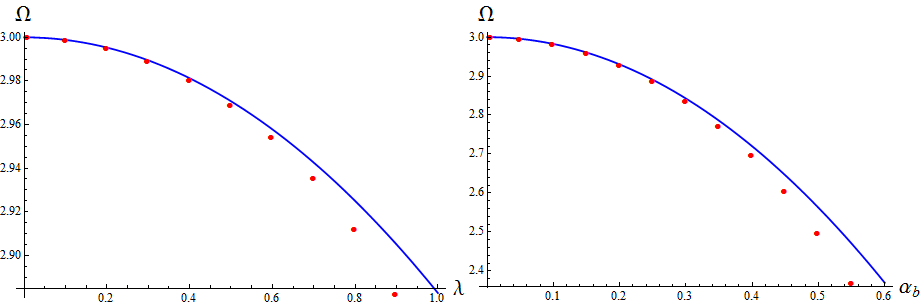
Let us perform two different checks on the periodic solutions found numerically. We define $\lambda$ as the value of the vev at $\tau=\pi/2$, $\lambda\equiv\left<\mathcal{O}_{\phi}(\tau=\pi/2)\right>=3\epsilon$. In Fig.6, we plot $\Omega(\alpha_{b},\lambda)$ for two orthogonal directions in the phase space of exactly periodic solutions, and compare it with (4.4). In each case, excellent agreement is found between the perturbative and the numerical result in the $\alpha_{b},\epsilon\ll 1$ regime.

As a further consistency check, we perform a simulation starting from $\Pi(t=0,x)=\Pi_{0}(x)$ and $\Phi(t=0,x)=0$ as determined by the pseudospectral algorithm and study their subsequent time evolution. We provide one example in Fig.7. It is observed that the time development of the initial data perfectly agrees with the output of the pseudospectral code, providing a highly nontrivial check of our numerical procedures.

We have already mentioned that all pumping states with $\alpha_{b}\leq\alpha_{b,{\rm max}}$ can be prepared by a boundary quasistatic quench$\alpha_{b}(t)$. Notice that the stability analysis in Section 3 was restricted to isotropic perturbations. We have seen that the fact that the pumping solution has energy density below that of AdS is not associated to an instability for small values of $\alpha_{o}$.

A nice consequence of this is the fact that the pumping solution with negative mass can be obtained by means of a quench that starts from the AdS vacuum, $\alpha_{b}=0$, and ramps this slope quasistatically to some $0<\alpha_{b}<\alpha_{b,max}$. This can be observed in the first part of Fig.8, where the pumping solution is the mid part ($100<t<300$). This experimental way of building the pumping solution illustrates also the meaning of the adiabadicity threshold. Indeed, ramping $\alpha_{b}$ beyond the value $\alpha_{b,max}=0.783$ leads immediately to sudden black hole formation. In other words, there is no way to explore the region beyond $\alpha_{b,max}$ by means of an experimental quench. We also want to remind the reader that all the solutions that in Fig.2 lie to the right of the maximum of the blue curve are eternal and only exist as solutions to the static equations.
Turning back to the issue of the possible puzzle with having a stable static solution with negative mass, a numerical experiment is at the same time clarifying and intriguing. Starting from a pumping solution with negative mass, like the one in Fig.8 at intermediate times ($100<t<300$), we can think of suddenly isolating the system from the environment by switching off the scalar source. Naively, from the Ward identity, no energy inflow can occur and one would think that, in this way, we end up with a a regular stationary solution of negative mass. However, this does not happen. Turning off the pumping can be achieved by stopping the linear growth of $\phi_{0}$ as some time $t_{f}$. In practice, this has to be implemented through a smooth interpolation of time span $\delta$ between the pumping boundary condition $\dot{\phi}_{0}(t<t_{f}-\delta/2)=\alpha_{b}$ and a constant final value $\dot{\phi}_{0}(t>t_{f}+\delta/2)=0$ in the limit $\delta\to 0$. The remarkable result is that, for any value of $\delta$ and any interpolation used, the solution always returns to a positive energy density $m>0$ at times $t>t_{f}+\delta$. In fact, for an extremely wide and smooth interpolation, the final configuration attained is the static AdS₄ background with $m=0$.

For more abrupt interpolations the eventual geometry is time-dependent with a constant positive mass $m>0$. An example for $\delta=0.1$ can be seen in Fig.8. At late times, the final fate of this evolution encounters the issue of stability of a scalar pulse evolving in global AdS₄. In fact, if we consider the limit $\delta\to 0$, the energy density peaks so violently that a direct collapse may occur immediately after $t_{f}$.

Let us analyze the above mentioned behavior in detail. In Fig.9, we plot $m(\delta)$ and $\textrm{max}_{t\in[0,\delta]}\left<\mathcal{O}_{\phi}(t)\right>$ for a quench off the $\alpha_{o}=1$ pumping solution with the interpolating function

$$\dot{\phi}_{0}(t)=\frac{1}{2}\alpha_{b}\left[1+\tanh\left(\frac{\delta}{t}+\frac{\delta}{t-\delta}\right)\right]\qquad,\qquad t\in[0,\delta].$$

(5.1)

For $\delta\lesssim 1$, both $m(\delta)$ and $\textrm{max}_{t\in[0,\delta]}\left<\mathcal{O}_{\phi}(t)\right>$ display a well defined scaling with respect to $\delta$, $m(\delta)\propto\delta^{-1}$ and $\textrm{max}_{t\in[0,\delta]}\left<\mathcal{O}_{\phi}(t)\right>\propto\delta^{-2}$, confirming that both diverge in the $\delta\to 0$ limit.

A natural question is if the observed scaling is related to the fact that we are quenching off the pumping solution, or is rather determined by the particular form of the interpolating function (5.1). To answer this question, in Fig.10 we plot $m(\delta)$ and $\textrm{max}_{t\in[0,\delta]}\left<\mathcal{O}_{\phi}(t)\right>$ for a quench with $\phi_{0}(t)$ given by the time-reversed version of (5.1) acting over the AdS₄ vacuum,

$$\dot{\phi}_{0}(t)=\frac{1}{2}\alpha_{b}\left[1-\tanh\left(\frac{\delta}{t}+\frac{\delta}{t-\delta}\right)\right]\qquad,\qquad t\in[0,\delta].$$

(5.2)

We observe that the former scaling relations $m(\delta)\propto\delta^{-1}$, $\textrm{max}_{t\in[0,\delta]}\left<\mathcal{O}_{\phi}(t)\right>\propto\delta^{-2}$ uphold, showing that the scaling is solely determined by the precise non-analytic behavior of the source in the $\delta\to 0$ limit: both (5.1) and (5.2) result in quench profiles $\phi_{0}(t)$ that are continuous but non-differentiable.

The scaling displayed by $m(\delta)$ and $\textrm{max}_{t\in[0,\delta]}\left<\mathcal{O}_{\phi}(t)\right>$ under (5.2) differs from the one that would be present if the quenching profile (5.2) were considered on $\phi_{0}(t)$, rather than on $\dot{\phi}_{0}(t)$. In the case of a $\phi_{0}(t)$ fast quench, the scaling relations are $m(\delta)\propto\delta^{-3}$ and $\textrm{max}_{t\in[0,\delta]}\left<\mathcal{O}_{\phi}(t)\right>\propto\delta^{-3}$, as expected on purely dimensional grounds [9]. We plot representative results of this behavior in Fig.11.

These numerical experiments confirm that no negative mass will be measured by a boundary observer when the source has settled to a constant value. It rises therefore the question about the nature of the quantum state dual to the pumping geometry. Is it really a bona fide quantum state? We will see in Appendix C that further information coming from entropy inequalities may cast some further shadows on this.

As a further observation, note that the whole process of quenching in and off embodies some irreversible character. Imagine slowly building up the value of $\alpha_{b}(t)$ from zero to a constant final value in a time span $\delta$, staying there for a long time, and finally switching back $\alpha_{b}(t)\to 0$ using the same $\delta$-smeared step function, but time reversed. Even if both the equations of motion and the boundary conditions are time reversal invariant, the end result will always have $m(t=\infty)\geq m(t=0)=0$, and only $m(t=\infty)=0$ in the quasistatic limit $\delta\to\infty$ for both steps.

In this section we shall investigate the three dimensional case. It turns out that the pumping solution over AdS₃ is related to a number of other solutions known in the literature via a series of mappings that includes double Wick rotations and/or Hodge dualities. This observation allows us to give an analytic expression for the pumping solution.

Let us consider a three-dimensional charged black brane with negative cosmological constant [10, 11]. The metric and the electromagnetic potential are given by

	$\displaystyle ds^{2}$	$\displaystyle=$	$\displaystyle-h(r)dt^{2}+\frac{dr^{2}}{h(r)}+r^{2}dx^{2},$		(6.1)
	$\displaystyle h(r)$	$\displaystyle=$	$\displaystyle r^{2}-M-Q_{e}^{2}\log(r),$		(6.2)
	$\displaystyle\rule{0.0pt}{17.07164pt}A(r)$	$\displaystyle=$	$\displaystyle\left[\mu-Q_{e}\log(r)\right]dt.$		(6.3)

In the expressions above, $r\in[0,\infty)$ and $t,x\in\mathbb{R}$. $M$ and $Q_{e}$ determine respectively the mass and the electric charge of the black brane geometry. From now on, we focus on the one-parameter family of charged black branes with $M=1$ and $\mu=0$. Note that the outer horizon is located at $r=r_{h}=1$ for $\left|Q_{e}\right|<\sqrt{2}$. The temperature is

$$T=\frac{1}{2\pi}\left(1-\frac{1}{2}Q_{e}^{2}\right).$$

(6.4)

At $\left|Q_{e}\right|=\sqrt{2}$ the black brane is extremal. For $\left|Q_{e}\right|>\sqrt{2}$, the hypersurface $r=1$ actually corresponds to the inner horizon, and (6.4) does not represent the real temperature of the back brane. By performing the coordinate change $r^{2}=1+R^{2}$, the exterior region of the charged black brane can be parameterized as

	$\displaystyle ds^{2}$	$\displaystyle=$	$\displaystyle-h(R)dt^{2}+\frac{R^{2}}{(1+R^{2})h(R)}dR^{2}+(1+R^{2})dx^{2},$		(6.5)
	$\displaystyle\rule{0.0pt}{17.07164pt}h(R)$	$\displaystyle=$	$\displaystyle R^{2}-\frac{1}{2}Q_{e}^{2}\log(1+R^{2}),$		(6.6)
	$\displaystyle\rule{0.0pt}{19.91692pt}A$	$\displaystyle=$	$\displaystyle-\frac{1}{2}Q_{e}\log(1+R^{2})dt.$		(6.7)

with $R\in[0,\infty)$. Now, let us perform the double Wick rotation defined by

$$t\to i\varphi,\penalty\ \penalty\ \penalty\ x\to it,\penalty\ \penalty\ \penalty\ \penalty\ Q_{e}\to-iQ_{m},$$

(6.8)

in a such a way that the geometry and electromagnetic potential of the exterior region are mapped to the following solution of three-dimensional Einstein-Maxwell theory with a negative cosmological constant

	$\displaystyle ds^{2}$	$\displaystyle=$	$\displaystyle-(1+R^{2})dt^{2}+\frac{R^{2}}{(1+R^{2})h(R)}dR^{2}+h(R)d\varphi^{2},$		(6.9)
	$\displaystyle h(R)$	$\displaystyle=$	$\displaystyle R^{2}+\frac{1}{2}Q_{m}^{2}\log(1+R^{2}),$		(6.10)
	$\displaystyle\rule{0.0pt}{19.91692pt}A$	$\displaystyle=$	$\displaystyle-\frac{1}{2}Q_{m}\log(1+R^{2})d\varphi.$		(6.11)

This is a horizonless geometry. It can be explicitly shown that the coordinate $\varphi$ must be identified with period $\beta=2\pi/(1+Q_{m}^{2}/2)$ in order to avoid a conical singularity at $R=0$. On the other hand, this period is nothing but the analytic continuation of the inverse temperature of the original charged black brane under the double Wick rotation. The geometry (6.9), (6.10) is supported by the radial magnetic field associated to (6.11), and we will refer to it as the magnetic AdS₃ solution.⁹⁹ 9 This background was originally found in references [12, 13, 14]. In [14], the authors introduced the double Wick rotation we discussed here. See [15, 16] for the construction of the general magnetic solution with angular momentum, the computation of its conserved charges and a proposed physical interpretation. The physical nature of the magnetic solution was further elucidated in [17].

We want to map the magnetic solution to the pumping solution. To this purpose we will rely on Hodge duality. However we have still to massage the magnetic solution: let us rescale our coordinates as $t\to\beta/(2\pi)t$, $R\to 2\pi/\beta R$ and $\varphi\to\beta/(2\pi)\varphi$, in such a way that $\varphi\sim\varphi+2\pi$.¹⁰¹⁰ 10 The rescaling of the $t$ and $R$ coordinates follows from the requirement that $\lim_{R\to\infty}R^{-2}ds^{2}=-dt^{2}+d\varphi^{2}$. This corresponds to the standard flat space metric as the representative of the conformal structure of the boundary where we have chosen $\Omega(R)=R^{-2}$ as conformal factor. Note also that this is the same procedure we would have employed were we on the vacuum state. In this new coordinate system, we have that

	$\displaystyle ds^{2}$	$\displaystyle=$	$\displaystyle-\left[\left(\frac{\beta}{2\pi}\right)^{2}+R^{2}\right]dt^{2}+\frac{R^{2}}{\left[\left(\frac{\beta}{2\pi}\right)^{2}+R^{2}\right]h(R)}dR^{2}+h(R)d\varphi^{2},$		(6.12)
	$\displaystyle\rule{0.0pt}{22.76219pt}h(R)$	$\displaystyle=$	$\displaystyle R^{2}+\frac{1}{2}\tilde{Q}_{m}^{2}\log\left[\left(\frac{\beta}{2\pi}\right)^{2}+R^{2}\right]+\tilde{\mu}\tilde{Q}_{m},$		(6.13)
	$\displaystyle\rule{0.0pt}{22.76219pt}A$	$\displaystyle=$	$\displaystyle-\left\{\tilde{\mu}+\frac{1}{2}\tilde{Q}_{m}\log\left[\left(\frac{\beta}{2\pi}\right)^{2}+R^{2}\right]\right\}d\varphi,$		(6.14)

where we have defined

$$\tilde{Q}_{m}\equiv\frac{\beta}{2\pi}Q_{m}=\frac{Q_{m}}{1+\frac{1}{2}Q_{m}^{2}}\,\qquad,\qquad\tilde{\mu}\equiv\tilde{Q}_{m}\log\frac{2\pi}{\beta}\ .$$

(6.15)

The field strength corresponding to the magnetic solution is

$$F=-\tilde{Q}_{m}\frac{R}{\left(\frac{\beta}{2\pi}\right)^{2}+R^{2}}\;dR\wedge d\varphi.$$

(6.16)

Under Hodge duality, the magnetic AdS₃ solution can be put into correspondence with the three-dimensional pumping solution. Recall that the vacuum Maxwell equations are $dF=d(\star F)=0$, where $\star$ is the Hodge operator. In three dimensions, the Hodge dual of a two-form corresponds to a one-form. Hence $F$ can be alternatively expressed as $F=\star d\phi$, where $\phi$ is a massless scalar field. The Bianchi identity $dF=0$ transforms into the scalar field equation of motion, $-\star d(\star d\phi)=\nabla^{2}\phi=0$, while the dynamical Maxwell equation reduces to the trivial statement $d^{2}\phi=0$. The map leaves the metric invariant and, as a consequence, a metric supported by a given electromagnetic field can be thought of as being sourced by the dual scalar field defined by this procedure.

Let us consider explicitly how the Hodge duality works at the level of the solution. Take the three-dimensional pumping solution with $\phi(t,r)=\alpha t$. Under Hodge duality, we find that the scalar field profile maps to

$$F=-\alpha\frac{re^{\delta(r)}}{f(r)}dr\wedge d\varphi,$$

(6.17)

where we have parameterized the pumping solution geometry in standard Schwarzschild coordinates,

$$ds^{2}=-f(r)e^{-2\delta(r)}dt^{2}+\frac{dr^{2}}{f(r)}+r^{2}d\varphi^{2}.$$

(6.18)

Note that the radial coordinates of the magnetic AdS₃ solution and the pumping solution are related by

$$r^{2}=h(R),$$

(6.19)

as it emerges from comparing the $\varphi\varphi$-component of the metric (6.9) and (6.18). From a comparison of the radial components of (6.9) and (6.18), we have that $r$ and $R$ must also satisfy

$$\frac{dr^{2}}{f(r)}=\frac{R^{2}dR^{2}}{\left[\left(\frac{\beta}{2\pi}\right)^{2}+R^{2}\right]h(R)}.$$

(6.20)

Deriving (6.19) and substituting into the expression above, we obtain the relation

$$f(r(R))=\left[\left(\frac{\beta}{2\pi}\right)^{2}+R^{2}\right]\left(1+\frac{1}{2}\frac{\tilde{Q}_{m}^{2}}{\left(\frac{\beta}{2\pi}\right)^{2}+R^{2}}\right)^{2}\ ,$$

(6.21)

where the explicit form of $h(R)$ provided by equation (6.13) has been employed. Note that, when $R=0$, (6.13) implies that $r=h(0)=0$. As a consequence, from (6.21) and the definitions of $\beta$ and $\tilde{Q}_{m}$, it follows that $f(0)=1$, a fact that shows the absence of a conical singularity at the origin in a manifest way.

By identifying now the $tt$-components of the metrics (6.9) and (6.18), we get that

$$\left(\frac{\beta}{2\pi}\right)^{2}+R^{2}=f(r)e^{-2\delta(r)}.$$

(6.22)

Employing equation (6.21), we finally obtain

$$\delta(r(R))=\log\left(1+\frac{1}{2}\frac{\tilde{Q}^{2}_{m}}{\left(\frac{\beta}{2\pi}\right)^{2}+R^{2}}\right).$$

(6.23)

Notice that $\delta(\infty)=0$, which means that the parametrization of the magnetic solution corresponds to the boundary time gauge (see Section 2).

With the help of equations (6.19), (6.21) and (6.23) we can express the field strength dual (in the Hodge sense) to the pumping solution in $R$ coordinates, namely

$$F=-\alpha\frac{R}{\left(\frac{\beta}{2\pi}\right)^{2}+R^{2}}\;dR\wedge d\varphi.$$

(6.24)

Comparing (6.24) with (6.16) we find that the pumping solution corresponds to a magnetic solution such that

$$\alpha=\tilde{Q}_{m}=\frac{Q_{m}}{1+\frac{1}{2}Q_{m}^{2}},$$

(6.25)

or, alternatively,

$$Q_{m}=\frac{1\pm\sqrt{1-2\alpha^{2}}}{\alpha}.$$

(6.26)

From (6.26), we have that the reality of $Q_{m}$ implies that $\left|\alpha\right|$ is restricted to the domain $\left|\alpha\right|\in\left[0,\frac{1}{\sqrt{2}}\right]$. Furthermore, a given $\alpha$ has two associated $Q_{m}$ parameters, $Q_{\pm}$, in a self-explaining notation. The $Q_{+}$ branch is restricted to the domain $\left|Q_{+}\right|\in[\sqrt{2},\infty)$, with limits respectively attained at $\left|\alpha\right|=1/\sqrt{2}$, $\alpha=0$. The $Q_{-}$ branch satisfies $\left|Q_{-}\right|\in[0,\sqrt{2}]$, and its limits correspond to $\alpha=0,\left|\alpha\right|=1/\sqrt{2}$. We observe that both branches merge at the critical value $\left|\alpha\right|=\alpha^{*}\equiv 1/\sqrt{2}$.

The two-branch structure of (6.26) is particularly interesting. Indeed, as we will show in the next subsection through an explicit computation, the $Q_{-}$ branch of magnetic solutions corresponds to the branch of linearly stable pumping solutions, while the $Q_{+}$ branch maps onto the linearly unstable branch (see Section 3). Remembering how the magnetic solution has been obtained performing the double Wick rotation (6.8) on the three-dimensional charged black brane solution (6.1), (6.2), (6.3), we bring into attention that $\left|Q_{e}\right|=\left|Q_{m}\right|$. Therefore, for $\left|Q_{m}\right|=\left|Q_{+}\right|\geq\sqrt{2}$, the linear instability of this branch of pumping solutions seems to be related to the fact that our original $r^{2}=1+R^{2}$ expansion is performed with respect to the wrong horizon (see comments below (6.4)). In the next Section we also show that $\alpha^{*}$, i.e. the critical value where the two branches of (6.26) merge, corresponds to $\alpha_{b,{\rm max}}$.¹¹¹¹ 11 We remind the reader that $\alpha_{b,{\rm max}}$ is the maximum value of $\alpha_{b}$ for which pumping solutions exist, see Section 2. This is an important and exact result emerging directly from the chain of mappings illustrated above.¹²¹² 12 It would be interesting to repeat the argument in higher dimensionality and get an exact value for the adiabatic threshold $\alpha_{b,{\rm max}}$ starting from an extremal charged AdS black hole in 3+1 dimensions.

The different maps we have uncovered so far are not the end of the story. Another interesting geometry can be brought into the game. In [18], Andrade and Withers (AW) introduced a beautifully simple holographic model of momentum relaxation. It involved charged black branes with nontrivial axion profiles along the spacelike boundary directions, that broke translational invariance at the level of the solution as a whole, but keeping the metric and the electromagnetic field translationally invariant. In three dimensions, the corresponding AW solution would involve a neutral massless scalar field $\phi(x)=\gamma x$. Focusing on the uncharged case, the metric of the AW solution would be given by

	$\displaystyle ds^{2}=-f(r)dt^{2}+f(r)^{-1}dr^{2}+r^{2}dx^{2},$		(6.27)
	$\displaystyle f(r)=r^{2}-M-\gamma^{2}\log(r),$		(6.28)
	$\displaystyle\phi(x)=\gamma x\ .$		(6.29)

By Hodge duality, the scalar field is associated with the field strength

$$F=\star d\phi=\gamma\star dx=\frac{\gamma}{r}dt\wedge dr,$$

(6.30)

that comes from the potential $A=-\gamma\log(r)dt$. If we identify $\gamma=Q_{e}$, we find that the charged black brane and the neutral three-dimensional AW solution are dual to each other. Of course, we must take $M=1$ after the duality map to land on the one-parameter family of charged black branes (6.1), (6.2) and (6.3). It is also possible to show that, by performing again the coordinate change $r^{2}=1+R^{2}$ on the $M=1$ AW solution, double Wick rotating as $x\to it,t\to i\varphi$, $\gamma\to-i\gamma$ and rescaling our coordinates, the pumping solution is obtained.

Let us summarize the structure of duality mappings through the following diagram,¹³¹³ 13 We emphasize that the duality map between the electrically charged black hole and the magnetic solution has already been discussed in [14].

$$\begin{array}[]{ccc}\hbox{charged black brane}&\overset{DW}{\xrightarrow{\hskip 28.45274pt}}&\hbox{magnetic AdS}_{3}\\ \star\Big\downarrow&&\Big\downarrow\star\\ \hbox{Andrade-Withers}&\overset{DW}{\xrightarrow{\hskip 28.45274pt}}&\hbox{pumping solution}\\ \end{array}$$

where $DW$ stands for the double Wick rotation.

References

- [1] S. R. Das, “Old and New Scaling Laws in Quantum Quench,” PTEP 2016 (2016) no.12, 12C107 doi:10.1093/ptep/ptw146 [arXiv:1608.04407 [hep-th]].
- [2] B. Craps, E. J. Lindgren, A. Taliotis, J. Vanhoof and H. b. Zhang, “Holographic gravitational infall in the hard wall model,” Phys. Rev. D 90 (2014) no.8, 086004 doi:10.1103/PhysRevD.90.086004 [arXiv:1406.1454 [hep-th]].
- [3] M. Maliborski and A. Rostworowski, “Time-Periodic Solutions in an Einstein AdS-Massless-Scalar-Field System,” Phys. Rev. Lett. 111 (2013) 051102 doi:10.1103/PhysRevLett.111.051102 [arXiv:1303.3186 [gr-qc]].
- [4] G. T. Horowitz and R. C. Myers, “The AdS / CFT correspondence and a new positive energy conjecture for general relativity,” Phys. Rev. D 59 (1998) 026005 doi:10.1103/PhysRevD.59.026005 [hep-th/9808079].
- [5] I. Papadimitriou, “Holographic Renormalization of general dilaton-axion gravity,” JHEP 1108 (2011) 119 doi:10.1007/JHEP08(2011)119 [arXiv:1106.4826 [hep-th]].
- [6] A. Amoretti, D. Arean, R. Argurio, D. Musso and L. A. Pando Zayas, “A holographic perspective on phonons and pseudo-phonons,” arXiv:1611.09344 [hep-th].
- [7] P. Bizon and A. Rostworowski, “On weakly turbulent instability of anti-de Sitter space,” Phys. Rev. Lett. 107 (2011) 031102 doi:10.1103/PhysRevLett.107.031102 [arXiv:1104.3702 [gr-qc]].
- [8] M. Maliborski, “Dynamics of Nonlinear Waves on Bounded Domains,” arXiv:1603.00935 [gr-qc].
- [9] A. Buchel, R. C. Myers and A. van Niekerk, “Universality of Abrupt Holographic Quenches,” Phys. Rev. Lett. 111, 201602 (2013) doi:10.1103/PhysRevLett.111.201602 [arXiv:1307.4740 [hep-th]].
- [10] M. Banados, C. Teitelboim and J. Zanelli, “The Black hole in three-dimensional space-time,” Phys. Rev. Lett. 69 (1992) 1849 doi:10.1103/PhysRevLett.69.1849 [hep-th/9204099].
- [11] M. Banados, M. Henneaux, C. Teitelboim and J. Zanelli, “Geometry of the (2+1) black hole,” Phys. Rev. D 48 (1993) 1506 Erratum: [Phys. Rev. D 88 (2013) 069902] doi:10.1103/PhysRevD.48.1506, 10.1103/PhysRevD.88.069902 [gr-qc/9302012].
- [12] G. Clement, “Classical solutions in three-dimensional Einstein-Maxwell cosmological gravity,” Class. Quant. Grav. 10 (1993) L49. doi:10.1088/0264-9381/10/5/002
- [13] E. W. Hirschmann and D. L. Welch, “Magnetic solutions to (2+1) gravity,” Phys. Rev. D 53 (1996) 5579 doi:10.1103/PhysRevD.53.5579 [hep-th/9510181].
- [14] M. Cataldo and P. Salgado, “Static Einstein-Maxwell solutions in (2+1)-dimensions,” [gr-qc/9605049].
- [15] O. J. C. Dias and J. P. S. Lemos, “Rotating magnetic solution in three-dimensional Einstein gravity,” JHEP 0201 (2002) 006 doi:10.1088/1126-6708/2002/01/006 [hep-th/0201058].
- [16] R. Olea, “Charged rotating black hole formation from thin shell collapse in three-dimensions,” Mod. Phys. Lett. A 20 (2005) 2649 doi:10.1142/S021773230501827X [hep-th/0401109].
- [17] M. Cataldo, J. Crisostomo, S. del Campo and P. Salgado, “On magnetic solution to (2+1) Einstein-Maxwell gravity,” Phys. Lett. B 584 (2004) 123 doi:10.1016/j.physletb.2004.01.062 [hep-th/0401189].
- [18] T. Andrade and B. Withers, “A simple holographic model of momentum relaxation,” JHEP 1405 (2014) 101 doi:10.1007/JHEP05(2014)101 [arXiv:1311.5157 [hep-th]].
- [19] Berrut, J. and Trefethen, L. “Barycentric Lagrange Interpolation”, SIAM Rev. 46, p.501-517 (2004)
- [20] M. Van Raamsdonk, “Lectures on Gravity and Entanglement,” doi:10.1142/9789813149441 0005 arXiv:1609.00026 [hep-th].
- [21] A. O’Bannon, J. Probst, R. Rodgers and C. F. Uhlemann, “A First Law of Entanglement Rates from Holography,” arXiv:1612.07769 [hep-th].