1 2 3
Collapse in ultracold Bose Josephson junctions
Abstract
We investigate how ultracold atoms in double well potentials can be used to study and put bounds on models describing wave function collapse. We refer in particular to the continuous spontaneous localization (CSL) model, which is the most well studied among dynamical reduction models. It modifies the Schrödinger equation in order to include the collapse of the wave function in its dynamics. We consider Bose Josephson junctions, where ultracold bosons are trapped in a double well potential, since they can be experimentally controlled with high accuracy and are suited and used to study macroscopic quantum phenomena on scale of microns with a number of particles typically ranging from to . We study the CSL dynamics of three atomic states showing macroscopic quantum coherence: the atomic coherent state, the superposition of two atomic coherent states, and the NOON state. We show that for the last two states the suppression of quantum coherence induced by CSL model increases exponentially with the number of atoms. We observe that, in the case of optically trapped atoms, the spontaneous photon emission of the atoms induce a dynamics similar to the CSL one and we conclude that magnetically trapped atoms may be more convenient to experimentally test the CSL model. We finally discuss decoherence effects in order to provide reasonable estimates on the bounds that it is (or it will) possible to obtain for the parameters of the CSL model in such class of experiments: as an example, we show that a NOON state with with a coherence time of s can constrain the CSL parameters in a region where the other systems presently cannot.
pacs
03.65.-wpacs
04.60.-mpacs
37.10.PqI Introduction
Matter-wave optics and atom interferometry are nowadays routinely used for a variety of precision measurements [1], paving the way to the development of the tools needed to perfom a class of experiments aimed at testing quantum mechanics and general relativity, with applications ranging from metrology to atomtronics [2, 3]. In this paper we focus on the use of ultracold atoms to study wave function collapse and we consider atomic gases weakly coupled via a double well potential. Such a setup provides an atomic counterpart of Josephson devices [4, 5] and it is has been experimentally realized and studied for both ultracold bosons [6, 7, 8, 9] and fermions [10]. A Josephson physics and coherent tunneling have been also studied not only in space (as in double well potential) but also between internal levels [11, 12, 13, 14]. Due to the high tunability of experimental parameters, Bose Josephson junction is one of the paradigmatic setups in which to probe and study quantum coherence on mesoscopic/macroscopic scale. For this reason, we use it to study the bounds that can be put on models for the wave function collapse.
The Continuous Spontaneous Localization (CSL) model [15] is the most well studied model among dynamical reduction models [16, 17]. It adds extra terms to the Schrödinger equation in order to describe the collapse of the wave function. The new terms are stochastic and non-linear to mimic the collapse while avoiding faster-than-light signaling [18, 19, 20]. The resulting modified Schrödinger equation preserves the quantum mechanical predictions for microscopic systems, while inducing macroscopic system to be localized in space.
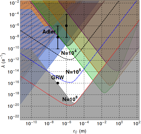
The CSL model contains two new phenomenological parameters: a collapse rate and a resolution length . The differences between standard quantum mechanics and the CSL model depend on the values of these two new parameters. With too small values, CSL predictions are practically indistinguishable from the quantum mechanical ones (the model then looses its effectiveness); on the other extreme, too large values are excluded since then CSL would contradict known experimental facts. Ghirardi, Rimini and Weber proposed a collapse rate s-1 and a resolution length m in their first dynamical reduction model [21], slightly modified later with s-1 (and same resolution length) for the CSL model [15]. Adler proposed stronger values, m and s-1, and m and s-1, based on the analysis of the process of latent image formation in photography [22].
Bounds on the parameters are of course ultimately set by experiments. In the last years, a great effort in comparing collapse models with experiments has been made, through a large variety of experimental setups: from matter-wave interferometry [23], to heating effects in cantilevers [24, 25], to spontaneous X-rays emission from matter [26], which currently sets the strongest upper bound s-1 (for m). The resulting exclusion plot in the parameters space is shown in fig. 2, where the white region must still be experimentally probed, while the non-white regions have been excluded by experiments listed before. Taking into account the challenge to entirely probe this white region by currently used experimental setups, and considering that on-going experiments with atomic gases in double well potentials are able to create and detect strongly correlated entangled states [27], we think is of great interest to study the possibility to perform experimental tests of quantum mechanics using ultracold bosons in Bose Josephson junctions and to determine what requests the experimental values have to satisfy in order to put new bounds on the parameters of the CSL model.
Although the spontaneous localization mechanism of collapse models is very weak, the progresses in the last two decades in the control and manipulation of ultracold gases make such system a promising setup to test the CSL model. Together with their very low temperature ( nK), ultracold atomic systems are characterized by quantum phenomena involving a mesoscopic/large number of atoms ( ranging from to ) [28, 29]. A first work that studied the CSL effects in a cold-atomic system [30] set the upper bound of s-1 (for m) from the analysis of the heating effects on a Bose Einstein condensate. In [31] a theoretical analysis of a recent experiment [32] was performed, where an out-of-equilibrium gas of atoms was cooled to a temperature pK. The dynamical equations for the CSL model were studied, concluding that the resulting bounds are beaten only by measurements of the spontaneous X-ray emission and by experiments with cantilevers. It was as well shown that the bounds are not changed by non-Markovian extensions of the CSL model.
In this paper we study how CSL affects cold atoms in a double well potential, i.e., a Bose Josephson junction, as qualitatively depicted in fig. 1, where we also schematically describe the effect of the collapse of the wave function. A Bose Josephson junction can be experimentally implemented e.g. by superimposing an optical lattice to a parabolic potential [6, 33] or by the use of a laser beam to create the barrier [10]. In a Bose Josephson junction, when the barrier is high enough (much larger than the chemical potential), the atoms can be only in two states. Each wave function is spatially localized in one of the two wells: the higher the barrier separating the two wells, the lower the overlap between the two wave functions. Experimental quantities such as the height of the barrier and the geometry of each well [29], can be tuned with a high degree of control.
A phase difference between the two wells emerges as a consequence of the weak link also for a small number of atoms [34] and it can be fixed (giving rise to the so-called phase state). This possibility for example leads to use Bose Josephson junctions as an atom interferometer [35, 36, 1]. The quantum mechanical evolution of the phase state is characterized by the typical collapse and revival of the interference fringes, while the CSL dynamics decreases the interference until the fringes disappear and each atom is localized in one of the two wells. In this paper we will determine how fast the CSL dynamics collapses phase states, compared to the typical longest coherence time experimentally detected (e.g. ms in [37]).
Besides the phase states, Bose Josephson junctions provide as well a promising possibility for creating macroscopic entangled states, including Schrödinger’s cat states [38, 39]. The use of squeezed states in atomic interferometers and clocks leading to sub-shot-noise performance has been exploited in experiments [13, 14, 40, 41], while the detection of Bell correlations between the spins of atoms in a Bose-Einstein condensate was recently reported in [27]. In this paper, we focus on two types of macroscopic entangled states: the superposition of two phase states and the so-called NOON state. Even if a Schrödinger’s cat state has not been experimentally detected yet in a double well potential, for these two macroscopic entangled states several preparation techniques have been proposed and analyzed [42, 43, 44, 45, 46] (see a review in [47]).
Macroscopic entangled states are of notoriously extremely sensitive to external noise sources. Therefore in this paper we will study the collapse induced by CSL dynamics to the macroscopic entangled states considered here, comparing the result with two typical decoherence sources in optically trapped systems: phase noise [48] and spontaneous photon emission process [49, 50, 51]. The effects of thermal fluctuations and three body recombination terms will be also addressed.
The paper is organized as follows: we start by briefly describing the Bose Josephson junction system within the two mode approximation and introducing the coherent atomic state (or phase state) and the two macroscopically entangled states we consider in our investigation. We then introduce the CSL model, and we find the density matrix evolution for a gas of bosonic atoms in a Bose Josephson junction with CSL dynamics. Next, we find the correlation evolution for the phase state, for the superposition of phase states and for the NOON state. Finally, we compare the CSL dynamics with several typical decoherence sources: phase noise, spontaneous photon emission process, thermal effects and three body recombination terms. A discussion of the results and of perspectives is presented in the conclusions.
II Two-mode model for the Bose Josephson junction
Within the usual two mode approximation [52], valid for large energy barriers between the two wells (and much larger than the chemical potential), one assumes that the atoms can be either in the state of the left well, or in the state of the right well. The left and the right states are taken orthogonal (see [52]). In the second quantization formalism, the Hamiltonian for the interacting gas is
| (1) |
where is the coupling constant of the atom-atom interaction, with the scattering length of the atoms, and we introduced the external double well potential whose specific form determines the left and right Wannier wave functions , (and therefore the coefficients of the two-mode model). The total number of particles is fixed to . Usually, the wave functions , are well approximated from the solutions of the time-independent Gross-Pitaevskii equation:
| (2) |
Denoting by and the ground and the first-excited states of (2), then one has and . This way of constructing the wave functions , is typically good if the number of particles per well is not too large and they do not depend on the interactions via the atom numbers and (in that case one has to resort to a nonlinear tight-binding ansatz [53, 54]).
Let us introduce and the creation (annihilation) operators for, respectively, the left and right states. Rewriting the operators in terms of and as
| (3) |
(with the wave functions , appropriately normalized to ), the Hamiltonian operator in eq. (1) becomes [52, 55]
| (4) |
where and are expressed as appropriate integrals of the wave functions , . In eq. (4) we choose the convention to have positive (negative) for positive (negative), i.e. for repulsive (attractive) interactions. The distance between the wells varies typically between m and m: if the double well potential is created by an optical potential with (being ), then for with m one has that being in the two-mode regime requires kHz [5, 56], while for m is sufficient to have Hz [6]. If the barrier is created by a laser beam having the maximum at the center of the trap, the distance is m in [10] with atoms the barrier was created by a laser beam at 532 nm, blue-detuned with respect to the main optical transition of lithium atoms and at the trap center, the beam was Gaussian-shaped, with a beam waist of m. In this case, in the BEC regime the two-model regime was reached for with the chemical potential , with Hz. In all cases, of course, by increasing the barrier energy the ratio increases (see e.g. [33, 28]; a study of the dependence of the ratio for different dimensionality of the system can be found in [57]). We finally observe that in presence of a negative scattering length, the coefficient can be negative (and yet the two-mode model be valid): the quantum phase transition occurs at a finite value of for which a population imbalance between the two wells has been recently observed [9].
III States
In this section we introduce the states whose collapse (and decoherence) is studied in the following of the paper.
III.1 Phase state
The creation of atomic coherent states using Bose Einstein condensates is a fundamental result for the study of many-body physics with ultracold atoms. Considering our case of interest, the phase state has the following expression [29]:
| (5) |
The phase coherence properties of the above state is expressed by the off-diagonal elements of the single particle density matrix defined as follows
| (6) |
where . Using eq. (5) one has
| (7) |
Coherence properties of the state (5) are detected through the presence of interference fringes in the momentum density of the gas [29]. As discussed in appendix A, the average of the momentum density for a generic state in the symmetric double well potential (4) is
| (8) |
where is the x-component of the momentum . Using eq. (7) for the phase state (5) in the expression (8), we obtain
| (9) |
We observe that the phase coherence (7) is not, generally, a constant of motion of the Hamiltonian (4), due to the presence of the interaction term. In fact, in the case of negligible tunneling, i.e. with , the time evolution of the phase coherence (7) is (see the derivation in appendix B)
| (10) |
where the approximation in the last line holds for small time and large number of atoms (see the study of the phase diffusion in [58, 59]). The phase coherence is periodically reestablished with period [60, 61, 62].
III.2 Superposition of phase states
Bose Josephson junctions are also promising systems to create macroscopically entangled states. The first state considered in this paper is the superposition of phase states as given in (5). They can be dynamically created from a single phase state, with dynamics given by Hamiltonian (4) with . Indeed, after a time , the initial phase state (5) evolves in
| (11) |
where is a fixed phase difference between the two phase states. The state (11) does not show any single-particle coherence properties (7), but it shows -particles coherence. As shown in appendix B one finds
| (12) |
Eq. (12) means that the way to distinguish the state (11) from the statistical mixture is through a measure of -particles observables, i.e., the reduced density matrix at -particles does not show any coherences, except if .
III.3 NOON states
The second macroscopically entangled state considered in this paper is the so-called NOON state, defined as
| (13) |
The NOON state (13) is the ground state of the Hamiltonian (4) with and . Even though several proposals have been formulated to create a NOON state in a double well (see e.g. [42, 43, 44, 45, 46, 63]), its very short life-time with respect to decoherence makes its experimental realization an open problem. A first step in this direction has been done recently [9], where the experimental realization of double well bosonic systems with negative and controllable scattering length was achieved.
A relation similar to eq. (12) is found (see appendix B)
| (14) |
The meaning of eq. (14) is the same as for eq. (12): the only way to distinguish the NOON state (13) from the statistical mixture is by looking at -particles observables.
The fact that NOON state (13) and the superposition of coherent states (5) show similar N-particles coherences can be understood considering that the superposition of coherent states (5) can be obtained from a NOON state passing through a 50:50 beam splitter [38, 44]. The unitary single particle dynamics of the beam splitter does not destroy the initial N-particles coherence of the NOON state. As a consequence, the CSL effects on NOON state and superposition of phase states are the same, as we will see in the next section.
From this point of view, the difference between the atomic coherent state (5) and the macroscopic entangled states (11) and (13) is quite evident. In fact, in the coherent state all the atoms are in the same superposition of single particle states. Single particle observables are enough to detect the quantumness of a coherent state. On the contrary, in the macroscopic entangled states (11) and (13) the superposition is at the level of the whole system and, in order to detect it, the proper -particles observables are required. Notice that differently from the coherence properties (7) of the phase state (5), the -particles coherences (12) and (14) are left unchanged by the Hamiltonian (4) with .
IV CSL model for a Bose Josephson junction
In the CSL model, the density matrix evolution for a bosonic system with particles is described by the following master equation [30]:
| (15) |
where is the number of nucleons in each atom, and and are the parameters characterizing the model, as described in the introductive section.
In order to apply the CSL model to a Bose Josephson junction, it is convenient to rewrite the master equations (15) in terms of the left and right states. Using eq. (3) in eq. (15), we get
| (16) |
where
| (17) |
with . We can immediately note that couplings with an odd number of the same index, like , are null, due to the orthogonality of the two modes. Therefore, we have to evaluate two types of couplings: (i) , where the equality holds because of the parity in the CSL Gaussian term; and (ii) , where the equality holds because of the symmetry of the double well potential.
By taking into account that the total number of particle is fixed, i.e., , it is possible to show that the dissipative term in the master equation (16) takes the following expression:
| (18) |
where we have defined
| (19) |
the last equality is expected to be satisfied in the two-mode approximation.
The master equation (16) then becomes
| (20) |
To have an explicit solution, we neglect the hopping term of (4). As shown in appendix C, the solution of eq. (20) is
| (21) |
where acts on the left (right) of the density matrix, and
| (22) |
is the density matrix evolved under the Schrödinger (unitary) dynamics only.
IV.1 Collapse dynamics due to CSL
Let us see how an initial phase state evolves under the CSL dynamics, looking in particular to the coherence properties given by eq. (7). From eq. (21), it is possible to see that (see appendix C):
| (23) |
Taking into account the Schrödinger evolution of the phase state coherence (10), we obtain
| (24) |
where the last line is valid only for .
From eq. (24), it is clear that the action of the CSL dynamics is to break the spatial superposition (7) of the phase state. Since, in this case, the many-body state is a coherent factorization of delocalized single particle states, then an amplification mechanism is missing, and the CSL collapse rate does not depend on the total number of particles . Thus, the use of phase states such as (5) to set experimental bounds on the CSL parameters is not convenient in general.
As for example, let us consider the experiment [37], where the long coherence time of ms with a gas of 23Na atoms was observed. Using eq. (19), we have that the exponential decrease of the coherence in eq. (24) induced by CSL dynamics becomes experimentally visible only if . Then from eq. (24) it is possible to put a bound of s-1. This is a weak bound for two main reasons: firstly, the expected values of the collapse rate theoretically predicts by Ghirardi, Rimini and Weber ( s-1) and by Adler ( s-1 and s-1) are much smaller than s-1; secondly, much stronger bounds have been set by other experiments, as can be seen in the exclusion plot 2.
Let us now consider the CSL evolution of the macroscopically entangled states (11) and (13). In this case, the -particles coherence properties (12) and (14) are preserved by the Schrödinger evolution. Using eq. (21), as discussed in appendix C it is possible to see that
| (25) |
Differently from the phase decoherence case (24), the exponential decoherence of the macroscopically entangled states (25) is faster due to a factor . This is due to the macroscopicity of the states (11) and (13),i.e., these are superposition of localized -particles states, which is expressed by the -particles quantum coherences (12) and (14). As a consequence, an amplification mechanism occurs in the CSL dynamics, increasing the collapse rate by a factor .
In fig. 2 we show the exclusion plot in the parameters space of CSL [64]. The upper coloured regions indicate the excluded values of the parameters set by experimental data. The lower grey region comes from requiring that the CSL mechanism is strong enough to localize macroscopic objects [23], that is the main motivation that introduced collapse models in first place [16]. Fig. 2 shows also the exclusion plot for an hypothetical experiment involving the macroscopically entangled states (11) or (13). Here, we had to fix a time for which the -particles coherences (12) and (14) are preserved and observed. The longer , the smaller the number of atoms needed to use (the dependence on the time is linear, the one on the number is quadratic). An inspection of results show that in order to have both reasonable values for the particle number and at the same time explore the white region in fig. 2, the one not yet excluded by experiments, one has to use s. This is presently a very challenging request, and the goal of the present computation is to clarify and predict what value of is needed to explore the uncovered region of the CSL parameter space for going from to .
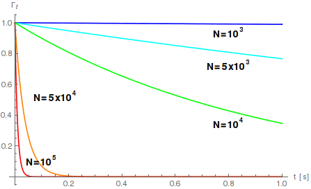
We then choose s and we considered a gas, with width of each well given by , and with the two wells distant . With m is negligible, and the results for apply and are plotted in fig. 2 for three different values of (with m). Also reducing in order to have a finite does not quantitatively change the region that can be explored in the space (actually, we expect it shrinks) - similarly increasing , which results in decreasing , does not change the boundaries of the region, as soon as the two-mode approximation holds. We conclude that with s one needs to enter the white region not yet explored and that with the (presentely prohibitive) number the whole white region can be probed. From fig. (3), where the time evolution (25) is represented, the strong dependence on is clear.
All the computations above have been done under the hypothesis that the unitary Schrödinger dynamics is modified only by CSL noise, without taking into account other decoherence sources. In the next section we compare the main decoherence sources with CSL, and we give estimates on the conditions that experiments must fulfill in order to properly test CSL model.
V Environment decoherence on Bose Josephson junctions and comparison with the CSL model
Problems in testing CSL dynamics in experiments usually arise from environmental decoherence sources, leading to similar loss of coherences. This is the topic of this section, in which we compare the decoherence of the CSL noise with the decoherence induced by the external environment. In particular, we focus on four main sources, i.e., the thermal cloud surrounding the condensate, the three body recombination processes, phase noise and the trapping laser. We then study the conditions that experiments have to fulfil in order to reduce environment decoherence, which is a necessary condition to detect CSL effects. For each decoherence source we consider realistic values of the parameters from typical experimental setups, see e.g. [65, 30, 9]. It turns out that these setups generally present environmental decoherence that covers any CSL effect within the white region of fig. 2. We then estimate what are the values of experimental setup parameters needed to lower environmental decoherence and test CSL according to the analysis described in the previous section.
V.1 Interaction with a thermal cloud
Even if the temperature is very low, a small amount of thermally excited atoms is always present. Atoms in excited states interact with the condensate, leading to two main effects: a loss of atoms from the condensate to the thermal cloud; and a decoherence on the condensate in the position basis. As reviewed in appendix D, the master equation describing the dynamics of a condensate interacting with its thermal cloud is:
| (26) |
where describes the atom losses dynamics, which can be written in the following way for the particular case of a condensate in a double well potential [66]:
| (27) |
where is the rate of atom losses from the condensate to the thermal cloud, which, according the discussion in Appendix D is given by the following local correlation function of the thermal cloud
| (28) |
The term introduced in eq. (26) describes interactions between the condensate (C) and non condensate (NC) atoms of the type . This interaction is in position, and leads to a decoherence dynamics that preserves the populations of the gas. In particular, for a double well potential, the following identity holds
| (29) |
where
| (30) |
Let us consider first the term in eq. (28). Neglecting the Hamiltonian dynamics, it is easy to see that the -particles correlation has the following time dependence:
| (31) |
Differently from the CSL case (25), the decoherence rate induced by atom losses increases linearly with the number of atoms. Therefore, in order to test CSL effects on a NOON state, we need CSL decoherence (25) to be stronger than the decoherence induced by atom losses (31). This means that, if we want to experimentally test CSL in the white region of fig. 2, then we must have , with given by eq. (19). In the particular case of m [15], for typical distances m between the wells (see the discussion in Sec. II).
The one give here above is the general condition to test CSL effects against atom losses. Let us now consider, for example, the experimental setup described in [65], where the authors measured s-1 for a non-homogeneous gas at fractional temperature , whit critical temperature of the gas. Comparing the decay rates of the CSL model in eq. (25) with the decay given by the atomic losses as in eq. (31) with the parameters given in [65], the CSL damping turns out to be faster only if the NOON state is composed by atoms, considering the value s-1 as proposed in [15], and . From eq. (28), the decoherence rate induced by the atomic losses can be reduced either by a proper decreasing of the temperature of the gas (so reducing the thermal density) or by decreasing the coupling interaction, which can be achieved by use of Feshbach resonances. We have that
| (32) |
In order to detect CSL effects on a NOON state with, for example atoms (the number of atoms we need in order to probe the whole unexplored region of the parameter space, as shown in fig. 2), eq. (32) shows that the experimental setup described in [65] must be modified either by reducing the thermal density or by decreasing the coupling constant of one order of magnitude.
Let us now focus on the term in eq. (29). We immediately note the similarities between eq. (29) and the CSL master equation (20), with . Through eqs. (30) and (32), it is possible to relate the decoherence rate due to the atomic losses to the decoherence rate described in eq. (29) as follows:
| (33) |
where is the number of atoms in the thermal cloud. As before, we can experimentally test CSL within the white region of fig. 2 if .
As an example, let us consider again the experiment described in [65], with , where we used the relation between the total number of atoms with the number in the thermal cloud of an ideal gas in an harmonic trap [29]. Using then eq. (33) we have s-1. If and m, then , and s-1. Accordingly, the experimental setup described in [65] must be modified either by reducing the thermal density or by decreasing the coupling constant by two orders of magnitude.
V.2 Decoherence induced by three body recombination processes
We consider in this section the effect of three body recombination processes, according to which atoms leave the trap, with negligible probability that they interact again with other atoms in the trap. We write the effective master equation describing the dynamics of a Bose Einstein condensate with three body recombination processes [67, 68, 66, 69] in the form
| (34) |
where
| (35) |
Using eqs. (34) and (35), one finds the following relation:
| (36) |
where is the condensate density. Comparing the three body decoherence rate in eq. (36) with the CSL decoherence rate , we have a lower bound on the number of atoms of the NOON state:
| (37) |
Consider, for example, the experimental measure described in [65], where and the peak density of the condensate is . In this case, the CSL decoherence is faster if atoms, for the particular case of s-1. The three body decoherence rate can be decreased either by reducing the condensate density or by reducing the scattering length through the use of Feshbach resonance. For example, if we consider an experiment with a condensate density of and a scattering length m, the CSL localization dynamics is dominant with atoms.
V.3 Phase noise
A very common technique to trap atoms is by using an external laser source. Thanks to the large experimental control on the laser electric field, several external potentials can be realized, with a large control on the parameters of the trap [70]. However, every optical trap is also a decoherence source for the trapped atomic system, leading to decoherence of the atomic density matrix in the position basis. Two of the main decoherence sources due to the laser are a phase noise, induced by fluctuations of the laser beam pointing [48], and spontaneous photon emission processes from the atoms [49, 50, 51].
The phase noise in a Bose Josephson junction can be studied and treated as a stochastic noise modifying the energy levels of the system [48]. The effective density matrix evolution is given by:
| (38) |
If the phase noise is a Gaussian noise with null average, then we have that
| (39) |
where the variance completely characterizes the noise. Using eq. (39) in eq. (38), the density matrix evolution of a Bose Josephson junction under a Gaussian phase noise is:
| (40) |
By comparing eq. (40) with the density matrix evolution under the CSL dynamics eq. (21), it is clear that the latter one can be tested only if the phase noise is reduced enough in the experiment. In [30], the authors studied the effect of the fluctuations of the laser beam pointing on a single well potential for a gas of 133Cs atoms. In this work, the heating effect induced by the phase noise turns out to be negligible, compared to the heating of the CSL model, if s-1. If we choose the value m (proposed by Ghirardi et al.l [21, 15]), then, for the experimental setup described in [30], the phase noise becomes negligible if s-1. This means that the interesting part of the parametric space shown in fig. 2 cannot be explored by such experimental setup due to a too strong phase noise. For example, in order to test CSL effects with the parameters s-1 m, then the phase noise should be reduced by a power , showing the very high control on the phase noise needed to explore the parameter space.
V.4 Spontaneous photon emission
Another decoherence source related to optical traps is due to the spontaneous photon emission. In [51], the authors derived the master equation for two levels atoms in a far-detuned optical trap, which is given by:
| (41) |
where is the spontaneous emission rate; , is the frequency of the laser, is the frequency resonance of the two levels atoms; with the speed of light in vacuum; Rabi frequency, related to the effective optical trap by
| (42) |
The function in eq. (41) is defined by the following integration:
| (43) |
We note that the spontaneous emission master equation (41) has the same form as that of the CSL master equation (15), with the replacement:
| (44) |
Using eq. (3) in eq. (41), with a similar procedure used to derive eqs. (16) and (21), it is possible to write down the density matrix for a gas of atoms trapped in an optical trap with spontaneous emission process:
| (45) |
where
| (46) |
Compared to the CSL dynamics given in eq. (21), the spontaneous emission processes are negligible only if . For example, let us consider the experimental setup described in [9], where a laser with wavelength of nm is used to trap a gas of 39K atoms. The resonance frequency of 39K is THz. Setting m, we have that hypothetical CSL effects would be visible only if s-1. This means that the decoherence induced by spontaneous photon emission is strong enough to cover a large part of the parametric space shown in fig. 2. In order to probe the interesting part of the CSL parametric space, the spontaneous photon emission in [9] should be reduced by a power . We conclude that the laser decoherence effects discussed in this and the previous sections are alleviated by using magnetic traps [71]. Thermal and three-body effects cannot be fully removed. Thermal decoherence can be reduced either by weakening the atom-atom interaction, or by lowering the cloud density; three-body effects can be reduced again by weakening the interaction, or by reducing the condensate’s density. This would allow to decrease the number of atom required to test CSL in the white region of fig. 2, from the values discussed in this section to the values presented in Sec. IV.
VI Conclusions
Given the challenge to probe with current experiments the whole white region (not yet explored) in the CSL exclusion plot 2, and motivated by the fact that nowadays experiments with Bose gases in double well potentials are able to create and detect strongly correlated many-body entangled states [27], we studied the possibility to test Continuous Spontaneous Localization (CSL) dynamics in a Bose Josephson junction of ultracold bosons. We also determined what requests the experimental values have to satisfy in order to put new bounds for the parameters of the CSL model in the white region of fig. 2.
The collapse noise localizes the wave function in the position, which means that in a double well there is a localization in the left or in the right states. By solving the CSL exact master equation in the limit of negligible tunneling between the two wells of the potential, we found that the coherence of a phase state is slowly decreased by the localization process of the CSL model. At variance the CSL effects are much stronger in macroscopically entangled states as superposition of phase states and NOON states. Their -atom coherences are suppressed by a factor exponentially depending on the number of atoms, leading to a fast localization process that can be used to test the CSL model. We also compared the CSL dynamics with two typical decoherence sources, namely, the phase noise and the spontaneous photon emission process. Their density matrix evolution mimics the CSL dynamics, and, usually, they are strong enough to cover CSL effects. We discussed under which conditions CSL effects would become stronger than these decoherence sources. We also concluded that magnetically trapped systems are more suitable to test the CSL model. We also compared the results of the CSL dynamics with thermal and three body effects.
Our analysis determines the bounds on the CSL parameters obtainable in experiments with cold atoms. The results are summarized in fig. 2. In the parameter space there is presently a region not yet explored, and we pointed out that having entangled states, as the NOON state, with and coherence time s would make possible to probe such a region. A similar outcome may be obtained when considering entangled states in an array of weakly coupled ultracold bosonic gases described by the Bose-Hubbard model [72] or by varying the distance between (and the width of) the wells.
Although very demanding for current-day experiments, our results together with the recent very promising results on the implementation of squeezed states and the detection multi-particle correlations [27] show that in perspective further advancements in the manipulation of highly-entangled states may open the possibility to study collapse models and to test quantum mechanics with ultracold atoms in double well potentials.
Appendix A Momentum distribution
From a Fourier transform of eq. (3) one finds
| (47) |
For parity symmetry of the double well potential, we can relate the left and right states as follows:
| (48) |
where we imposed that the right well is displaced from the left well along the x-direction.
Appendix B Time-dependent expectation values
From the definition of phase state, using the Hamiltonian (1) with , we have
| (50) |
Considering the superposition of phase states (11) , we have that
| (51) |
With a similar computation, the time evolution of eq. (51) becomes
| (52) |
Appendix C CSL master equation
The general density matrix in the two-mode approximation can be written as follows:
| (53) |
where are complex coefficients satisfying the self-adjointness and normalization conditions of the density matrix. We use the expansion eq. (53) in order to solve the master equation (16), as follows:
| (54) |
From eq. (54), the density matrix is easily obtained.
We also have that
| (55) |
Appendix D Interaction between a condensate and a thermal cloud: master equation and decoherence rates
We derive the master equation describing the dynamics of a Bose-Einstein condensate interacting with its thermal cloud. We start by writing the Hamiltonian of the total system:
| (56) |
We rewrite the Hamiltonian operator in terms of the energy eigenstates of the single particle Hamiltonian :
| (57) |
where
| (58) |
By splitting the condensate modes from the thermal modes , the Hamiltonian operator in eq. (57) becomes:
| (59) |
where
| (60) | ||||
| (61) | ||||
| (62) |
In the interaction picture (labeled by I), an initial density matrix evolves in time as follows:
| (63) |
where refers to time ordering operations. In the weak coupling limit [73], we expand the two time ordered exponentials in eq. (63) up to the second order in the coupling , obtaining the following expression
| (64) |
We work in the Born-Markov approximation [73], with initial state given by
| (65) |
We are interested only in the condensate modes , thus in eq. (64) we perform a partial trace over the non-condensate modes . In computing the reduced master equation for the condensate, we neglect the processes that do not conserve the energy of the system, such as and , where refers to a condensate atom, and refers to a non-condensate atom. We thus obtain the following reduced master equation in the Schrödinger picture:
| (66) |
where
| (67) | ||||
| (68) |
with damping rates given by the following quantities
| (69) | ||||
| (70) | ||||
| (71) |
As one can note, the damping rates introduced in eqs. (70) and (71) are proportional, respectively, to the three-particle correlation and the two-particle correlation of the thermal cloud. For an homogeneous thermal cloud both quantities are strongly peeked around , so we can further simplify the expressions as follows:
| (72) | ||||
| (73) |
where is the Dirac delta. The expressions in eqs. () and () are easily found in standard textbooks on cold atomic systems [74]. Imposing the two-mode approximation on the master equation (66), the eqs. () and () are easily obtained.
Acknowledgements.
Discussions with A. Smerzi are gratefully acknowledged. The authors also thank the anonymous referee for several useful comments. M.B. and A.B. acknowledge financial support from the University of Trieste (FRA 2016). Financial support from INFN is as well acknowledged.References
- [1] A. D. Cronin, J. Schmiedmayer, and D. E. Pritchard, Reviews of Modern Physics 81, 1051 (2009).
- [2] M. Arndt, A. Ekers, W. von Klitzing, and H. Ulbricht, Focus on modern frontiers of matter wave optics and interferometry (New Journal of Physics - IOP Publishing, 2012).
- [3] L. Amico, G. Birkl, M. Boshier, and L.-C. Kwek, Focus on Atomtronics-enabled Quantum Technologies (New Journal of Physics - IOP Publishing, 2015).
- [4] A. Barone and G. Paterno, Physics and applications of the Josephson effect (1982).
- [5] F. Cataliotti, S. Burger, C. Fort, P. Maddaloni, F. Minardi, A. Trombettoni, A. Smerzi, and M. Inguscio, Science 293, 843 (2001).
- [6] M. Albiez, R. Gati, J. Fölling, S. Hunsmann, M. Cristiani, and M. K. Oberthaler, Physical review letters 95, 010402 (2005).
- [7] S. Levy, E. Lahoud, I. Shomroni, and J. Steinhauer, Nature 449, 579 (2007).
- [8] L. LeBlanc, A. Bardon, J. McKeever, M. Extavour, D. Jervis, J. Thywissen, F. Piazza, and A. Smerzi, Physical review letters 106, 025302 (2011).
- [9] A. Trenkwalder, G. Spagnolli, G. Semeghini, S. Coop, M. Landini, P. Castilho, L. Pezzè, G. Modugno, M. Inguscio, A. Smerzi, and M. Fattori, Nature Physics 12, 826 (2016).
- [10] G. Valtolina, A. Burchianti, A. Amico, E. Neri, K. Xhani, J. A. Seman, A. Trombettoni, A. Smerzi, M. Zaccanti, M. Inguscio, et al., Science 350, 1505 (2015).
- [11] A. Smerzi, A. Trombettoni, T. Lopez-Arias, C. Fort, P. Maddaloni, F. Minardi, and M. Inguscio, The European Physical Journal B-Condensed Matter and Complex Systems 31, 457 (2003).
- [12] T. Zibold, E. Nicklas, C. Gross, and M. K. Oberthaler, Physical review letters 105, 204101 (2010).
- [13] C. Gross, T. Zibold, E. Nicklas, J. Esteve, and M. K. Oberthaler, Nature 464, 1165 (2010).
- [14] M. F. Riedel, P. Böhi, Y. Li, T. W. Hänsch, A. Sinatra, and P. Treutlein, Nature 464, 1170 (2010).
- [15] G. C. Ghirardi, P. Pearle, and A. Rimini, Physical Review A 42, 78 (1990).
- [16] A. Bassi and G. Ghirardi, Physics Reports 379, 257 (2003).
- [17] A. Bassi, K. Lochan, S. Satin, T. P. Singh, and H. Ulbricht, Reviews of Modern Physics 85, 471 (2013).
- [18] N. Gisin, Helv. Phys. Acta 62, 363 (1989).
- [19] N. Gisin, Physics Letters A 143, 1 (1990).
- [20] N. Gisin and M. Rigo, Journal of Physics A: Mathematical and General 28, 7375 (1995).
- [21] G. C. Ghirardi, A. Rimini, and T. Weber, Physical Review D 34, 470 (1986).
- [22] S. L. Adler, Journal of Physics A: Mathematical and Theoretical 40, 2935 (2007).
- [23] M. Toroš and A. Bassi, arXiv preprint arXiv:1601.03672 (2016).
- [24] A. Vinante, M. Bahrami, A. Bassi, O. Usenko, G. Wijts, and T. H. Oosterkamp, Phys. Rev. Lett. 116.
- [25] A. Vinante, R. Mezzena, and P. Falferi, arXiv preprint arXiv:1611.09776 (2016).
- [26] C. Curceanu, S. Bartalucci, A. Bassi, M. Bazzi, S. Bertolucci, C. Berucci, A. M. Bragadireanu, M. Cargnelli, A. Clozza, L. De Paolis, et al., Foundations of Physics , 1 (2015).
- [27] R. Schmied, J.-D. Bancal, B. Allard, M. Fadel, V. Scarani, P. Treutlein, and N. Sangouard, Science 352, 441 (2016).
- [28] I. Bloch, J. Dalibard, and W. Zwerger, Reviews of Modern Physics 80, 885 (2008).
- [29] L. Pitaevskii and S. Stringari, Bose-Einstein Condensation and Superfluidity.
- [30] F. Laloë, W. J. Mullin, and P. Pearle, Physical Review A 90, 052119 (2014).
- [31] M. Bilardello, S. Donadi, A. Vinante, and A. Bassi, Physica A: Statistical Mechanics and its Applications 462, 764 (2016).
- [32] T. Kovachy, J. M. Hogan, A. Sugarbaker, S. M. Dickerson, C. A. Donnelly, C. Overstreet, and M. A. Kasevich, Physical review letters 114, 143004 (2015).
- [33] O. Morsch and M. Oberthaler, Reviews of modern physics 78, 179 (2006).
- [34] F. Buccheri and A. Trombettoni, Physical Review B 87, 174506 (2013).
- [35] Y. Shin, M. Saba, T. A. Pasquini, W. Ketterle, D. E. Pritchard, and A. E. Leanhardt, Physical review letters 92, 050405 (2004).
- [36] T. Schumm, S. Hofferberth, L. M. Andersson, S. Wildermuth, S. Groth, I. Bar-Joseph, J. Schmiedmayer, and P. Krüger, Nature Physics 1, 57 (2005).
- [37] G.-B. Jo, Y. Shin, S. Will, T. A. Pasquini, M. Saba, W. Ketterle, D. E. Pritchard, M. Vengalattore, and M. Prentiss, Physical Review Letters 98, 030407 (2007).
- [38] D. Gordon and C. M. Savage, Physical Review A 59, 4623 (1999).
- [39] Y. P. Huang and M. G. Moore, Physical Review A 73, 023606 (2006).
- [40] B. Lücke, M. Scherer, J. Kruse, L. Pezzé, F. Deuretzbacher, P. Hyllus, J. Peise, W. Ertmer, J. Arlt, L. Santos, et al., Science 334, 773 (2011).
- [41] I. Kruse, K. Lange, J. Peise, B. Lücke, L. Pezzè, J. Arlt, W. Ertmer, C. Lisdat, L. Santos, A. Smerzi, et al., Physical Review Letters 117, 143004 (2016).
- [42] J. I. Cirac, M. Lewenstein, K. Mølmer, and P. Zoller, Physical Review A 57, 1208 (1998).
- [43] D. A. R. Dalvit, J. Dziarmaga, and W. H. Zurek, Physical Review A 62, 013607 (2000).
- [44] J. A. Dunningham and K. Burnett, Journal of Modern Optics 48, 1837 (2001).
- [45] P. J. Y. Louis, P. M. R. Brydon, and C. M. Savage, Physical Review A 64, 053613 (2001).
- [46] I. Mazets, G. Kurizki, M. Oberthaler, and J. Schmiedmayer, EPL (Europhysics Letters) 83, 60004 (2008).
- [47] G. Ferrini, Macroscopic quantum coherent phenomena in Bose Josephson junctions, Ph.D. thesis, Citeseer (2012).
- [48] G. Ferrini, D. Spehner, A. Minguzzi, and F. W. J. Hekking, Phys. Rev. A 84.
- [49] C. Cohen-Tannoudji, (1977).
- [50] C. Cohen-Tannoudji, Fundamental systems in quantum optics , 1 (1990).
- [51] H. Pichler, A. J. Daley, and P. Zoller, Physical Review A 82, 063605 (2010).
- [52] A. Smerzi, S. Fantoni, S. Giovanazzi, and S. R. Shenoy, Physical Review Letters 79, 4950 (1997).
- [53] A. Smerzi and A. Trombettoni, Physical Review A 68, 023613 (2003).
- [54] D. Jezek, P. Capuzzi, and H. Cataldo, Physical Review A 87, 053625 (2013).
- [55] J. Javanainen and M. Y. Ivanov, Physical Review A 60, 2351 (1999).
- [56] T. Anker, M. Albiez, R. Gati, S. Hunsmann, B. Eiermann, A. Trombettoni, and M. Oberthaler, Physical review letters 94, 020403 (2005).
- [57] A. Trombettoni, A. Smerzi, and P. Sodano, New Journal of Physics 7, 57 (2005).
- [58] M. Lewenstein and L. You, Physical review letters 77, 3489 (1996).
- [59] J. Javanainen and M. Wilkens, Physical Review Letters 78, 4675 (1997).
- [60] A. Imamoglu, M. Lewenstein, and L. You, Physical review letters 78, 2511 (1997).
- [61] M. Greiner, O. Mandel, T. W. Hänsch, and I. Bloch, Nature 419, 51 (2002).
- [62] D. K. Faust and W. P. Reinhardt, Physical review letters 105, 240404 (2010).
- [63] G. Ferrini, A. Minguzzi, and F. W. J. Hekking, Physical Review A 78, 023606 (2008).
- [64] M. Carlesso, A. Bassi, P. Falferi, and A. Vinante, arXiv preprint arXiv:1606.04581 (2016).
- [65] E. A. Burt, R. W. Ghrist, C. J. Myatt, M. J. Holland, E. A. Cornell, and C. E. Wieman, Physical Review Letters 79, 337 (1997).
- [66] A. Sinatra and Y. Castin, The European Physical Journal D-Atomic, Molecular, Optical and Plasma Physics 4, 247 (1998).
- [67] Y. Kagan, B. Svistunov, and G. Shlyapnikov, JETP Lett 42 (1985).
- [68] P. O. Fedichev, M. W. Reynolds, and G. V. Shlyapnikov, Physical review letters 77, 2921 (1996).
- [69] M. W. Jack, Physical review letters 89, 140402 (2002).
- [70] H. J. Metcalf and P. Straten, Laser cooling and trapping of neutral atoms (Wiley Online Library, 2007).
- [71] J. Fortágh and C. Zimmermann, Rev. Mod. Phys. 79.
- [72] M. Bilardello, Heating effects and localization mechanism in cold Bose gases, Ph.D. thesis, University of Trieste (2016).
- [73] H.-P. Breuer and F. Petruccione, The theory of open quantum systems (Oxford University Press on Demand, 2002).
- [74] C. J. Pethick and H. Smith, Bose-Einstein condensation in dilute gases (Cambridge university press, 2002).