Logarithms and Volumes of Polytopes

In this brief review of projective geometry we follow Ref. [16] and the first appendix of Ref. [17], which provide more complete discussions of these ideas.

A point $\mathbb{Z}^{\alpha}\in\mathbb{CP}^{n}$ is defined by $n+1$ homogenous coordinates, one for each value of $\alpha=0,...,n.$ Each such point defines an $(n-1)$-dimensional hyperplane $H_{Z}$ in the dual $\mathbb{CP}^{n*}$ by placing a single linear constraint on the homogenous coordinates of the dual elements. Namely, we have

The subspace $H_{Z}$ is a linearly embedded $\mathbb{CP}^{n-1}$ in the dual $\mathbb{CP}^{n*}.$ We will refer to linearly embedded $\mathbb{CP}^{1}$’s, $\mathbb{CP}^{2}$’s, and $\mathbb{CP}^{k}$’s with $k>2$ respectively as lines, planes, and hyperplanes, even though the underlying topology of these spaces may be rather different. For example, a $\mathbb{CP}^{1}$ is a Riemann sphere though we will still refer to it as a line.

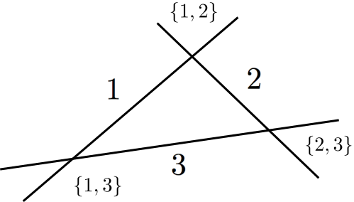
Intersections of lines, planes, and hyperplanes always exist in projective geometry. For example, three points $Z_{1}^{\alpha},$ $Z_{2}^{\alpha},$ and $Z_{3}^{\alpha}$ in $\mathbb{CP}^{2}$ give three lines in the dual $\mathbb{CP}^{2*}$ and each pair of lines intersects in a unique point. This is shown in Figure 1, where the line dual to $Z_{i}^{\alpha}$ is labeled by $i,$ and the intersection of lines $i$ and $j$ is labeled by $\{i,j\}.$

More generally, any two distinct $(n-1)$-dimensional hyperplanes in $\mathbb{CP}^{n*}$ intersect in a unique $(n-2)$-dimensional hyperplane. Namely, two points $Z_{1}^{\alpha}$ and $Z_{2}^{\alpha}$ in $\mathbb{CP}^{n}$ define two $(n-1)$-dimensional hyperplanes $H_{Z_{1}}$ and $H_{Z_{2}}$ in $\mathbb{CP}^{n*},$ and we have that

We therefore see that $n$ distinct points in $\mathbb{CP}^{n}$ uniquely define a point in the dual $\mathbb{CP}^{n*}$ via the simultaneous intersection of their $n$ dual hyperplanes.

There is a natural generalization of the volume of a polytope to projective space. By first understanding this extension for the case of a simplex, the volume of more general polytopes follows immediately by considering sums of simplices. We will therefore follow Ref. [9] and review how to express the volume of simplices in a projective way.

We begin by considering the area of a two-simplex, or a triangle, in real affine space with vertices located at $(x_{1},y_{1}),$ $(x_{2},y_{2}),$ $(x_{3},y_{3}),$ as shown in Figure 2. We can write its area $A$ as [9]

where we have introduced the notation $\langle Z_{1}...Z_{n}\rangle\equiv\varepsilon_{\alpha_{1}...\alpha_{n}}Z_{1}^{\alpha_{1}}...Z_{n}^{\alpha_{n}},$ with the value of $n$ taken from context. We have also defined

as well as

We note that the $Z_{i}^{\alpha},$ $W_{i\alpha},$ and $P^{\alpha}$ all have three homogenous coordinates, in line with their being elements of $\mathbb{CP}^{2}$ (or its dual). We have simply “lifted” the affine coordinates into a particular coordinate patch of projective space by placing a 1 in the third component of the $W_{i\alpha}$’s.

Equation (3) is projectively well-defined in the $Z_{i}^{\alpha}$’s—which, according to the discussion in the previous subsection, determine the faces of the triangle—thus allowing their domain of definition to extend to $\mathbb{CP}^{2}.$ We note that (3) is not projectively well-defined in $P^{\alpha}$ since it defines the line at infinity in $\mathbb{CP}^{2*}$ and therefore the scaling of the area—the scaling we choose here corresponds to the choice of placing 1 (as opposed to a different non-zero number) in the third component of the $W_{i\alpha}$’s. Equation (3) is also completely antisymmetric in the $Z_{i}^{\alpha}$’s, corresponding to the two possible orientations of the triangle.

It will be instructive to see explicitly how this works for one-dimensional simplices as well. A one-simplex is simply a line, and the distance $L$ between two points $x_{1}$ and $x_{2}$ in $\mathbb{R}$ can be written as

Here we have defined

Equation (6) indeed reproduces $L=x_{1}-x_{2},$ as expected, and it expresses the length of the line defined by the endpoints $W_{1\alpha}$ and $W_{2\alpha}$ in terms of their duals and the point at infinity defined by $P^{\alpha}.$ It is projective and antisymmetric in $Z_{1}^{\alpha}$ and $Z_{2}^{\alpha},$ corresponding to the two different orientations of the line.

This generalizes to volumes of simplices in any dimension. For any $D+1$ points $\{Z_{i}^{\alpha}\}_{1\leq i\leq D+1}$ in $\mathbb{CP}^{D}$ there are $D+1$ hyperplanes in the dual $\mathbb{CP}^{D*},$ and the volume of the simplex bounded by these hyperplanes is given by [9]

This expression is projective and totally antisymmetric in the $Z_{i}^{\alpha}$’s. The antisymmetry corresponds to the two possible orientations of the simplex.

The dimension most relevant for scattering amplitudes is four, so for completeness we will explicitly write the volume of a four-simplex, bounded by the five faces defined by $Z_{1}^{\alpha},...,Z_{5}^{\alpha}.$ Translating the above formula gives

For a fixed dimension $D,$ we can view any sum of simplices as the volume of a general polytope, expressed through some particular triangulation. For example, four points $Z_{1}^{\alpha},$ $Z_{2}^{\alpha},$ $Z_{3}^{\alpha},$ and $Z_{4}^{\alpha}$ in $\mathbb{CP}^{2}$ define four lines in the dual $\mathbb{CP}^{2*}.$ These four lines are depicted in Figure 3 and are respectively labeled by 1, 2, 3, and 4.

The area of the shaded quadrilateral can be written as

which is the area of the triangle bounded by the faces 1, 2, and 3 minus the area of the triangle bounded by the faces 1, 2, and 4. This is depicted in Figure 4.

By inspection of Figure 3 we also see that we can write the area of the same region as

by viewing this area as the difference between the area of the triangle bounded by the faces 4, 3, and 1, and the triangle bounded by the faces 4, 3, and 2. We therefore see that we have

which, when one unravels the definition of these 3-brackets, is a non-trivial relation.

Proving this relation through repeated application of Schouten identities on the $\langle...\rangle$ brackets quickly shows that this geometric proof is more convenient, especially for analogous relations in higher dimensions. However, this geometric proof is not very precise, for a few reasons. For one, we have not been careful to keep track of the orientation of the quadrilateral in our two different triangulations. A second and more serious ambiguity is that our notion of a polytope itself is rather tenuous. Namely, once we extend our underlying space from a real affine space to a complex projective space, any notion of “inside” or “outside” is lost. Moreover, one generally thinks of a $D$-dimensional polytope in a $D$-dimensional space as being some full-dimensional region carved out by a finite number of hyperplanes. However, by complexifying our compact space, we end up talking about $D$-dimensional polytopes in $\mathbb{CP}^{D},$ which is a space of $2D$ real dimensions. A third issue with trying to define a polytope as a sum of volumes of simplices is that there are (infinitely) many triangulations that correspond to the same polytope. Some triangulations may make apparent certain geometric qualities of the underlying polytope while masking others.

The amplituhedron makes precise sense of these polytopes as a region in a positive Grassmannian, and for the NMHV case under consideration, this Grassmannian is simply a projective space [5]. In this program one considers convex polytopes, which places positivity constraints on the external kinematics. One then analytically continues to consider general kinematics. In Ref. [12] we instead focused solely on the combinatorial structure of polytopes. We then gave a precise definition of a general type of polytope that is not necessarily convex or even connected. In the next subsection we will briefly review these ideas in two dimensions, as well as introduce the two-dimensional vertex objects $\{F_{ij}\}.$ We refer to Ref. [12] for details and the higher-dimensional cases.

We consider again the quadrilateral in Figure 3 and our goal will be to give it a precise definition. While this figure does not correctly depict the topology of the objects involved—as mentioned above, the lines are actually Riemann spheres—it does correctly depict the intersection structure of these objects. We therefore define this polytope by its intersection structure, saying that this is the “quadrilateral” defined by starting at the vertex $\{1,4\}$ and walking along line 4 to arrive at the vertex $\{2,4\},$ then walking along line 2 to arrive at the vertex $\{2,3\},$ then walking along line 3 to arrive at the vertex $\{3,1\},$ and then walking along line 3 to arrive back at the vertex $\{1,4\}.$ This is depicted in Figure 5.

This set of instructions can be succinctly summarized by the list $(1423),$ which we define to be shorthand for

where each “$\rightarrow$” means to travel along the line whose label is common to the vertex on either side of the arrow.

In Ref. [12] we introduced a collection $\{F_{ij}\}$ of vertex objects defined as a particular sum of volumes of simplices. These objects are referred to as vertex objects because a vertex of a two-dimensional polytope is labeled by two lines, as is each $F_{ij}.$ We found that these vertex objects are antisymmetric, so that $F_{ij}=-F_{ji},$ and that they satisfy¹¹ 1 These vertex objects differ from those introduced in Ref. [12] by a factor of 2.

for any choice of $i,$ $j,$ and $k,$ where we recall that $[ijk]$ is the volume of the two-simplex bounded by the three lines $i,$ $j,$ and $k$.

We consider the sum $F_{14}+F_{42}+F_{23}+F_{31}$ over the vertices of this quadrilateral. Using the antisymmetry of each $F_{ij}$ and equation (14), we find

which is precisely the volume of the quadrilateral that the list of vertices in (13) defines. Applying equation (14) to the left hand side of (15) in a different order also shows that

This gives a quick and rigorous proof of the non-trivial identity (12). Indeed, all possible triangulations of the quadrilateral can be obtained by applying (14) to the left hand side of (15), giving a simple algebraic method for proving many non-trivial identities amongst sums of simplices [12].

This example is a special case of a more general phenomenon—given any set of vertex-connecting instructions defining any polygon, summing the corresponding $F_{ij}$ for each vertex yields the area of that polygon. This process works for general polygons, even disconnected ones. For example, suppose we have six elements $\{Z_{i}^{\alpha}\},$ $1\leq i\leq 6,$ defining six lines, as shown on the left hand side of Figure 6. We can then define the disconnected polygon shown on the right hand side of this figure by the instructions

Analogously to the case of the quadrilateral, this set of instructions corresponds to the list $(51624563).$ It is then the case, rather surprisingly, that the area $A$ of this polygon can be written simply as

This can be checked against any particular triangulation of this polygon. Additionally, any triangulation of this polygon can be obtained from this expression through repeated use of (14).

The general result can be stated as follows. Let $\{Z_{i}^{\alpha}\}$ be a collection of $N$ elements in $\mathbb{CP}^{2}$ defining $N$ lines in the dual $\mathbb{CP}^{2*}.$ The most general polygon in this dual $\mathbb{CP}^{2*}$ is given by a list $(i_{1}i_{2}...i_{n}),$ corresponding to the instructions

The area $A$ of this polygon is then given by the following sum over the vertices:

and from this expression any particular triangulation can be obtained [12]. This form of the area is independent of any particular triangulation and is inherently tied to the data of the polygon itself—its vertices and how we traverse them.

We note that many different lists give rise to the same polygon. For example, any cyclic permutation of a list gives the same polygon. More trivially, the list $(1234)$ is identical to the list $(12121234),$ since the latter corresponds to staying on the vertex $\{1,2\}$ over and over again before moving on. However, the final result in terms of the vertex objects (up to trivial cancellations) is identical. For example, the sum of these objects corresponding to the list $(12121234)$ is simply

which, after using the antisymmetry of $F_{ij}$ yields the same result as the list $(1234).$ Indeed, the sum in (20) is dependent only on the equivalence class of lists, where equivalence of lists is defined by their determining the same polygon. In Ref. [12] we show how to extend this definition of polygon to arbitrary higher-dimensional polytopes.

In Ref. [12] we also defined the corresponding vertex objects in higher dimensions. For example, in three dimensions we defined a collection of vertex objects $\{F_{ijk}\}$ completely antisymmetric in their subscripts and satisfying

for any choice of $i,j,k,l.$ We continue to use the term “vertex objects” because for a three-dimensional polytope a vertex is defined by the intersection of three planes, each defined by a $Z_{i}^{\alpha},$ and these planes determine the subscripts of a given $F_{ijk}.$ In four dimensions we defined a collection $\{F_{ijkl}\}$ of vertex objects that are totally antisymmetric in their subscripts and that satisfy

for any choice of $i,j,k,l,m.$

The volume of any polytope is given by the sum over its vertices of these vertex objects. This expression of the volume is unique, and any triangulation of the polytope can be recovered from this expression using (22), (23), and their higher-dimensional analogues. Additionally, the expression of the volume of a polytope in terms of the vertex objects also encodes the geometry of all lower-dimensional boundary polytopes and readily gives their volumes as well [12].

We note that equation (23) is reminiscent of the formula

given in [9], describing the boundary $\partial[ijklm]$ of the simplex and encoding where the poles of $[ijklm]$ are. Equation (23) does the same, and is also a genuine equality between the volume of the simplex and objects that correspond to its vertices. Thus the objects on the left of equation (23) are fundamentally different than those on the right of equation (24). Similar statements can be made about equations (14) and (22) and the lower-dimensional analogues of equation (24).

Quite surprisingly, the $n$-point NMHV tree-level superamplitude $M_{\rm NMHV}^{n}$ in $\mathcal{N}=4$ planar sYM can be written as the volume of a polytope in $\mathbb{CP}^{4*}$ [9]. Indeed, $M_{\rm NMHV}^{n}$ can be represented as

where the $\{Z_{i}^{\alpha}\}$ implicitly inside the five-brackets in the sum are $n$ points in $\mathbb{CP}^{4}$ encoding the external kinematics and $Z_{*}^{\alpha}$ is a reference vector in $\mathbb{CP}^{4}.$ The sum on $i,j$ is understood modulo $n.$

For any given $n,$ $M_{\rm NMHV}^{n}$ has many different expressions depending on our choice of $Z^{\alpha}_{*}.$ For example, if we choose $Z^{\alpha}_{*}=Z^{\alpha}_{1},$ then for $n=6$ we have

while if we choose $Z^{\alpha}_{*}=Z^{\alpha}_{2},$ then we have

Just as the relation (12) is not obvious at the level of Schouten identities on the $\langle...\rangle$ brackets, the equivalence of the right hand sides of (26) and (27) is non-trivial. These two representations of $M_{\rm NMHV}^{6}$ were initially found by performing two different BCFW shifts on the amplitude [9, 18, 19]. The geometric interpretation is that they correspond to two different triangulations of the same underlying polytope. As discussed in the introduction, their equality can also be understood by using a global residue theorem in an auxiliary Grassmannian [13, 14]. Part of the utility of the vertex objects is to show that the right hand sides of (26) and (27) are equal directly—namely, they are identical when expressed in term of these objects. By using equation (23) on each simplex in either (26) or (27), we find

The amplitude is therefore uniquely expressed in terms of the vertex objects. From this expression and equation (23), any triangulation of $M_{\rm NMHV}^{6}$ can be obtained.

For general $n,$ we have

where in the second equality we used equation (23) and in the last equality we used the cyclicity of the sum and antisymmetry of the vertex objects to cancel in pairs any terms with $*$ as a subscript. This shows manifestly that the amplitude is independent of $Z^{\alpha}_{*}$ and that the underlying polytope has vertices only where the four hyperplanes defined by $Z^{\alpha}_{i},$ $Z^{\alpha}_{i+1},$ $Z^{\alpha}_{j},$ and $Z^{\alpha}_{j+1}$ intersect.

We refer to Ref. [12] for further discussion of this vertex formalism. In the next two sections we show that these vertex objects are naturally defined as contour integrals of logarithms.

As a warmup, we begin our discussion in one dimension. Another way of writing the length $L$ of a line from $x_{1}$ to $x_{2}$ is as

By allowing the $x$ variables to be complex, we can define the complex logarithm function $\log\big(\frac{x-x_{1}}{x-x_{2}}\big)$ with its branch cut connecting the point $x_{1}$ to the point $x_{2}$ along the real axis. We can then rewrite $2\pi i$ as $\text{Disc}\big(\log\big(\frac{x-x_{1}}{x-x_{2}}\big)\big)$—the discontinuity of the logarithm across its branch cut—giving

Unwrapping the contour allows one to drop the “Disc” from the integrand and obtain

where the contour surrounds the cut. Evaluating this explicitly (for example, by going around the pole at infinity) recovers $L=x_{1}-x_{2},$ as expected.

Making the same definitions as in (7) we can rewrite (32) as a contour integral in $\mathbb{CP}^{1*}$ as

where $DX\equiv\varepsilon^{\alpha\beta}X_{\alpha}dX_{\beta}$ is the canonical volume form (of weight two) on $\mathbb{CP}^{1*}$ and $X_{\alpha}\equiv\begin{pmatrix}x\\ 1\end{pmatrix}.$ By explicitly evaluating this integral we find

in agreement with equation (6). In this way, the length of a line is naturally represented as a contour integral of a logarithm.

Motivated by the one-dimensional result, we consider the $\mathbb{CP}^{2*}$ integral

where $DX\equiv\varepsilon^{\alpha\beta\gamma}X_{\alpha}dX_{\beta}dX_{\gamma}$ is the canonical volume form on $\mathbb{CP}^{2*}$ of weight three. The contour is again defined by the integrand in a canonical way: first go around the branch cut of $\log\big(\frac{Z_{3}\cdot X}{Z_{4}\cdot X}\big)$ and then go around the branch cut of $\log\big(\frac{Z_{1}\cdot X}{Z_{2}\cdot X}\big)$. This gives

which is precisely the area of the quadrilateral given in equation (10). If we swap $Z^{\alpha}_{3},$ and $Z^{\alpha}_{4}$ with $Z^{\alpha}_{1}$ and $Z^{\alpha}_{2}$ in equation (35) and pick up a minus sign from the change in orientation of the contour, one readily sees that

thus proving the identity $[123]-[123]=[431]-[432]$ that we obtained in section 2.3. This identity is now made manifest by the integrand of (35).

We have expressed a two-dimensional area as a closed contour integral whose contour specification comes naturally with the integrand itself. The objects whose area we compute in this way are quadrilaterals, defined by four lines. Before describing how the vertex objects are obtained from these kinds of integrals, we quickly discuss how we can use these integrals to compute the volume of three- and $D$-dimensional “quadrilaterals,” or hypercubes.

Consider the following contour integral in $\mathbb{CP}^{3*}:$

where $DX\equiv\varepsilon^{\alpha\beta\gamma\delta}X_{\alpha}dX_{\beta}dX_{\gamma}dX_{\delta}.$ The contour is a three-torus $(S^{1})^{3}$ that goes around the branch cut of each logarithm. We find that

This corresponds to the volume of a three-dimensional “cube,” where we simply mean a polytope bounded by 3 pairs of faces. One way to see that equation (39) is triangulating a “cube” with faces 1 and 2 opposite each other, 3 and 4 opposite each other, and 5 and 6 opposite each other is by examining Figure 7, which shows the superposition of the four simplices in (39) leaving the volume of a “cube.”

As in the two-dimensional case, there is more than one expression for the volume of this cube. Namely, just as we could get two different expressions for the area of a quadrilateral by viewing it as the difference between two different pairs of triangles, we can get three expressions for the volume of the cube as a superposition of four simplices. In particular, we also have

which correspond to the different ways of decomposing the cube analogously to Figure 7 corresponding to Figure 8. Figure 8 is the three-dimensional analog of Figure 4. As in the two-dimensional case, these identities are manifest from the integrand in (38) by swapping, for example, $Z_{1}^{\alpha}$ and $Z_{2}^{\alpha}$ with $Z_{3}^{\alpha}$ and $Z_{4}^{\alpha},$ or with $Z_{5}^{\alpha}$ and $Z_{6}^{\alpha},$ and picking up a minus sign from the change in orientation of the contour.

For completeness we write down the contour integral that gives the volume of a $D$-dimensional “hypercube” bounded by $2D$ faces in “pairs.” With $Z_{1}^{\alpha},...,Z_{2D}^{\alpha}$ defining the $2D$ faces, we have a generalization of the lower-dimensional cases:

where $DX$ is the natural generalization of the lower-dimensional volume forms and the contour goes around the branch cut of each logarithm. We now turn our attention to using these types of objects to obtain the vertex objects and thus to compute the volumes of general polytopes.

Suppose that we have $N$ points $\{Z_{i}^{\alpha}\}_{1\leq i\leq N}$ in $\mathbb{CP}^{2},$ each defining a line in $\mathbb{CP}^{2*}.$ We define the following collection of $\binom{N}{2}$ integrals:

where the contour $\gamma_{ij}$ first goes around all of the branch cuts from $Z_{k}\cdot X=0$ to $Q\cdot X=0$ and then around the branch cut from $Z_{i}\cdot X=0$ to $Z_{j}\cdot X=0.$ The factor of $\frac{1}{2}$ is conventional. Integrating this gives

These are (up to a factor of 2) the vertex objects of Ref. [12] and so in particular we have, for any $i,j,k\in\{1,...,N\},$ that

Each individual vertex object depends on $Q^{\alpha}$ as well as all $N$ of the $Z_{i}^{\alpha}$’s, but the dependence on $Q^{\alpha}$ and all other $Z_{l}^{\alpha}$’s (i.e., for $l\neq i,j,k$) drops out in the above sum.

In equation (46) we wrote $F_{ij}$ as an integral over a function $f_{ij}(X)$ on the dual space. We readily see that $f_{ij}=-f_{ji},$ and can also show that for any choice of $i,$ $j,$ and $k,$

The antisymmetry of the $f_{ij}$’s as well as property (49) imply that the collection of functions $\{f_{ij}\}$ form a representative of a $\check{C}$ech cohomology class on a subspace of $\mathbb{CP}^{2*}.$

In twistor theory, $\check{C}$ech cohomology is a natural setting in which to discuss the Penrose transform, which takes a cohomology class on (a subspace of) twistor space to a finite-normed on-shell field configuration on space-time [16]. The appearance of $\check{C}$ech cohomology here is of a different nature, and the role it is playing in this discussion is still unclear. For the remainder of this note we will not explore this issue. Instead, we simply note this curious connection to cohomology, as it may be important for generalizing these ideas to the N^kMHV amplituhedron with $k>1.$ For now, we simply move on to describing how to construct the higher-dimensional vertex objects in terms of integrals of logarithms.

Analogous vertex objects can be defined in any dimension. Namely, in $D$ dimensions there exist objects $F_{i_{1}...i_{D}}$ such that for any choice of $D+1$ hyperplanes defined by $\{Z_{i_{k}}\}_{1\leq k\leq D+1},$ one has the identity

Given any polytope in $\mathbb{CP}^{D},$ one obtains its volume by summing the vertex objects over the vertices of the polytope. In particular, any vertex of the polytope is defined (as reviewed in section 2) by the intersection of $D$ hyperplanes corresponding to $Z_{i_{1}},...,Z_{i_{D}},$ and for this vertex one simply includes an $F_{i_{1}...i_{D}}.$ The precise definition of higher-dimensional polytopes in $\mathbb{CP}^{D}$ is described in Ref. [12], as is the precise way of summing the vertex objects over the vertices. In this subsection, we will see how these higher-dimensional vertex objects arise as contour integrals of logarithms. We will explicitly show this only for dimensions three and four.