Magnetic order in 4-layered Aurivillus phases
Abstract
We determine the viability of 4-layered Aurivillius phases to exhibit long-range magnetic order above room temperature. We use Monte Carlo simulations to calculate transition temperatures for an effective Heisenberg model containing a minimal set of required couplings. The magnitude of the corresponding coupling constants has been determined previously from electronic structure calculations for , for which we obtain a transition temperature far below room temperature. We analyze the role of further neighbor interactions within our Heisenberg model, in particular that of the second-nearest-neighbor coupling within the perovskite-like layers of the Aurivillius structure, as well as that of the weak inter-layer coupling, in order to identify the main bottleneck for achieving higher magnetic transition temperatures. Based on our findings, we show that the most promising strategy to obtain magnetic order at higher temperatures is to increase the concentration of magnetic cations within the perovskite-like layers, and we propose candidate compounds where magnetic order could be achieved above room temperature.
I Introduction
Coexistence of ferroelectricity and magnetic long-range order in the same material is an uncommon phenomenon [1]. Materials that exhibit such coexistence are called magnetoelectric multiferroics [2]. In recent years, such materials have attracted huge interest,[3, 4] motivated in large parts by the possibility of exploiting the coexistence of the two types of long-range order to create four-state logic devices,[5] and by the prospect of using cross-couplings to switch magnetic bits with an applied voltage.[6] Two main routes that can lead to magnetoelectric multiferroic states are often distinguished [7]. The first one requires the presence of particular types of magnetic order that break inversion symmetry (e.g. spiral states in MnO3 [8]) and hence can couple to electric polarization. The second route is realized in compounds in which ferroelectricity is induced by a structural instability that is only weakly affected by magnetic order. A prominent example for this second scenario is BiFeO3, which is one of the most extensively studied multiferroics.[9] Due to the relative scarcity of magnetoelectric multiferroics, the design of new materials with robust multiferroic properties above room temperature is very desirable.
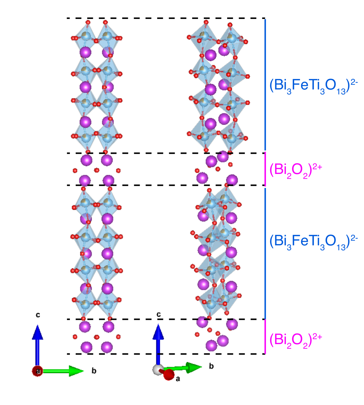
The Aurivillius phases are a family of naturally-layered oxides. Their structure consists of perovskite units, (O3m+1)2-, stacked along the direction, and alternating with fluorite-like layers of (Bi2O2)2+ (see Fig. 1 for a case with ). [10] Aurivillius phases are well known for their good ferroelectric properties with Curie temperatures well above room temperature and low fatigue[11, 12]. Furthermore, Aurivillius phases display a large chemical flexibility, which allows to incorporate various magnetic (and non-magnetic) cations on the octahedrally coordinated sites, making this class of materials a very promising starting point for engineering high temperature multiferroics. In particular, Aurivillius systems incorporating transition metal cations, which generally can give rise to high Néel temperatures in oxides, are natural candidates to explore new multiferroic compounds.
Experimentally, most efforts so far have focused on structures with 75 % and 25 % (or other magnetic cations with valence ) distributed over the sites.[13, 14, 15, 16] However, conflicting magnetic properties have been reported for these compounds. In the most studied case of , Srinivas et al. have reported an antiferromagnetic transition temperature of 80 K[17], which conflicts with more recent studies that report paramagnetic behavior with no magnetic long-range order down to very low temperatures.[13, 18, 19] Furthermore, it was shown that the observed properties often depend strongly on the synthesis conditions and can be caused by trace amounts of impurity phases, which are very hard to detect using standard laboratory-based characterization methods [20]. Therefore, it is of great interest to have a theoretical estimation of the expected magnitude of the temperature, , at which magnetic order might arise.
From the theoretical side, two factors appear crucial for the possible emergence of long-range magnetic order in Aurivillius phases. The first is the relatively low concentration of magnetic cations (only 25 % on the perovskite sites in the above examples), the second is the short range of the superexchange interaction, which is the dominant coupling mechanism between magnetic ions in insulating oxides.
The concentration of magnetic cations is fixed by stoichiometric constraints. As already mentioned, most systems that have been studied so far correspond to 4-layered () Aurivillius phases with composition BiTi3O15, where is a trivalent transition metal cation. Note that due to the different valence it is not possible to simply substitute some of the Ti4+ by to increase the concentration of magnetic cations on the sites. In Sec. III.3 we discuss possible alternative compositions that allow to increase the concentration of magnetic cations, but first we will focus on already existing compounds with and 25 % magnetic cations on the -sites, in particular the case with =.
For this relatively low concentration of magnetic ions, the short range of the superexchange mechanism represents a serious challenge for obtaining long-range magnetic order at high temperature. Typically, superexchange can be very strong between magnetic ions sharing the same ligand (i.e. nearest-neighbor superexchange), but decreases quickly with distance (or, more precisely, with the number of bonds along the shortest superexchange path connecting two magnetic ions).
The low concentration of magnetic ions (25 % in the above examples) results in a low average number of magnetic ions that share an oxygen ligand and thus are strongly coupled. In the worst case, the percolation threshold for a fully connected network of nearest-neighbor superexchange bonds might not be reached, and the system simply consists of many isolated clusters that are only weakly coupled by further-neighbor superexchange interactions. However, even somewhat above this percolation threshold, the effective dimensionality of the resulting “magnetic lattice” can be quite low. This implies that the much weaker further-neighbor superexchange couplings are playing a crucial role for achieving long-range order in and similar Aurivillius phases. In particular, due to the presence of the (Bi2O2)2+ layers (see Fig. 1), there are no strong nearest-neighbor links between adjacent perovskite blocks, which are only coupled through rather weak further neighbor superexchange (the shortest possible superexchange path between two adjacent perovskite blocks is along a sequence of -O-O-O- bonds). However, coupling across the ()2+ layers is essential to achieve long-range order along the direction, and its small size might critically affect the transition temperature.
For the case of , magnetic coupling constants have been calculated using first principles electronic structure calculations. [21] Indeed, a rather strong coupling for cations in nearest-neighbor positions of around 45 meV, corresponding to a temperature scale of 520 K has been obtained. In contrast, the coupling between cations in next-nearest-neighbor positions is more than one order of magnitude smaller (1-2 meV, corresponding to 15 K), and the inter-layer coupling was estimated to be around 0.3 meV ( 3.5 K).
In this article, we present Monte Carlo simulations for an effective Heisenberg model applicable to Aurivillius systems. Based on the coupling strengths calculated for , we obtain an upper bound for the magnetic transition temperature () of this material of 22 K, i.e. significantly below room temperature. In order to explore which of the two weak further-neighbor couplings represents the more severe bottleneck for obtaining high , we individually vary the strength of the next-nearest-neighbor coupling within the perovskite blocks as well as that of the inter-layer coupling. These calculations show that, for a magnetic ion concentration of 25 %, the next-nearest-neighbor interaction is crucial to achieve good percolation (and thus high ) within the perovskite blocks, but that the influence of the weak inter-layer coupling is less severe. We then also vary the concentration of magnetic ions on the sites of the model, using realistic magnitudes for the coupling constants based on the calculated values for . We show that high transition temperatures can in principle be achieved for concentrations above 50 %, in spite of the rather weak inter-layer coupling. Finally, we propose a route to achieve such higher concentrations of magnetic ions by substituting with non-magnetic cations with higher valence, such as Nb5+, Ta5+, Mo6+, or W6+.
The paper is structured as follows. In Sec. II we first describe our model, discuss its limitations, and clarify which couplings beyond nearest-neighbor we consider. In the same section we also specify the technical details of our simulations. In Sec. III.1 we then present and discuss the results obtained for and investigate the dependence of on the strength of further-neighbor couplings within and in between the -perovskite blocks. In Sec. III.3 we discuss the dependence of the transition temperature on the concentration of magnetic ions, and we propose possible compositions with concentrations larger than 25 %. Finally, in Sec. IV we summarize our main conclusions.
II Model and Methods
II.1 Model and Couplings in 4-Layered Aurivillius Phases
In this section we discuss the effective model that we use for a generic value of magnetic ion concentration, , on the sites of an Aurivillius phase. As the network of superexchange bonds is determined by the specific distribution of magnetic and non-magnetic cations over the available sites, we first discuss the method by which we distribute the magnetic ions within our simulation cell. Then, we describe the relevant magnetic couplings that we consider, and finally we define the specific Heisenberg Hamiltonian that we use in our simulations.
The conventional (primitive orthorhombic) unit cell of the ferroelectric structure of and related 4-layered Aurivillius phases with space group symmetry consists of four formula units (f.u.). However, for our model we need to consider only the sites that can potentially be occupied by magnetic cations, and thus the cell we use in our simulations is based on the simple tetragonal cell sketched on the left in Fig. 2. This cell contains two f.u., or sites, stacked along the direction. The lateral shift between subsequent groups of 4 sites is related to the -layer in between two 4-perovskite blocks.
We then construct an supercell of the basic cell. This supercell contains sites, over which we have to distribute a total of magnetic cations. In order to avoid creating configurations with an extremely inhomogeneous distribution of magnetic cations, we first divide the full supercell into intermediate cells (see middle part of Fig. 2), and then randomly distribute the magnetic cations with the constraint that stoichiometry is satisfied within each intermediate cell. Thus, the resulting concentration of magnetic sites is exactly equal to within each intermediate cell. We note that configurations where stoichiometry would be violated over larger volumes will be strongly disfavored in the real material due to the Coulomb interaction. We use a size of in units of the basic cell for these intermediate cells.
Note that we use a supercell with 8 times more basic unit cells along the two in-plane directions than along the direction, in order to obtain an aspect ratio of the final simulation cell close to one (in terms of number of adjacent sites). This is also expected to reduce the temperature range for which the correlation length becomes comparable with the system size. Due to the rather weak inter-layer coupling between the -perovskite layers, the correlation length is expected to be smaller along the direction than along the perpendicular in-plane directions.
We point out that, apart form the stoichiometry constraint on the intermediate cell level, we use a completely random (homogeneous) distribution of magnetic cations over the available sites. Even though Ref. 21 reported a preference of to occupy the inner site in , this tendency is not very strong. Furthermore, a homogeneous random distribution of magnetic ions is presumably most favorable for the development of long-range magnetic order, and since we primarily want to establish an upper bound for the magnetic transition temperature, we are focusing here on this most favorable case. Furthermore, we make no assumptions on potential correlations between the relative positions of magnetic ions on neighboring sites.
Once a specific distribution of magnetic ions on the sites is constructed, it is possible to establish the network of exchange couplings connecting the magnetic sites. As discussed in Ref. 21, one can in principle distinguish four different, symmetry-inequivalent couplings between magnetic ions in “nearest-neighbor” positions within the perovskite blocks. However, ab-initio calculations for presented in Ref. 21 also show that at least three of these nearest-neighbor couplings have very similar strength. For simplicity, and since our main goal is to establish an upper bound for the magnetic transition temperature, we consider all nearest-neighbor couplings to be identical for the purpose of this work, and we denote the corresponding coupling strength by .
Now, considering only the network of spins connected by , each of the 4-perovskite blocks is effectively a simple cubic lattice with only four layers along . Each site of this lattice is then randomly occupied with probability . The problem of finding the minimal average occupation of sites, , necessary to obtain site percolation through nearest-neighbor bonds in a simple cubic lattice has been studied extensively, [22, 23, 24, 25, 26] and the critical concentration was found to be . This implies that for the case of the 4-layered Aurivillius phases with composition BiTi3O15, i.e. , no magnetic long-range order can be obtained by considering only , and thus further-neighbor couplings play an essential role for the magnetic ordering. Therefore, we also include magnetic coupling between next-nearest-neighbor positions within the -perovskite blocks into our model. The values of some of these couplings for the case of have also been calculated in Ref. 21 and, similar to the nearest-neighbor couplings, can be viewed as approximately constant and independent of the specific next-nearest-neighbor configuration. Thus, we use the same coupling constant, , for all next-nearest-neighbor bonds within the -perovskite blocks of our model.
Although the presence of such a next-nearest-neighbor coupling guarantees to overcome the percolation threshold within the -perovskite blocks for a concentration of ( for a simple cubic lattice with both nearest and next-nearest neighbor couplings [26]), so far our model does not include any coupling between adjacent -perovskite blocks. Therefore, to achieve three-dimensional long-range magnetic order it is essential to also consider a coupling between closest neighbors across a -layer, i.e., between two adjacent -perovskite blocks. We denote this inter-layer coupling by .

Thus, the minimal model necessary to describe long-range magnetic order in 4-layered Aurivillius phases with a concentration of magnetic cations on the sites must involve at least the following three couplings: , , and . Other further-neighbour couplings are either weaker, or are not relevant for achieving long-range order, and are therefore neglected within our model. The three types of coupling that we consider in our model are illustrated in Fig. 3.
The Hamiltonian of the system is then expressed in the standard Heisenberg form:
| (1) |
where is a three-dimensional unit-length vector describing the direction of the magnetic moment at site , and the summation is over all sites occupied by magnetic ions. Here, can have the values , , or , depending on whether and are, respectively, nearest-neighbors, next-nearest-neighbors within the -perovskite blocks, or closest possible neighbors across a -layer. In all the other cases, is zero. We also consider a small easy axis anisotropy, , in Eq. (1), in order to have a well-defined order parameter along the direction.
Unless stated otherwise, the strengths of the three coupling constants used in our simulations are set to values corresponding to those obtained from ab-initio calculations for in Ref. 21: meV, meV, and meV. Furthermore, we set meV. Note that all quantities in Eq. (1) are defined considering as a unit vector, while the size of the magnetic moments is absorbed in the coupling constants and in .
We note that the coupling constants obtained in Ref. 21 are all antiferromagnetic, i.e., corresponding to a negative sign of in Eq. (1). This can result in closed loops of bonds that are partially frustrated, e.g. bonds relative to the couplings and as shown for the bonds marked by the red circle in Fig. 3. In order to avoid complications in the Monte Carlo simulations due to such partial frustration, and since we mostly want to provide an upper limit for the transition temperature, we neglect the possible role of frustration in decreasing by assuming all couplings to be ferromagnetic, i.e. with positive sign.
II.2 Monte Carlo Simulations
To obtain temperature dependent properties for the model described in the previous subsection, we perform Monte Carlo simulations using the Metropolis algorithm and parallel tempering. [27] Furthermore, we average the so-obtained macroscopic quantities over several realizations of the magnetic cation distribution. In practice, we apply the following procedure:
- 1.
Generate a random distribution of magnetic cations within our simulation cell (respecting the constraint discussed in the previous section).
- 2.
Determine the network of bonds for each type of coupling.
- 3.
Use Monte Carlo to calculate thermodynamic quantities for this specific configuration.
- 4.
Repeat this procedure several times, each time generating a different random distribution of magnetic cations over the site positions.
- 5.
Take the average of the quantities obtained for each specific cation distribution.
Furthermore, we repeat this procedure for different system sizes to obtain an accurate estimate of in the limit of infinite system size. For this purpose we note that, due to the small easy-axis anisotropy included into the model, the relevant order parameter is , the component of the magnetization along the easy axis. Here, indicates an average over Monte Carlo measurements, while indicates the average over different configurations, i.e., different realizations of the magnetic cation distribution. We average over different cation distributions to account for the self-averaging present in macroscopically large samples.
Thus, can be determined from the crossing point of Binder cumulants [28, 29] of calculated for different system sizes,[30] where the Binder cumulant is given by:
| (2) |
Furthermore, we also calculate the magnetic susceptibility:
| (3) |
where is the temperature and is the Boltzmann constant.
Typically, temperatures are run in parallel using the parallel tempering procedure. Temperatures are distributed exponentially according to , where and . We use the same values for and for all simulations with the same , independent of the size of the system. Measurements of magnetization and energy are collected every sweeps (average number of update trials per spin). A certain number of initial measurements (typically ) are not included in the averages for thermalization purposes, and averages are taken over a number of measurements varying between and , depending on system size.
III Results and Discussion
III.1 Transition temperature for
We begin the discussion of our results by considering the case of , i.e. a concentration of and all coupling constants fixed to the approximate values calculated in Ref. 21, as specified in Sec. II.1. Fig. 4 shows the temperature dependence of the magnetization, magnetic susceptibilities, and Binder cumulants for different sizes of the simulation cell. In each case, all quantities are obtained by averaging over an ensemble of 5 configuration corresponding to different distributions of the cations.
From the crossing point of the Binder cumulants for the three different system sizes, we obtain a magnetic transition temperature K. This value is also consistent with the temperature dependence of the magnetization and with the peak positions of the magnetic susceptibility, which appear to depend only weakly on system size.
The value of K is more than two orders of magnitude smaller than . This small value of the transition temperature arises from the fact that the concentration of Fe3+ in is too low to allow percolation of the nearest-neighbor bonds within the -perovskite blocks (see the discussion in the previous section). Therefore, the system essentially consists of small isolated clusters of , where the magnetic moments within each cluster are coupled strongly through , but different clusters within the same -perovskite block are only weakly coupled through . Furthermore, different 4-perovskite blocks are coupled through the very weak interaction .
This low value of , which, based on the nature of our approximations, can be viewed as an upper limit to the magnetic transition temperature of the real material, indicates that claims of room-temperature magnetism measured in are very unlikely related to the intrinsic properties of this material. Instead, inclusions and other magnetic impurities are most likely responsible for the apparent high temperature magnetic properties. We also note that the superexchange interaction between cations is generally one of the strongest among all transition metal cations, and thus the same conclusion holds for similar reports on related 4-layered Aurivillius phases containing other transition metal cations with concentration .
In the following, we establish the sensitivity of the calculated on the specific values used for and . This also allows to identify which coupling constitutes the more severe bottleneck for achieving higher transition temperatures and thus should possibly be increased, e.g. by applying strain or pressure, to best engineer 4-layered Aurivillius phases with magnetic order at higher temperatures.
III.2 Dependence of on and
Next, we investigate the dependence of the transition temperature on the weak further-neighbor couplings and . To this end, we perform analogous simulations as described on the previous section, but with varying strength for one of these coupling constants, while the other one is set to be equal to . In this way, there is always only one “weak” coupling in the system, and one can observe how is reduced on decreasing the strength of this particular coupling constant. These calculations are performed for a system containing basic unit cells, and concentration of magnetic ions fixed to . Since the purpose of these calculations is not to obtain an extremely accurate value for , but rather to observe the trend as the coupling constants are tuned, we do not obtain the transition temperature using the intersection of Binder cumulants for different system sizes. Instead, we extract the peak position of the magnetic susceptibility for eight different random distributions of the magnetic ions. We then estimate the transition temperature by averaging this peak position over all eight configurations, and we estimate the corresponding error using the standard deviation of the different values.
We first consider the case where all couplings have the same size as , i.e. meV. It can be seen from Fig. 5 that, although the overall energy scale of the couplings is quite large (520 K), we obtain a transition temperature K, which is only slightly above room temperature. This is due to the low concentration of magnetic ions, resulting in a low average coordination number of the magnetic lattice.
Keeping meV, we then decrease in several steps from 45 meV to 0.45 meV. The resulting transition temperatures are shown as black dots in Fig. 5. Interestingly, the transition temperature exhibits only a moderate decrease (by approximately a factor 0.5) although is decreased by two orders of magnitude.
Next, we keep meV and decrease the value of stepwise from 45 meV to 0.45 meV. The resulting transition temperatures are indicated as red squares in Fig. 5. We observe that, in this case, the value of decreases more dramatically compared to the previous case where is decreased.
The reason for this profound difference regarding the sensitivity of on compared to can be qualitatively explained as follows. For , the system consists of uncoupled 4-layers, while the network of bonds created by and percolate each individual 4-layer. Thus, the system essentially represents a quasi-two-dimensional system (see Refs. 31, 32). In this case, and considering isotropic spins (i.e., neglecting the small easy axis anisotropy in the model), the correlation length perpendicular to would diverge as . Thus, when is switched on, the effective net interaction between the 4-layers, and thus the energy-scale determining the temperature for long-range magnetic ordering, is not simply given by . Instead, it is given by multiplied by the number of correlated spins within each layer, i.e. all spins within a radius of the size of the correlation length at that temperature. This implies that the transition temperature has a relatively weak dependence on the inter-layer coupling.
A similar scenario does not occur, however, in the limit of small . In this case, the bonds created by and are not sufficient to overcome the percolation threshold within the system, both within the 4-layers and along . Thus, for , the system consists of a conglomeration of uncoupled clusters, and the correlation length is limited by the average size of these clusters. For and temperatures at which the correlation length is of the size of each cluster, the system resembles isolated magnetic moments of different sizes (corresponding to the cluster sizes) coupled by . This would imply a linear dependence of on . However, since the concentration of is relatively close to , the typical size of the clusters might be relatively large and thus the temperature at which all spins within the clusters are fully correlated might be quite small.
This scenario is qualitatively supported by the behavior of the magnetic susceptibility above , calculated for different values of and . Within this paramagnetic regime, the susceptibility is expected to exhibit Curie-Weiss behavior, i.e., , where the constant is proportional to the square of the effective magnetic moments. Thus, if interactions occur between clusters of correlated spins, one expects to be quite large. We can extract by taking the inverse of the numerical derivative of , i.e. . Fig. 6 shows the so-obtained values for temperatures above and for the various values of and . It can be seen that one obtains rather large “effective moments” when is decreased, even at temperatures around 200 K. In contrast, the effective moments remain small down to rather low temperatures on decreasing . This indicates that, at a given temperature, the size of the correlated clusters of spins is much larger when the system resembles weakly coupled two dimensional layers, than when the system resembles weakly coupled non-percolating clusters.
We point out that the realistic values for and ( meV and meV, respectively) are both very low compared to the strong nearest-neighbor coupling ( meV) in . Therefore, the real system corresponds to weakly coupled layers formed by weakly coupled clusters, which explains the low transition temperature found in Sec.III.1. Furthermore, this suggests that a large enhancement of and in particular of would be necessary to increase the transition temperature towards higher values. While it is in principle conceivable to enhance and via pressure, strain, doping, or cation substitution, it appears quite unlikely that the required order-of-magnitude changes can be achieved in this way. Therefore, the most promising route to obtain Aurivillius phases with magnetic long-range order at or above room temperature is to increase the concentration of magnetic ions.
III.3 Aurivillius phases with higher concentration of magnetic cations
Motivated by the results presented in the previous sections, we now consider also magnetic ion concentrations larger than 25 %. Generally, the achievable concentration of magnetic cations in Aurivillius phases is constrained by stoichiometry and size restrictions. Only cations within a certain size range have been found suitable to occupy the sites within the Aurivillius structure[10]. Most magnetic cations that are within this suitable range have a valence of , e.g. Fe3+, Co3+, Cr3+, or Mn3+. However, a total of electronic charges have to be balanced by the cations occupying the sites and the sites. Typical site cations in the Aurivillius phases have either a valence of or , with Bi3+ perhaps being most common. Thus, with Bi3+ (or any other possible cation) on the site, the required average site valence is given by . This implies that it is not possible to have all available sites occupied with magnetic cations (except in the limit ). Instead, a certain percentage of sites has to be occupied by nonmagnetic cations with higher valence, such as e.g. as in . Note that it has been found impossible to incorporate significant amounts of the higher-valent (and rather small) Mn4+ cation into the Aurivillius structure [33, 34].
Based on these restrictions, there are in principle two ways to increase the concentration of magnetic cations. The first possibility is to increase , the number of layers within the perovskite blocks, which decreases the required average site valence . Indeed, magnetic long-range order has been reported for several systems.[19, 35] The second possibility, which we explore in the remainder of this article, is to keep fixed and substitute with nonmagnetic cations of even higher valence, such as Nb5+, Ta5+, Mo6+, or W6+. For this leads to compositions such as e.g. Bi5Fe1+xTi3-2xNbxO15 or Bi5Fe1+2xTi3-3xWxO15 (). In Table 1, we propose some examples for Aurivillius phases that correspond to higher magnetic cation concentration and higher critical temperatures. While (with ’s exception and to the best of our knowledge) none of these compounds have been synthesized yet, the suggested cations have all been successfully incorporated on the sites of other known Aurivillius phases.
| estimated (K) | 22 | 204 | 455 | 701 |
|---|---|---|---|---|
| concentration (%) | 25 | 50 | 75 | 100 |
| example Aurivillius | ? |
In the following we assume that increasing the number of (or other magnetic cations) and replacing part of the with higher-valent non-magnetic cations will not significantly alter the magnitude of the three relevant magnetic coupling constants considered in our model. We thus keep the values for , and fixed to the ones derived from the ab-initio calculations for . [21] The most relevant effect resulting from the increased magnetic ion concentration that is included in our model is therefore the increasing amount of bonds between magnetic ions coupled through the strong nearest-neighbor coupling .
We consider the concentrations , , and , and perform Monte Carlo simulations for supercells of sizes , , and in units of the basic cell. Similar to what was discussed in Sec. III.1, the macroscopic averages obtained for and are averaged over five different random distributions of magnetic cations.
Fig. 7 shows the temperature dependence of the magnetic susceptibilities (upper panels) and Binder cumulants (lower panels) for the three concentrations of magnetic ions on the sites. For all three concentrations, the Binder cumulants obtained for differently sized simulation cells intersect at a temperature very close to the peak position of the magnetic susceptibility calculated for the largest system size. This indicates that finite size effects are relatively small in this case. Furthermore, the transition temperature for , i.e., when half of all sites are occupied by magnetic ions, is significantly higher than for , but still below room temperature. However, for , long-range magnetic order appears at temperatures well above 100∘C. Finally, when all sites are occupied by magnetic ions, i.e., for , we obtain K.
The transition temperatures obtained for different concentrations are summarized in Fig. 8. Since the energy scale (and thus the specific value of ) in the Monte Carlo simulations is defined via , we also include scaled values of , which correspond to different strength of (but fixed ratios and ), e.g. for magnetic cations other than . We note that, for concentrations above the critical value for percolation of the nearest-neighbor bonds (), the transition temperature seems to increase linearly with concentration.
Measurements of magnetic properties on Aurivillius phases Bim+1Ti3Fem-3O3m+3 performed by Jartych et al. [19] indicate transition temperatures to a spin glass state of K and K for and ( and ), respectively. These values are quite comparable in size to the transition temperature we obtain for (see Fig. 8 and Table 1). Furthermore, the value of K obtained for is rather similar to the Néel temperature of the perovskite BiFeO3 ( K) [36].
Even though this comparison should be taken with care, since the values obtained from our simulations should merely be interpreted as upper bounds for the transition temperatures of the real materials (with partially frustrated antiferromagnetic interactions), this seems to indicate the following: 1) the magnitudes we used for and the assumption that depends only weakly on concentration are indeed reasonable, 2) the weak inter-layer coupling is not prohibitive for achieving transition temperatures around or above room temperature, and 3) the partial frustration of antiferromagnetic bonds is not very strong, at least for cases with .
IV Summary and Conclusion
In this work, we have, from a theoretical perspective, explored whether Aurivillius phases can exhibit magnetoelectric multiferroic states at or above room temperature. To this end, we have established a Heisenberg model corresponding to magnetically-dilute 4-layered ferroelectric Aurivillius phases. The minimal model for which magnetic long-range order can occur within these compounds, including the important case with only 25 % of all sites occupied by magnetic cations, requires the presence of nearest-neighbor, next-nearest-neighbor, and inter-layer couplings. To obtain the corresponding magnetic transition temperatures, we have performed Monte Carlo simulations, thereby averaging over several distributions of magnetic cations over the available sites. We obtain upper limits for the transition temperature by neglecting the partial frustration that can occur in the case of antiferromagnetically coupled spins.
For the case of (concentration ) we use coupling constants based on earlier ab-initio calculations, and we obtain a transition temperature of K, i.e. far below room temperature. In order to identify the most promising strategy for achieving magnetic long-range order at higher temperatures, we have then addressed the individual effects of the weak next-nearest-neighbor coupling within the 4-perovskite blocks, , and of the weak inter-layer coupling between these blocks, . Our results indicate that the most crucial coupling in the dilute () case is . Even though the presence of the inter-layer coupling is crucial to achieve percolation along the direction, the strength of has a much stronger impact on the transition temperature. A significant increase of with respect to the value obtained from ab-initio calculations for seems necessary to achieve magnetic order around room temperature. However, it is unclear whether and how such a significant increase of could be realized.
Therefore, we have explored a more promising route toward higher , which is to increase the concentration of magnetic ions within the -perovskite blocks. For the case considered here, our results indicate that for , magnetic transition temperatures around or above room temperature can be reached. To obtain 4-layered Aurivillius phases with increased magnetic ion concentrations, we suggest to combine trivalent magnetic transition metal cations such as with high-valent non-magnetic cations such as e.g. Nb5+, Ta5+, Mo6+, or W6+. The calculated transition temperatures as well as some suggested compositions with varying magnetic ion concentrations are listed in Table 1. It can be seen that for Aurivillius phases with (e.g. Bi5Fe3WO15) magnetic transition temperatures well above room temperature can be expected.
Finally, our results demonstrate that the weak inter-layer coupling between adjacent -perovskite blocks is not prohibitive for achieving long-range magnetic order above room temperature. This is consistent with previous studies of quasi-two-dimensional Heisenberg systems. [31, 32] Here, we extend these studies to the case of a quasi-two-dimensional dilute magnetic system, albeit with the simplification of using only ferromagnetic interactions and thus excluding the case with partially frustrated interactions. We hope that our work will stimulate further research in this interesting direction. We also note that, even though we considered only the specific example of a 4-layered Aurivillius structure, our results allow for some generalization to other values and also to other families of layered perovkite systems, such as the Ruddlesden-Popper or Dion-Jacobson series. [37] These are two other examples of naturally-layered oxides consisting of a certain number of perovskite layers, stacked along [001], and separated by different inter-leaving layers. In particular, the connectivity between the octahedrally coordinated cation sites in the Ruddlesden-Popper series is equivalent to the present case of the Aurivillius structure, and thus our minimal Heisenberg model is also applicable to these systems.
Acknowledgements.
This research was supported by ETH Zurich and the Swiss National Science Foundation through Grant No. 200021_141357 and through NCCR-MARVEL.References
- [1] N. A. Hill, The Journal of Physical Chemistry B 104, 6694 (2000).
- [2] H. Schmid, Ferroelectrics 162, 317 (1994).
- [3] N. A. Spaldin and M. Fiebig, Science 309, 391 (2005).
- [4] N. A. Spaldin, S.-W. Cheong, and R. Ramesh, Physics Today 63, 38 (2010).
- [5] M. Gajek, M. Bibes, S. Fusil, K. Bouzehouane, J. Fontcuberta, A. Barthélémy, and A. Fert, Nature Materials 6, 296–302 (2007).
- [6] M. Bibes and A. Barthélémy, Nature Materials 7, 425–426 (2008).
- [7] D. Khomskii, Physics 2, 20 (2009).
- [8] S.-W. Cheong and M. Mostovoy, Nature Materials 6, 13 (2007).
- [9] G. Catalan and J. F. Scott, Advanced Materials 21, 2463 (2009).
- [10] R. E. Newnham, R. W. Wolfe, and J. F. Dorrian, Mat. Res. Bull. 6, 1029 (1971).
- [11] C. A. Paz de Araujo, J. D. Cuchiaro, L. D. McMillan, M. C. Scott, and J. F. Scott, Nature 374, 627 (1995).
- [12] B. H. Park, B. S. Kang, S. D. Bu, T. W. Noh, J. Lee, and W. Jo, Nature 401, 692 (1999).
- [13] X. W. Dong, K. F. Wang, J. G. Wan, J. S. Zhu, and J.-M. Liu, Journal of Applied Physics 103, 094101 (2008).
- [14] X. Mao, W. Wang, X. Chen, and Y. Lu, Applied Physics Letters 95, 082901 (2009).
- [15] A. T. Giddings, M. C. Stennett, D. P. Reid, E. E. McCabe, C. Greaves, and N. C. Hyatt, Journal of Solid State Chemistry 184, 252 (2011).
- [16] X. Chen, J. Xiao, Y. Xue, X. Zeng, F. Yang, and P. Su, Ceramics International 40, 2635 (2014).
- [17] A. Srinivas, S. V. Suryanarayana, G. S. Kumar, and M. M. Kumar, Journal of Physics: Condensed Matter 11, 3335 (1999).
- [18] G. Chen, W. Bai, L. Sun, J. Wu, Q. Ren, W. Xu, J. Yang, X. Meng, X. Tang, C.-G. Duan, and J. Chu, Journal of Applied Physics 113, 034901 (2013).
- [19] E. Jartych, T. Pikula, M. Mazurek, A. Lisinska-Czekaj, D. Czekaj, K. Gaska, J. Przewoznik, C. Kapusta, and Z. Surowiec, Journal of Magnetism and Magnetic Materials 342, 27 (2013).
- [20] L. Keeney, S. Kulkarni, N. Deepak, M. Schmidt, N. Petkov, P. F. Zhang, S. Cavill, S. Roy, M. E. Pemble, and R. W. Whatmore, Journal of Applied Physics 112, 052010 (2012).
- [21] A. Y. Birenbaum and C. Ederer, Physical Review B 90, 214109 (2014).
- [22] M. F. Sykes and J. W. Essam, Physical Review 133, A310 (1964).
- [23] P. Grassberger, Journal of Physics A: Mathematical and General 25, 5867 (1992).
- [24] N. Jan and D. Stauffer, International Journal of Modern Physics C 9, 341 (1998).
- [25] Y. Deng and H. W. J. Blöte, Phyical Review E 72, 016126 (2005).
- [26] L. Kurzawski and K. Malarz, Reports on Mathematical Physics 70, 163 (2012).
- [27] D. J. Earl and M. W. Deem, Physical Chemistry Chemical Physics 7, 3910 (2005).
- [28] K. Binder, Zeitschrift für Physik B Condensed Matter 43, 119 (1981a).
- [29] K. Binder, Physical Review Letters 47, 693 (1981b).
- [30] K. Binder and D. W. Heermann, “Monte Carlo Simulation in Statistical Physics: An Introduction,” (Springer, Berlin, Heidelberg, 2010) Chap. 2, pp. 5–67.
- [31] C. Yasuda, S. Todo, K. Hukushima, F. Alet, M. Keller, M. Troyer, and H. Takayama, Physical Review Letters 94, 217201 (2005).
- [32] B. Wehinger, C. Fiolka, D. Graf, W. A. Coniglio, A. Grockowiak, J.-H. Chen, J. Gukelberger, M. Skoulatos, K. Krämer, S. Tozer, C. Mudry, and C. Rüegg, “Giant pressure dependence and dimensional crossover in a metal-organic Heisenberg antiferromagnet,” (2016), arXiv:1606.08344 .
- [33] E. E. McCabe and C. Greaves, Journal of Materials Chemistry 15, 177–182 (2005).
- [34] M. A. Zurbuchen, R. S. Freitas, M. J. Wilson, P. Schiffer, M. Roeckerath, J. Schubert, M. D. Biegalski, G. H. Mehta, D. J. Comstock, J. H. Lee, Y. Jia, and D. G. Schlom, Applied Physics Letters 91, 033113 (2007).
- [35] L. Keeney, T. Maity, M. Schmidt, A. Amann, N. Deepak, N. Petkov, S. Roy, M. E. Pemble, and R. W. Whatmore, Journal of the American Ceramic Society 96, 2339 (2013).
- [36] Y. E. Roginskaya, Y. Y. Tomashpol’skii, Y. N. Venevtsev, V. M. Petrov, and G. S. Zhdanov, Sov. Phys. JETP 23, 47 (1966).
- [37] N. A. Benedek, J. M. Rondinelli, H. Djani, P. Ghosez, and P. Lightfoot, Dalton Transactions 44, 10543–10558 (2015).