Time evolution of coupled spin systems
in a generalized Wigner representation

Bálint Koczor Email: balint.koczor@tum.de Robert Zeier Email: zeier@tum.de Steffen J. Glaser Email: glaser@tum.de Address: Technische Universität München, Department Chemie,
Lichtenbergstrasse 4, 85747 Garching, Germany

Abstract

Phase-space representations as given by Wigner functions are a powerful tool for representing the quantum state and characterizing its time evolution in the case of infinite-dimensional quantum systems and have been widely used in quantum optics and beyond. Continuous phase spaces have also been studied for finite-dimensional quantum systems such as spin systems. However, much less is known for finite-dimensional, coupled systems, and we present a complete theory of Wigner functions for this case. In particular, we provide a self-contained Wigner formalism for describing and predicting the time evolution of coupled spins which lends itself to visualizing the high-dimensional structure of multi-partite quantum states. We completely treat the case of an arbitrary number of coupled spins $1/2$ , thereby establishing the equation of motion using Wigner functions. The explicit form of the time evolution is then calculated for up to three spins $1/2$ . The underlying physical principles of our Wigner representations for coupled spin systems are illustrated with multiple examples which are easily translatable to other experimental scenarios.

Keywords:

Quantum mechanics, Wigner representation, Phase space dynamics, Nuclear magnetic resonance

1 Introduction

Prior to the emergence of quantum mechanics, geometric intuition played a particularly strong role in the formulation of classical physics. Breaking with this tradition, quantum mechanics is often formulated abstractly by Hilbert-space operators such as the density operator describing the quantum state or the Hamiltonian corresponding to the total energy of the system. The demand for an intuitive formulation of quantum mechanics has driven the development of the so-called Wigner-Weyl formalism [1, 2, 3, 4] which is equivalent to other formulations of quantum mechanics, but its phase-space approach mirrors the classical phase space. Moreover, the time evolution of these quantum systems can be entirely characterized on the level of Wigner functions [5, 6] and in a similar fashion as the evolution of a statistical ensemble of classical particles.

Similar as quantum systems with an infinite-dimensional Hilbert space as studied in quantum optics, the Wigner formalism for describing the time evolution on a continuous phase space has been extended to finite-dimensional quantum systems such as spins (see Sec. 1.2). However, much is less is known for finite-dimensional, coupled systems. We present a complete theory of Wigner functions applicable to arbitrary density matrices and operators of coupled spin systems. In particular, we specify Wigner functions for operators of arbitrary coupled spin systems, i.e., systems that consist of an arbitrary number of coupled spins $J$ . Furthermore, we address the following questions for coupled quantum systems: How does the Wigner function of a quantum state evolve in this case? Given the Wigner function of a Hamiltonian, how can one predict the Wigner function of a quantum state at a later time without relying on explicit matrices?

In finite-dimensional quantum systems, so far only the Wigner formalism for systems consisting of uncoupled spins has been fully developed and only special results for systems consisting of two coupled spins have been reported in the literature. Here we solve the open question of how to compute the time evolution of arbitrary coupled spin systems using a consistent Wigner formalism. Our characterization of the time evolution relies on explicit partial derivatives of Wigner functions. Moreover, our Wigner representation is also suited for graphically visualizing the high-dimensional structure of multi-partite quantum states or operators in a compact and instructive form. This allows for geometric reasoning beyond matrix mechanics and provides a novel didactic approach complementary to matrix treatments of the time evolution.

As our results might be of interest to a wider audience, we present our work on several levels. Most importantly, the underlying physical principles are first highlighted through a set of illustrative examples for coupled spin systems, which are easily translatable to experimental approaches for realizing qubits in trapped ions, quantum dots, or superconducting circuits. This demonstrates that our novel approach for calculating the time evolution nicely conforms with conventional Hilbert-space quantum mechanics. Building on the intuition from the examples, we then develop and discuss the mathematical formulation of our Wigner representation coupled quantum systems and its time evolution in sufficient detail for facilitating theoretical extensions in the future. These theoretical advances on computing the time evolution for coupled quantum systems in a consistent Wigner frame constitute our central results.

We continue this introduction by first reviewing basic properties of Wigner functions of infinite-dimensional quantum systems which will motivate and guide our approach. Then, we summarize results from the literature for both Wigner functions and visualization techniques of finite-dimensional quantum systems. Finally, before starting the main text, we provide a summary of our results, motivate them further, and outline the structure of this work.

1.1 Wigner functions of infinite-dimensional quantum systems

Even though we almost exclusively focus on Wigner functions of finite-dimensional quantum systems such as spin systems, we will shortly review how the time evolution is established for Wigner functions of infinite-dimensional quantum systems. This will also set the stage for related techniques in the finite-dimensional case. In general, quantum mechanics describes how the quantum state evolves under the action of a Hamiltonian and there are at least three independent approaches to this description: the Hilbert-space formalism relying on matrices and operators [7], the path-integral method [8], and the Wigner phase-space approach [9, 10, 11, 12, 13, 14, 15, 16, 17].

We consider here the latter approach which particularly eases the comparison with classical mechanics. Groenewold [5] and Moyal [6] formalized quantum mechanics as a statistical theory on a classical phase space by associating the density operator in the Hilbert space with a function on the phase space and interpreting this correspondence as the inverse of the Weyl transformation [1, 2, 3]. In particular, the density operator $\rho$ can be represented by a Wigner function [4] $W_{\rho}(x,p)$ which constitutes a quasiprobability function in classical phase-space coordinates $x$ and $p$ . A general framework for this theory was given by Bayen et al. [18, 19].

More precisely, the Wigner formalism represents the density operator $\rho$ of an infinite-dimensional quantum system as the Fourier transformation (cf. p. 68 in [16])

W_{\rho}(x,p)=\mathcal{W}(\rho)=1/(2\pi h)\int_{-\infty}^{\infty}\tilde{\rho}(x,\xi)\exp(-ip\xi/h)\,\mathrm{d}\xi,

where $\tilde{\rho}(x,\xi)$ is given by $\langle x+\xi/2|\rho|x-\xi/2\rangle$ , and $\mathcal{W}(\rho)$ denotes the Wigner transformation of $\rho$ . The Wigner function $W_{\rho}(x,p)$ is real, normalized (i.e., $\int W_{\rho}(x,p)\,\mathrm{d}x\,\mathrm{d}p=\tr(\rho)=1$ ), and bounded (i.e., $-2/h\leq W_{\rho}(x,p)\leq 2/h$ ). Integrating $W_{\rho}(x,p)$ over the variable $p$ results in the quantum-mechanical probability densities $P(x)$ in the coordinate $x$ , and vice versa if $x$ and $p$ are exchanged. More generally, an arbitrary operator $A$ is associated with its Wigner function $W_{A}(x,p)$ , and the quantum-mechanical expectation value $\langle A\rangle=\int W_{\rho}(x,p)W_{A}(x,p)\,\mathrm{d}x\,\mathrm{d}p$ is then computed as a classical, statistical average over phase-space distributions.

In the Hilbert-space formalism, a quantum state is described by the density operator $\rho$ and its time evolution is governed by the von-Neumann equation

i\frac{\partial\rho}{\partial t}=[\mathcal{H},\rho]:=\mathcal{H}\rho-\rho\mathcal{H}

(1)

where $\mathcal{H}$ denotes the Hamiltonian of the quantum system. The time evolution of a Wigner function can be directly calculated in the phase-space representation by introducing a so-called star product [5, 18, 19], which mimics the Wigner function $\mathcal{W}(AB)=W_{A}(x,p)\star W_{B}(x,p)$ of the product $AB$ of Hilbert space operators. The appropriate form $\star=\exp(i\hbar\{\cdot,\cdot\}/2)$ of the star product was given by Groenewold [5] where $\{\cdot,\cdot\}=\overleftarrow{\partial}_{x}\overrightarrow{\partial}_{p}-\overleftarrow{\partial}_{p}\overrightarrow{\partial}_{x}$ is the Poisson bracket known from classical physics (cf. Vol. 1, §42 in [20]). As an important consequence reflecting a classical equation of motion, the time evolution of a Wigner function is given by (see Eq. (10) in [14])

i\hbar\frac{\partial W_{\rho}}{\partial t}=[W_{\mathcal{H}},W_{\rho}]_{\star}:=W_{\mathcal{H}}\star W_{\rho}-W_{\mathcal{H}}\star W_{\rho}.

(2)

and can be determined as an expansion series in $\hbar$ , whose first term is given by the Poisson bracket $\{W_{\mathcal{H}},W_{\rho}\}$ . The Wigner formalism and its star product for infinite-dimensional quantum systems are well established and widely used in quantum optics and beyond. Along with what is known for the star product of finite-dimensional quantum systems (see Sec. 1.2), it is our aim to develop an analogous theory leading to a version of a differential star product for coupled spin systems which is comparable to the one in Eq. (2).

1.2 Prior work on Wigner functions of finite-dimensional quantum systems

Fundamental postulates for phase-space representations of finite-dimensional quantum systems were proposed by Stratonovich [21] (see C.1), and these build the foundations for Wigner functions of finite-dimensional quantum systems. Reflecting the translational covariance of Wigner functions of infinite-dimensional quantum systems, one of these postulates states that the Wigner function has to transform naturally under rotations. The rotational covariance constrains continuous Wigner representations of spins into a spherical coordinate systems. The resulting Wigner functions can then be given by linear combinations of spherical harmonics, which offers a convenient tool for visualizing spins (see Sec. 1.4).

The Wigner transformation of single-spin operators was developed by Várilly and Gracia-Bondía [22] and was then further extended by Brif and Mann [23, 24]. In particular, [22] provides an explicit formula for the Wigner transformation for a single spin $J$ , which satisfies the Stratonovich postulates. This formula uses a rank- $j$ -dependent kernel which is based on mapping transition operators $|Jm\rangle{}\langle Jm^{\prime}|{}$ onto their corresponding Wigner functions $W_{|Jm\rangle{}\langle Jm^{\prime}|{}}$ ; the connection between tensor operators ${}^{\scriptstyle J}\mathrm{T}_{jm}$ and spherical harmonics $\mathrm{Y}_{jm}$ was also mentioned. A more general kernel for the continuous phase-space representation of a single spin was stated in [23, 24]. It defines Wigner functions of tensor operators ${}^{\scriptstyle J}\mathrm{T}_{jm}$ of single spins as the corresponding spherical harmonics $\mathrm{Y}_{jm}$ . We build on these results in Sec. 3.2 while also unifying normalization factors.

Table 1: Results from the literature for the Wigner formalism of

N

spins with spin number

J

. Explicit references are given for the Wigner transformation

\mathcal{W}(A)

, the star product

f\star g

, and the equation of motion

\partial W_{\rho}/\partial t

. Cases not considered in the literature are left blank.

$N$	Descr.	Arb. $J$ (incl. $J=1/2$ )
$N=1$	$\mathcal{W}(A)$	Eq. (2.14) in [22]
		+ Eq. (3.29) in [24]
	$f\star g$	[25]
	$\partial W_{\rho}/\partial t$	¹¹ 1 Equation (61) in [25] states the equation of motion for the limit of $J\rightarrow\infty$ using only the Poisson bracket.²² 2 Equation (5.13) in [22] provides the equation of motion of a spin $J$ for linear Hamiltonians using only the Poisson bracket.
$N=2$	$\mathcal{W}(A)$	Eq. (30) in [26]
	$f\star g$
	$\partial W_{\rho}/\partial t$	³³ 3 The semiclassical equation of motion (for $J\gg 1$ ) is computed for a particular Hamiltonian ( $\chi I_{1z}I_{2z}$ ) in Eq. (34) of [26] and conforms with our results shown in Sec. 2.2.2.
Arb. $N$	$\mathcal{W}(A)$	⁴⁴ 4 Phase-space representations are given in terms of the so-called displaced parity operator for a single spin $J$ (see Eq. (8) in [27]) and for $N$ coupled spins $1/2$ (see Eq. (9) in [27]). However, our Result 1 for coupled spins- $J$ differs from the approach of [27]: we view their Wigner function as a linearly shifted Q function $aQ_{\rho}-b$ (for $J>1/2$ ), which also relaxes the Stratonovich postulates (iiia) and (iiib) from C.

Parallel to our work, a general approach for phase-space representations was proposed in [27] which is based on the so-called displaced parity operator [28]. The explicit form of the transformation kernel is computed for the special cases of a single spin $J$ (see Eq. (8) in [27]) and for $N$ coupled spins $1/2$ (see Eq. (9) in [27]). This also mostly conforms with our results on spin Wigner functions and fulfills the covariance property under local operations. However, our results differ from the approach of [27] since we view their Wigner function as a linearly shifted Q function $aQ_{\rho}-b$ (for $J>1/2$ ), which also relaxes the Stratonovich postulates (iiia) and (iiib) from C.

Complementing the star-product formalism in the infinite-dimensional case, Várilly and Gracia-Bondía [22] discuss both the integral and differential form of a (twisted) star product of Wigner representations in finite dimensions. Carrying out explicit calculations for particular Hamiltonians (containing only $I_{x}$ , $I_{y}$ , $I_{z}$ [29]) they conclude that in this case a stronger version of the Ehrenfest theorem holds for the equation of motion. Namely the time evolution is exactly given by the Poisson bracket known from classical physics.

Klimov and Espinoza [25] determined an exact form of the differential star product for an arbitrary spin number $J$ . This star product is a sum of a pointwise product of two functions and combinations of derivatives with respect to spherical coordinates. The method also requires a rank- $j$ -dependent correction in the spherical-harmonics decomposition which defines the Wigner function, as well as the truncation of the maximal rank $j$ . For the restriction of their expression to a spin number of $1/2$ , the calculation of the star product is more complicated then in the current paper (details for generalizing our approach to an arbitrary spin number $J$ will be discussed elsewhere), however, the derived equation of motion results in the Poisson bracket [30], just as in [22] and in the current paper. Similarly, the results of [31] contain spherical functions in a particular limit in which the star commutator is given by the Poisson bracket. For the case of a global $\mathrm{SU}(2)$ -dynamical symmetry, a Wigner representation and its corresponding star product was developed in [32] along the lines of [25], leading to a representation which is not unique in the general case of coupled spins (without global $\mathrm{SU}(2)$ symmetry). See Table 1 for a summary of results known in the literature.

1.3 Discrete Wigner functions

Several approaches [33, 34, 35, 36] exist to construct a discrete analog of Wigner functions for finite-dimensional quantum systems (see Table 1 in [36]). For example, Wootters [33] proposed a discrete Wigner function by introducing a discrete phase space on a discrete square grid of $p\times p$ points for each Hilbert space of prime dimension $p$ . For composite systems such as coupled spins, the Hilbert space is composed of subsystems of prime dimension and the corresponding discrete phase space contains a Cartesian product of discrete square grids of prime dimension. The Wigner function is finally defined over this grid and forms a flat, but discretized analogue of the continuous classical phase space. The negativity of discrete and general Wigner functions will be discussed in the conclusion (see Sec. 6).

As discrete Wigner functions are not discussed in the main text, we shortly contrast them with our approach of finite-dimensional (continuous) Wigner functions for coupled quantum systems. Building on the work of Stratonovich [21], we obtain a spherical phase space which features continuous spherical functions as Wigner functions. In contrast, discrete Wigner functions on a square grid exhibit a considerable different geometry. In particular, the continuous degrees of freedom of our finite-dimensional Wigner representation allow us to describe the time evolution in terms of partial derivatives of Wigner functions leading to a differential form of the star product as an analog to the infinite-dimensional case in Eq. (2). This differential picture is not entirely natural for discrete Wigner functions, and therefore integral forms of the time evolution are usually considered in the discrete case (cf. [37]).

1.4 Visualization techniques for spins

There are numerous approaches for visualizing finite-dimensional quantum systems. Feynman et al. [38] represents operators in a two-level quantum system using three-dimensional (real) vectors which can be interpreted as a Bloch vector, field vector, or rotation vector. This representation is widely used in many fields, including magnetic resonance imaging [39, 29] and spectroscopy [29] or quantum optics [16].

As in the present work, spin operators (as tensor operators [40]) have often been represented and visualized by spherical harmonics [41]. In early work by Pines et al. [42], selected density operator terms of a spin- $1$ particle are illustrated using spherical harmonics, see also [43, 44]. Quantum states of a collection of indistinguishable two-level atoms are depicted by Wigner functions in Dowling et al. [45]. We also refer to similar illustrations in [46]. Single-spin systems are visualized in [47] using spherical harmonics while stressing applications in nuclear-magnetic resonance. The appendix of [47] also discusses whether their method could be extended to coupled spins. Certain restricted cases of two coupled spins were considered in [48]. Harland et al. [49] introduces a method for visualizing particular states in two- and three-spin systems.

A general method for representing and visualizing arbitrary operators of coupled spin systems was proposed in [50]: This so-called DROPS representation establishes a bijective mapping between operators and spherical functions by mapping tensor operators to spherical harmonics. Important features as symmetries under simultaneous rotations or certain permutations and the set of involved spins are preserved and highlighted in its pictorial presentation. We discuss relations to our visualization method in D.

The theoretical methods used in [27] (as discussed in Sec. 1.2) also yield a visualization technique for finite-dimensional coupled quantum systems, which is covariant under rotations as in this work. For single spins, their approach (see Fig. 1(a)-(c) in [27]) is comparable to [50] and this work. However for coupled spins, [27] depicts only slices of their high-dimensional Wigner functions (see Figure 1(d)-(f) and Figure 2 in [27]). In our representation, high-dimensional Wigner functions are visualized by decomposing them into sums of product operators.

1.5 Summary of results

We will now summarize and discuss our results for finite-dimensional coupled quantum systems, while emphasizing the mathematical and theoretical advances contained in Sec. 3. The current work systematically develops a generalized Wigner formalism for finite-dimensional coupled quantum systems. Most importantly, we solve the open question of how to compute the time evolution of coupled quantum systems using a consistent Wigner frame.

It is our goal to describe the time evolution of these coupled systems only using Wigner functions and not relying on operators or matrices. Wigner functions of coupled quantum systems can be uniquely characterized using multiple spherical coordinates $\theta_{k}$ and $\phi_{k}$ . This leads to intricate, high-dimensional functions which are difficult to visualize. We resolve this difficulty and present an approach that decomposes a high-dimensional Wigner function into a linear combination of products of spherical harmonics, which can be conveniently visualized while highlighting crucial properties of coupled quantum systems. We denote our approach by the abbreviation PROPS which is assembled from the letters of “product operators.” We emphasize that a given high-dimensional Wigner function has usually multiple different but equivalent PROPS representations.

Even though the visualization in the PROPS representation might require in general exponentially many terms as the number $N$ of spins grows, the Wigner function is still uniquely characterized by a single $2N$ -variate function (see Result 1). This necessary exponential scaling might limit plotting to a moderate number of spins. However, visualizing the dynamics of even a moderate number of spins is useful for many active areas of research and education, such as quantum information processing [51] or magnetic resonance [29]. This visualization technique will allow us, for example, to explore the underlying mechanisms of efficient experimental control schemes [52]. We want to also stress that the potential plotting inefficiencies do not affect our main theory as presented in Sec. 3 as it directly operates on the defining $2N$ -variate function (see Result 1). For a single spin- $1/2$ system, our Wigner functions are similar to the Bloch vector (cf. Sec. 1.4). But even in this simple case, our Wigner approach is more expressive and allows for a natural representation and visualization of non-hermitian operators as given by coherence order operators (see Fig. 12 below) which cannot be represented using a single Bloch vector. For coupled spins, our Wigner representation can be compared to a collection of Bloch vectors for the special cases shown in Figs. 7 and 8 below. However, our Wigner representation goes well beyond a simple collection of Bloch vectors as the number of elements in the linear decomposition for the PROPS representation is in general not constant (see Figs. 5 and 10 below).

Our characterization of the time evolution leads to a self-contained theory of finite-dimensional quantum systems, while we focus in this work mainly on coupled spins $1/2$ . The determination of the correct star product for coupled spins $1/2$ constitutes the cornerstone of our approach for providing a replacement of the von-Neumann equation applicable to Wigner functions. The explicit equation of motion is calculated for an arbitrary number of coupled spins $1/2$ in Result 4 and discussed separately for the particular case of natural coupling Hamiltonians in Corollary 5. Refer to Table 2 for an overview of the results presented in the current work. Further details for a single spin $J$ and coupled spins are respectively summarized in following Sections 1.5.1 and 1.5.2.

Table 2: Results presented in this work for the Wigner formalism of

N

coupled spins with spin number

J

. Explicit references are given for the Wigner transformation

\mathcal{W}(A)

, the star product

f\star g

, and the equation of motion

\partial W_{\rho}/\partial t

. Cases not considered here are left blank.

$N$	Descr.	$J=1/2$	Arb. $J$
$N=1$	$\mathcal{W}(A)$		Eq. (24)
	$f\star g$	Result 2
	$\partial W_{\rho}/\partial t$	Eq. (53)	⁵⁵ 5 The case of linear Hamiltonians is considered in Eq. (54).
$N=2$	$\mathcal{W}(A)$		Sec. 3.5.1
	$f\star g$	Corollary 1
	$\partial W_{\rho}/\partial t$	Corollary 2
$N=3$	$\mathcal{W}(A)$		Sec. 3.5.2
	$f\star g$	Corollary 3
	$\partial W_{\rho}/\partial t$	Corollary 4⁶⁶ 6 A simplified form for natural Hamiltonians with linear and bilinear terms is given in Corollary 5.
Arb. $N$	$\mathcal{W}(A)$		Result 1
	$f\star g$	Result 3
	$\partial W_{\rho}/\partial t$	Result 4⁶

1.5.1 Results for a single spin $J$

A single-spin operator $A$ is mapped to a Wigner function $W_{A}(\theta,\phi)$ by decomposing $A$ into a linear combination of tensor operators which can be directly mapped to spherical harmonics (see Sec. 3.2), and the corresponding Wigner transformation is stated in Eq. (24). For specifying the time evolution of Wigner functions, one needs to introduce the star product $W_{A}\star W_{B}$ of Wigner functions $W_{A}$ and $W_{B}$ which is defined by its relation to the Wigner function $W_{AB}=W_{A}\star W_{B}$ of a product of operators $A$ and $B$ (see Sec. 3.2.3). There are two approaches to compute the star product. The first approach is known as the integral star product and relies on an integral transformation of the functions $W_{A}$ and $W_{B}$ using a so-called trikernel [22], and we detail this form in F for a single spin $J$ .

The second approach features a differential form which is more convenient for computations. This differential star product relies on the partial derivatives of the corresponding Wigner functions $W_{A}$ and $W_{B}$ , which is comparable to the infinite-dimensional case discussed in Sec. 1.1. We calculate this new differential form of the exact star product for a single spin $1/2$ in Result 2: it is a sum of a pointwise product $W_{A}W_{B}$ and the Poisson bracket $\{W_{A},W_{B}\}$ followed by a projection. This form was not reported previously in the literature, and provides a simplified approach as compared to the results of [25] while its structure is similar to the structure of the infinite-dimensional star product. We also derive an algebraic expansion formula for the star product of spherical harmonics in general (see Sec. 3.3.1), paving the way for a generalization to an arbitrary spin number $J$ . The explicit form of the star product determines the equation of motion for a single spin $1/2$ and we obtain a particularly simple form given by the Poisson bracket [see Eq. (53)].

We also point out connections to similar characterizations. The Poisson bracket is directly related to the canonical angular momentum operator ${\mathcal{L}}={r}\times{p}$ which generates infinitesimal rotations of the sphere and is known from infinite-dimensional quantum mechanics (see Sec. 5.1). Even though spins have no classical counterparts, a classical description emerges from the quantum one in the limit of $J\rightarrow\infty$ as detailed in Sec. 5.2. This leads to a localized distribution and arbitrary large values in the Wigner function. Relations to Wigner functions of infinite-dimensional quantum systems are investigated in Sec. 5.2: the flat phase-space coordinates $(p,q)$ known from classical mechanics are replaced with spherical phase-space coordinates $(R\cos\theta,\phi)$ for spins (see Section 5.2.1), and the resulting equation of motion given in Sec. 5.2.2 is formally equivalent to the one obtained in the main text [see Eq. (53)]. The star product for a single spin $1/2$ given in the main text can also be interpreted as a quaternionic product (see Sec. 5.3).

1.5.2 Results for coupled spins

The Wigner representation is generalized in Result 1 to an arbitrary number of coupled spins $J$ by extending the formula for the Wigner transformation of product operators. We consider Wigner functions for coupled spins of identical spin number $J$ , but a generalization to systems that are composed of particles of different spin number $J$ is straightforward. The Wigner functions for $N$ coupled spins are defined on a spherical phase space of $N$ spheres and have $2N$ coordinates of the form $R\cos\theta_{k}$ and $\phi_{k}$ . This setup satisfies the Stratonovich postulates of C.2, which includes the covariance under arbitrary local rotations, and generalizes the covariance under simultaneous spin rotations in [50].

The Wigner formalism for coupled spins $1/2$ is obtained by extending the differential star product to multiple spins in Result 3, and this also establishes the equation of motion, which we computed in Result 4 for an arbitrary number of coupled spins $1/2$ . This allows us to describe the quantum properties as corrections to the classical case which are given in a finite power-series expansion. Truncations to this expansion could be used to characterize a semi-classical approximation. The equation of motion is then applied in Sec. 3.5 in order to derive its simplified form for up to three spins $1/2$ . In Corollary 5, the simplified equation of motion for an arbitrary number of spins is explicitly given for the case of natural Hamiltonians containing only linear and bilinear operators.

1.6 Motivation

Let us now further motivate our approach by highlighting its benefits as well as crucial differences to other work in the context of Wigner functions (and phase-space representations). This discussion aims to clarify the choices made in this work.

The previous parts of this introduction have already emphasized our focus on coupled spin systems. In principle, their Wigner functions could be defined by interpreting the coupled spin system as a single spin with a large enough spin number and applying the Wigner function techniques for single spins as in [45] (similarly as discussed in Sec. 1.2 and 1.5.1). This would, however, neglect important features of coupled spin systems we want to stress in our approach such as symmetries under spin-local rotations or permutations of spins as well as spin-local properties of the quantum system (cf. p. 3 in [50]). This distinguishability of spins is of crucial importance in, e.g., quantum information processing [51] where local control is often assumed. These locality features are a focal point of our work and they critically depend on describing the system in a suitably chosen basis which highlights the underlying tensor-product structure. In this regard, Result 4 (see Sec. 3.4) provides a novel perspective of expanding the time evolution into its parts according to their degree of nonlocality. Therefore, our results for the time evolution of Wigner functions go well beyond the established theory for Wigner functions of single spins (see Sec. 1.2) and enable contributions into a significant new direction. And this aim to highlight nonlocality properties is quite natural as one can infer, for example, from work on matrix product states in many-body physics (see, e.g., [53, 54]) or, more generally, entanglement in quantum information (see, e.g., [51, 55, 56, 57]).

We want to also emphasize that—in the context of Wigner functions—this focus on coupled spin systems (and their locality features) emerged only recently [47, 48, 49, 50, 27] (refer to Sec. 1.4). The Wigner function for coupled spin systems is defined as a unique $2N$ -variate function (see Result 1). Due to its high dimensionality, the Wigner function cannot be directly plotted in three dimensions, and one would have to resort to plotting slices as discussed at the end of Sec. 1.4. This has motivated us to depict a Wigner function of $N$ coupled spins using three-dimensional figures (without loss of information) which are denoted as the PROPS representation (see Sec. 1.5 and 2) and show decompositions into tensor-product operators. For a moderate number of coupled spins, our results can therefore be used as an analytic tool for characterizing the time evolution in application areas such as quantum information processing [51], magnetic resonance [29], or quantum control [52]. We want to emphasize that our plotting choice of using the PROPS representation does not affect the theory in Sec. 3 as it directly operates on the $2N$ -variate function defining the Wigner function. All relevant operators in Sec. 3, including the star product, act linearly on its arguments resulting in completely natural PROPS plots. In addition, the PROPS representation stresses—as intended—important nonlocality features of the depicted Wigner function.

We recall that bosonic quantum systems (and similarly fermionic ones) demonstrate different characteristics as compared to coupled spin systems with distinguishable spins. Foremost, the dimensionality of a bosonic quantum system is polynomial in the number of particles while the dimensionality of a coupled spin system is exponential in the number of spins. Also, due its permutation symmetry, a bosonic system does not exhibit any localized properties and can be therefore (for a fixed number of particles) naturally embedded into a single spin with a large enough spin number (see [58, 59, 60, 61, 62, 63, 64]). As discussed above, the same does not apply to general coupled spin systems and one needs to be cautious in extending intuition from bosonic quantum systems to coupled spin systems considered in this work.

Finally, we want to clarify that this work does not provide any progress on reducing the complexity of simulating the time evolution of coupled spin systems. Long-standing complexity hypotheses suggest that simulating the time evolution of a coupled spin system with a classical computer should (in general) have an exponential complexity in the number of spins [51]. We believe that this applies to both matrix methods and Wigner-function techniques.

1.7 Structure of this work

Our work is structured as follows: We start in Sec. 2 with a set of introductory examples which establish and illustrate the main ideas of our Wigner formalism for spins. The theoretical methods that form the central results of this work are detailed in Sec. 3 where the Wigner transformation of coupled spin operators and their star product are developed; later parts of this work can be read first as they do not explicitly depend on the detailed argument contained in Sec. 3. In Sec. 4, we apply our methods to advanced examples further exploring the Wigner formalism in the case of two and three coupled spins and also considering the creation of entanglement. We discuss connections to other important concepts in Sec. 5 which includes the quantum angular momentum, the infinite-dimensional Wigner formalism, quaternionic Wigner functions, and the evolution of non-hermitian states. We conclude in Sec. 6, and certain details are deferred to appendices.

2 Introductory examples

Our approach to directly determine the time evolution of a quantum system using Wigner functions is now illustrated with concrete examples, while the corresponding theory is detailed in Sec. 3 below. We start in Sec. 2.1 with the case of a single spin $1/2$ and juxtapose the well-known matrix method with our Wigner function approach. We also analyze the case of two coupled spins $1/2$ (see Sec. 2.2) and consider in particular the time evolution under a scalar coupling.

More advanced examples are deferred to Sec. 4 considering the evolution of two coupled spins $1/2$ under the CNOT gate (see Sec. 4.1), and the evolution of three coupled spins $1/2$ (see Sec. 4.2). Recall that in all these cases the von-Neumann equation (see Eq. 1) determines the time evolution of the density operator by specifying its time derivative.

2.1 Time evolution of a single spin

2.1.1 Evolution of the density operator

A simple example is presented which considers the precession of a single spin 1/2 in an external magnetic field. Here, explicit matrices are used, and these are decomposed into irreducible tensor operators. In Sec. 2.1.2, the time evolution is then computed directly in the Wigner representation. Recall the irreducible tensor operators [29]


		$\displaystyle\mathrm{T}_{00}:=\tfrac{1}{\sqrt{2}}\mathbbmss{1}_{2}=\tfrac{1}{\sqrt{2}}\begin{pmatrix}1&0\\ 0&1\end{pmatrix},\quad\mathrm{T}_{1,-1}:=I_{-}=\begin{pmatrix}0&0\\ 1&0\end{pmatrix},$		(3a)
		$\displaystyle\mathrm{T}_{10}:=\sqrt{2}I_{z}=\tfrac{1}{\sqrt{2}}\begin{pmatrix}1&0\\ 0&-1\end{pmatrix},\quad\mathrm{T}_{11}:=-I_{+}=\begin{pmatrix}0&-1\\ 0&0\end{pmatrix}$		(3b)

for the case of a single spin $1/2$ . For arbitrary spin number $J$ , the definition of tensor operators ${}^{\scriptstyle J}\mathrm{T}_{jm}$ is based on their commutation relations

[^{J}I_{z},{}^{\scriptstyle J}\mathrm{T}_{jm}]=m\>{}^{\scriptstyle J}\mathrm{T}_{jm}\;\text{ and }\;[^{J}I_{\pm},{}^{\scriptstyle J}\mathrm{T}_{jm}]=\sqrt{\left(j\mp m\right)\left(j\pm m+1\right)}\>{}^{\scriptstyle J}\mathrm{T}_{j,m\pm 1},

(4)

as described by Racah [40], where ${}^{J}\hskip-2.27621ptI_{z}$ and ${}^{J}\hskip-2.27621ptI_{\pm}={}^{J}\hskip-2.27621ptI_{x}\pm i\,{}^{J}\hskip-2.27621ptI_{y}$ are representations of arbitrary spin- $J$ operators;⁷⁷ 7 As usual, the Cartesian spin operators are defined as $I_{x}=\sigma_{x}/2$ , $I_{y}=\sigma_{y}/2$ , and $I_{z}=\sigma_{z}/2$ , where the Pauli matrices are $\sigma_{x}=\left(\begin{smallmatrix}0&1\\ 1&0\end{smallmatrix}\right)$ , $\sigma_{y}=\left(\begin{smallmatrix}0&-i\\ i&0\end{smallmatrix}\right)$ , and $\sigma_{z}=\left(\begin{smallmatrix}1&0\\ 0&-1\end{smallmatrix}\right)$ . the index $J$ is dropped in the spin- $1/2$ case.

An arbitrary spin-1/2 density matrix can be written as $\rho=r_{0}\,\mathbbmss{1}_{2}+\sum_{\alpha}r_{\alpha}I_{\alpha}$ , with $\alpha\in\{x,y,z\}$ . Even though our Wigner representation is completely general and applicable to arbitrary density matrices and operators, we omit the identity part $r_{0}\,\mathbbmss{1}_{2}$ in some of the following examples without affecting the time evolution and continue our discussion considering only the second term $\sum_{\alpha}r_{\alpha}I_{\alpha}$ . This term is usually referred to as the deviation density matrix in quantum information processing (cf. Eq. 7.166 on p. 336 in [51] or Eq. 2.5.13 on p. 47 in [65]) or as partial density matrix in magnetic resonance (cf. Eq. 6 in [66], Eq. 2.125 on p. 55 in [67], or p. 243 in [68]). Although this simplification is also valid for individual quantum systems (consisting of one or more coupled spins), it is especially useful when considering thermal ensemble states for sufficiently large temperatures, i.e. for $r_{0}\gg\sqrt{\sum_{\alpha}r_{\alpha}^{2}}$ .

In our example, a rotation around the $z$ axis with an angular frequency $\omega$ is generated by the Hamiltonian

\mathcal{H}=\omega I_{z}=\omega\tfrac{1}{\sqrt{2}}\mathrm{T}_{10},

(5)

and the quantum state of a single spin at time $t=0$ is chosen as the traceless deviation density matrix

\rho(0)=I_{x}=\tfrac{1}{2}\mathrm{T}_{1,-1}-\tfrac{1}{2}\mathrm{T}_{11}.

(6)

The time evolution is described by the von-Neumann equation, see Eq. (1), and the first time derivative $i\partial\rho(0)/\partial t$ is determined by the commutator

[\mathcal{H},\rho(0)]=\tfrac{\omega}{2\sqrt{2}}[\mathrm{T}_{10}\,,\mathrm{T}_{1,-1}]-\tfrac{\omega}{2\sqrt{2}}[\mathrm{T}_{10}\,,\mathrm{T}_{11}]=-\tfrac{\omega}{2}\mathrm{T}_{1,-1}-\tfrac{\omega}{2}\mathrm{T}_{11}=i\omega I_{y},

whose form can also be inferred from the definitions in Eq. (4). The solution of this differential equation results in⁸⁸ 8 Similarly as for $\rho(0)$ , the time derivative of $\rho(t)$ decomposes into a linear combination of the tensor operators $\mathrm{T}_{1,-1}$ and $\mathrm{T}_{11}$ . It follows that the general solution can be parameterized as $\rho(t)=a(t)\,\mathrm{T}_{1,-1}-b(t)\,\mathrm{T}_{11}$ with $a(0)=b(0)=1/2$ . This formula is substituted back into the von-Neumann equation [see Eq. (1)] and yields ${\partial}[a(t)\mathrm{T}_{1,-1}-b(t)\mathrm{T}_{11}]/{\partial t}=i\omega[a(t)\mathrm{T}_{1,-1}+b(t)\mathrm{T}_{11}]$ , which splits up into the equations ${\partial}a(t)/{\partial t}=i\omega a(t)$ and ${\partial}b(t)/{\partial t}=-i\omega b(t)$ . Consequently, the solution is given by $a(t)=\exp{(i\omega t)}/2$ and $b(t)=\exp{(-i\omega t)}/2$ .

\rho(t)=\tfrac{1}{2}e^{i\omega t}\mathrm{T}_{1,-1}-\tfrac{1}{2}e^{-i\omega t}\mathrm{T}_{11}=\cos(\omega t)I_{x}+\sin(\omega t)I_{y}.

^†^†footnotetext: Hermitian operators result only in positive and negative values depicted as red (dark gray) and green (light gray).

Refer to caption — Figure 1: (Color online) (a) The equation of motion in the Hilbert space given by the von-Neumann equation. (b) The equation of motion of a single spin 1/2 in Winger space (upper row) and its graphical representation (lower row) in the particular case of $\mathcal{H}=\omega I_{z}$ with $\omega=1$ and $\rho=I_{x}$ . (c) Graphical representation of the Poisson bracket from (b). The spherical functions corresponding to the partial derivatives of the Wigner function $W_{\rho}=R\sin{\theta}\cos\phi$ and the Hamiltonian $W_{\mathcal{H}}=R\,\cos\theta$ are shown and $1/(R\sin{\theta})$ is visualized as an infinitely long cylinder.⁹⁹footnotemark: 9

2.1.2 Evolution of the Wigner functions

Mirroring the preceding discussion in terms of matrices, the Hamiltonian $\mathcal{H}$ and the traceless deviation density matrix $\rho(0)$ from Eqs. (5)–(6) are mapped to their Wigner functions

W_{\mathcal{H}}(\theta,\phi)=\tfrac{\omega}{\sqrt{2}}\mathrm{Y}_{10}=\omega\,R\cos\theta\;\text{ and }\;W_{\rho}(\theta,\phi,t=0)=\tfrac{1}{2}(\mathrm{Y}_{1,-1}-\mathrm{Y}_{11})=R\sin{\theta}\cos\phi

(7)

by replacing the tensor operators $\mathrm{T}_{jm}$ by the corresponding spherical harmonics $\mathrm{Y}_{jm}=\mathrm{Y}_{jm}(\theta,\phi)$ [41]. This basic example conforms with the general discussion in Sec. 3.2 [see Eq. (28)]; note that $R:=\sqrt{{3}/(8\pi)}$ .

Here, the Wigner function $W_{A}(\theta,\phi)=|W_{A}(\theta,\phi)|\allowbreak\exp[i\eta(\theta,\phi)]$ of a single spin is visualized in the following way: A surface is plotted whose surface element in the direction $(\theta,\phi)$ is at a distance $|W_{A}(\theta,\phi)|$ from the origin. The complex phase factor $\exp[i\eta(\theta,\phi)]$ of the Wigner function is represented by the color of its surface element. This method visualizes spherical functions as three-dimensional shapes (see Figs. 1 and 2).

The time evolution is governed by the shape of the appearing Wigner functions via its angular derivatives. The von-Neumann equation for a single spin $1/2$ translates in the Wigner representation to the equation (see Fig. 1)

\frac{\partial W_{\rho}(\theta,\phi,t)}{\partial t}=\{W_{\rho}(\theta,\phi,t)\>,\>W_{\mathcal{H}}(\theta,\phi)\}=\frac{1}{R\sin\theta}\left(\frac{\partial W_{\rho}}{\partial\phi}\frac{\partial W_{\mathcal{H}}}{\partial\theta}-\frac{\partial W_{\rho}}{\partial\theta}\frac{\partial W_{\mathcal{H}}}{\partial\phi}\right).

(8)

The Poisson bracket $\{W_{\rho}(\theta,\phi,t),\allowbreak{}W_{\mathcal{H}}(\theta,\phi)\}$ is further detailed in Sec. 3.3. In our example, the time derivative at time $t=0$ is given by

\frac{\partial W_{\rho}(\theta,\phi,0)}{\partial t}=\omega R^{2}\{\sin\theta\cos\phi,\cos\theta\}=\omega R\sin\theta\sin\phi.

(9)

Refer also to Figure 1 for a graphical representation of this particular example. The solution of the differential equation in Eq. (9) is given by¹⁰¹⁰ 10 The Wigner function can be written as $W_{\rho}(\theta,\phi,t)=R\sin\theta[a(t)\cos\phi+b(t)\sin\phi]$ with $a(0)=1$ and $b(0)=0$ . Substituting this parametrization back into Eq. (8), one derives the differential equation $\sin\theta[(\partial a(t)/\partial t)\cos\phi+(\partial b(t)/\partial t)\sin\phi]=\omega\sin\theta[a(t)\sin\phi-b(t)\cos\phi]$ , which splits up into $\partial a(t)/\partial t=-\omega b(t)$ and $\partial b(t)/\partial t=\omega a(t)$ .

W_{\rho}(\theta,\phi,t)=R\sin\theta[\cos(\omega t)\cos{\phi}+\sin(\omega t)\sin\phi].

(10)

Figure 2 shows the Wigner function of the Hamiltonian and the density matrix evolving in time, including the time derivative of $W_{\rho}(\theta,\phi,t)$ . All operators depicted in Figure 2 are hermitian and consequently only the colors red (dark gray) and green (light gray) appear, which correspond to positive and negative real values in their Wigner functions. Note how the shapes govern the rotation of $W_{\rho}(\theta,\phi,t)$ around the $z$ axis. The state of a spin 1/2 can be characterized by the Bloch vector and the unitary time evolution translates to rotations of this three-dimensional vector. The Wigner function provides a description similar to the Bloch vector (refer to Section 5.3) and its time evolution, which is supported by the Poisson bracket corresponds to the rotation of the Wigner function (refer to Section 5.1). Non-hermitian parts of the density operator are relevant for coherent spectroscopy [69] but cannot be represented by a single Bloch vector. The Wigner function, however, provides a natural way to represent, visualize, and predict the time evolution of these non-hermitian operators. An example describing the time evolution of non-hermitian spin states is detailed in Section 5.4.1.

2.2 Time evolution of two coupled spins

As discussed in Sec. 2.1, the Wigner function of single spin- $1/2$ states is similar to the Bloch-vector description, and the unitary time evolution translates to the rotation of these Wigner functions. For multiple, coupled spins the underlying quantum dynamics becomes significantly more involved, and the time evolution can in general not be fully characterized in terms of rotations of Bloch vectors (see Fig. 5 below). In contrast, the quantum state can still be represented uniquely by a single Wigner function which is visualized by its PROPS representation using a linear combination of products of spherical harmonics. The corresponding time evolution is governed by a generalization of the Poisson bracket. In the following example, we present one of the simplest examples where the Bloch vector picture breaks down. Even though the initial quantum state is representable by a Bloch vector, the time evolution creates a superposition of states (see Fig. 5 below).

2.2.1 Evolution of the density matrix

We consider now the time evolution for an example of two coupled spins $1/2$ . Similarly as in Sec. 2.1, we first rely on explicit matrices, and our approach using Wigner functions is detailed in Sec. 2.2.2 below. In order to simplify and highlight the transformation to the Wigner space, we will subsequently differentiate between tensor operators acting on different spins: The linear operators $\mathrm{T}^{\{1\}}_{jm}=\mathrm{T}_{jm}\otimes\mathrm{T}_{00}$ and $\mathrm{T}^{\{2\}}_{jm}=\mathrm{T}_{00}\otimes\mathrm{T}_{jm}$ act respectively on the first and second spin, and they are constructed using a tensor product leading to four-by-four matrices. A bilinear operator $\mathrm{T}^{\{1\}}_{j_{1}m_{1}}\mathrm{T}^{\{2\}}_{j_{2}m_{2}}$ acts on both spins and consists of a matrix product of single-spin operators. Details on definitions and properties of product operators are deferred to Sec. 3.1 (see Table 4) and a short summary is given in A.

Let us now consider a system of two coupled spins which evolve under the bilinear Hamiltonian

\mathcal{H}=\pi\nu 2I_{1z}I_{2z}=\pi\nu 2\mathrm{T}^{\{1\}}_{10}\mathrm{T}^{\{2\}}_{10},

(11)

which can arise from a heteronuclear scalar or dipolar coupling. Here, we have applied the notations $\mathrm{T}^{\{1\}}_{10}:=\mathrm{T}_{10}\otimes\mathrm{T}_{00}=(\mathrm{T}_{10}/\sqrt{2})\otimes(\sqrt{2}\mathrm{T}_{00})=I_{z}\otimes\mathbbmss{1}_{2}=I_{1z}$ and $\mathrm{T}^{\{2\}}_{10}:=\mathrm{T}_{00}\otimes\mathrm{T}_{10}=I_{2z}$ (see Sec. 3.1). In addition, we specify the traceless deviation density matrix at time $t=0$ as

\rho(0)=I_{1x}=(\mathrm{T}^{\{1\}}_{1,-1}-\mathrm{T}^{\{1\}}_{11})/\sqrt{2}.

(12)

Equation (1) determines the time differential $i\partial\rho(0)/\partial t$ as the commutator

[\mathcal{H},\rho(0)]=-\sqrt{2}\pi\nu\,(\mathrm{T}^{\{1\}}_{1,-1}{+}\mathrm{T}^{\{1\}}_{11})\mathrm{T}^{\{2\}}_{10}=i\pi\nu 2I_{1y}I_{2z}.

One deduces that only the four tensor operators $\mathrm{T}^{\{1\}}_{11}$ , $\mathrm{T}^{\{1\}}_{1,-1}$ , $\mathrm{T}^{\{1\}}_{11}\mathrm{T}^{\{2\}}_{10}$ , and $\mathrm{T}^{\{1\}}_{1,-1}\mathrm{T}^{\{2\}}_{10}$ can appear in the decomposition of $\rho(t)$ , as $\partial^{2}\rho(0)/\partial t^{2}\propto\rho(t)$ .¹¹¹¹ 11 Computing the second time derivative $-\partial^{2}\rho(0)/\partial t^{2}$ via the double commutator $[\mathcal{H},[\mathcal{H},\rho(0)]]=\pi^{2}\nu^{2}\rho(0)$ and applying the formulas $[\mathrm{T}^{\{1\}}_{10}\mathrm{T}^{\{2\}}_{10},\mathrm{T}^{\{1\}}_{1,-1}\mathrm{T}^{\{2\}}_{10}]\allowbreak{}=-\mathrm{T}^{\{1\}}_{1,-1}/4$ and $[\mathrm{T}^{\{1\}}_{10}\mathrm{T}^{\{2\}}_{10},\mathrm{T}^{\{1\}}_{11}\mathrm{T}^{\{2\}}_{10}]=\mathrm{T}^{\{1\}}_{1,1}/4$ , the result follows. Consequently, the time-dependent deviation density matrix can be written as

	$\displaystyle\rho(t)=a(t)A+b(t)B\text{, where}$		(13)
	$\displaystyle A=\tfrac{1}{\sqrt{2}}(\mathrm{T}^{\{1\}}_{1,-1}{-}\mathrm{T}^{\{1\}}_{11})=I_{1x},\quad B=\sqrt{2}(\mathrm{T}^{\{1\}}_{1,-1}{+}\mathrm{T}^{\{1\}}_{11})\mathrm{T}^{\{2\}}_{10}=2I_{1y}I_{2z},$

and $a(0)=1$ and $b(0)=0$ . Substituting this back into Eq. (1), one obtains the solution¹²¹² 12 The differential equation $\partial[a(t)A+b(t)B]/\partial t=\allowbreak{}\pi\nu\allowbreak{}[a(t)B-b(t)A]$ , decomposes into $\partial a(t)/\partial t=-\pi\nu b(t)$ and $\partial b(t)/\partial t=\pi\nu a(t)$ . The solution follows from $a(0)=1$ , $b(0)=0$ , $a(t)=\cos(\pi\nu t)$ , and $b(t)=\sin(\pi\nu t)$ .

\rho(t)=\cos(\pi\nu t)I_{1x}+\sin(\pi\nu t)2I_{1y}I_{2z}.

(14)

The detectable NMR signal is proportional to $\cos(\pi\nu t)$ , and one obtains a doublet spectrum with equal intensities and lines separated by $\nu$ .

Table 3: Wigner representations of the identity as well as linear and bilinear Cartesian operators;

\lambda=R/\sqrt{2\pi}^{N-1}

with

R=\sqrt{3/(8\pi)}

and

a,b\in\{x,y,z\}

. The projection

I_{k\beta}

onto the pure state

|\beta\rangle{}

of a single spin is discussed in Sec. 4.1.1.

A	$\mathcal{W}(A)$	A	$\mathcal{W}(A)$
$\mathbbmss{1}_{2^{N}}$	$1/\sqrt{2\pi}^{N}$	$I_{k\beta}$	$1/(2\sqrt{2\pi}^{N})-\lambda\cos\theta_{k}$
$I_{kx}$	$\lambda\sin\theta_{k}\cos\phi_{k}$	$I_{kx}I_{\ell x}$	$\sqrt{2\pi}^{N}\lambda^{2}\sin\theta_{k}\cos\phi_{k}\sin\theta_{\ell}\cos\phi_{\ell}$
$I_{ky}$	$\lambda\sin\theta_{k}\sin\phi_{k}$	$I_{kx}I_{\ell z}$	$\sqrt{2\pi}^{N}\lambda^{2}\sin\theta_{k}\cos\phi_{k}\cos\theta_{\ell}$
$I_{kz}$	$\lambda\cos\theta_{k}$	$I_{ka}I_{\ell b}$	$\sqrt{2\pi}^{N}\mathcal{W}(I_{ka})\mathcal{W}(I_{\ell b})$

2.2.2 Evolution of Wigner functions

We switch now to the Wigner picture and explain shortly how product operators in a two-spin system are represented as Wigner functions, while details will be given in Sec. 3.2 below. Moreover, we translate the von-Neumann equation for two spins into the Wigner picture. This is then applied to the example of Sec. 2.2.1.

Wigner representations of operators acting on different spins are distinguished by different variables, thus an operator acting on the first spin is transformed to its Wigner function by mapping the basis states $\mathrm{T}^{\{1\}}_{jm}$ to their corresponding spherical harmonics $\mathrm{Y}^{\{1\}}_{jm}=\mathrm{Y}_{jm}(\theta_{1},\phi_{1})/\sqrt{4\pi}$ . Similarly, $\mathrm{T}^{\{2\}}_{jm}$ is mapped onto $\mathrm{Y}^{\{2\}}_{jm}=\mathrm{Y}_{jm}(\theta_{2},\phi_{2})/\sqrt{4\pi}$ . Product operators are constructed as simple pointwise products of their Wigner functions and $\mathrm{T}^{\{1\}}_{j_{1}m_{1}}\mathrm{T}^{\{2\}}_{j_{2}m_{2}}$ is mapped to the product $2\pi\mathrm{Y}^{\{1\}}_{j_{1}m_{1}}\mathrm{Y}^{\{2\}}_{j_{2}m_{2}}=\mathrm{Y}_{j_{1}m_{1}}(\theta_{1},\phi_{1})\mathrm{Y}_{j_{2},m_{2}}(\theta_{2},\phi_{2})/2$ . Important examples are summarized in Table 3. Suitable prefactors are introduced to ensure consistent normalizations for matrix representations and Wigner functions (see Sec. 3.2), and the different normalization factors are also illustrated in Figure 3.

The time evolution of the density matrix via the von-Neumann equation translates for Wigner functions of two spins to the equation [see Sec. 3.5.1 and Corollary 2]

\hskip-3.98337pt\partial W_{\rho}/\partial t=\sqrt{2\pi}\mathcal{P}^{\{1,2\}}(\{W_{\rho},W_{\mathcal{H}}\}^{\{1\}}{+}\{W_{\rho},W_{\mathcal{H}}\}^{\{2\}}).

(15)

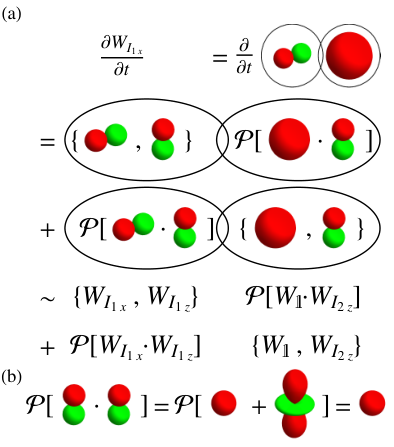
Here, the Poisson brackets from Eq. (8) gain an additional index in order to identify their spin dependence, i.e., the Poisson bracket $\{f_{a},f_{b}\}^{\{1\}}$ contains derivatives with respect to the variables $\theta_{1}$ and $\phi_{1}$ , while $\{f_{a},f_{b}\}^{\{2\}}$ is defined with reference to $\theta_{2}$ and $\phi_{2}$ . As spherical harmonics with rank two or higher are not allowed for spins $1/2$ , the projector $\mathcal{P}^{\{1,2\}}$ removes these superfluous contributions, but leaves spherical harmonics $\mathrm{Y}_{jm}$ with rank $j$ equal to zero or one unchanged. The Poisson brackets in Eq. (15) can be simplified for product operators $W_{\rho}=W_{\rho_{1}}(\theta_{1},\phi_{1})W_{\rho_{2}}(\theta_{2},\phi_{2})$ and $W_{\mathcal{H}}=W_{\mathcal{H}_{1}}(\theta_{1},\phi_{1})W_{\mathcal{H}_{2}}(\theta_{2},\phi_{2})$ into the form

\partial W_{\rho}/\partial t=\sqrt{2\pi}\,\{W_{\rho_{1}},W_{\mathcal{H}_{1}}\}^{\{1\}}\mathcal{P}^{\{2\}}(W_{\rho_{2}}W_{\mathcal{H}_{2}})+\sqrt{2\pi}\,\{W_{\rho_{2}},W_{\mathcal{H}_{2}}\}^{\{2\}}\mathcal{P}^{\{1\}}(W_{\rho_{1}}W_{\mathcal{H}_{1}});

(16)

refer to Figure 4(a) for a visualization of this computation. In the PROPS representation, product operators are indicated as overlapping circles (refer also to B) and the overall Wigner function of a tensor product $W_{1,2}=W_{1}W_{2}$ is given as a product of its parts. The corresponding Wigner functions $W_{1}$ is drawn in the left circle and the Wigner functions $W_{2}$ in the right one.

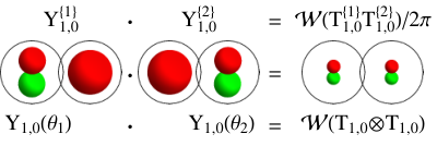
Using aforementioned techniques, the Hamiltonian and the deviation density matrix from Eqs. (11)-(12) can be transformed into their respective Wigner function

	$\displaystyle W_{\mathcal{H}}=4\pi^{2}\nu\,\mathrm{Y}^{\{1\}}_{10}\mathrm{Y}^{\{2\}}_{10}=\pi\nu 2R^{2}\cos{\theta_{1}}\cos{\theta_{2}},$		(17)
	$\displaystyle W_{\rho}(0)=(\mathrm{Y}^{\{1\}}_{1,-1}-\mathrm{Y}^{\{1\}}_{1,1})/\sqrt{2}=R\sin{\theta_{1}}\cos{\phi_{1}}/\sqrt{2\pi}.$		(18)

The time derivative of the initial Wigner function $W_{\rho}(0)$ is now given by Eq. (15) and it depends only on the variables $\theta_{1},\phi_{1}$ , consequently, the second Poisson bracket $\{W_{\rho}(0),W_{\mathcal{H}}\}^{\{2\}}$ is zero. One applies Eq. (8) and obtains up to projections

$\displaystyle\partial W_{\rho}(0)/\partial t$	$\displaystyle=\sqrt{2\pi}\{W_{\rho}(0),W_{\mathcal{H}}\}^{\{1\}}=\pi\nu 2R^{3}\{\sin{\theta_{1}}\cos{\phi_{1}},\cos{\theta_{1}}\}^{\{1\}}\cos{\theta_{2}}$
	$\displaystyle=\pi\nu 2R^{3}[\sin{\theta_{1}}\frac{\partial\cos{\phi_{1}}}{\partial\phi_{1}}\frac{\partial\cos{\theta_{1}}}{\partial\theta_{1}}]\cos{\theta_{2}}/(R\sin{\theta_{1}})$
	$\displaystyle=\pi\nu 2R^{2}\cos{\theta_{2}}\sin{\theta_{1}}\sin{\phi_{1}}=\pi\nu\mathcal{W}(2I_{1y}I_{2z}).$	(19)

Here, $\mathcal{W}(2I_{1y}I_{2z})$ denotes the Wigner transformation of $2I_{1y}I_{2z}$ , refer to Table 3. For the graphical representation of this computation refer to Figure 4(a). One deduces that the time derivative of $\mathcal{W}(2I_{1y}I_{2z})$ is up to projections proportional to

	$\displaystyle\partial^{2}W_{\rho}(0)/\partial t^{2}\propto\partial(\cos{\theta_{2}}\sin{\theta_{1}}\sin{\phi_{1}})/\partial t$
	$\displaystyle\propto\{\sin{\theta_{1}}\sin{\phi_{1}},\cos{\theta_{1}}\}^{\{1\}}\cos{\theta_{2}}\cos{\theta_{2}}+\cos{\theta_{1}}\sin{\theta_{1}}\sin{\phi_{1}}\{\cos{\theta_{2}},\cos{\theta_{2}}\}^{\{2\}}.$

Since $\{\cos{\theta_{2}},\cos{\theta_{2}}\}^{\{2\}}=0$ and $\{\sin{\theta_{1}}\sin{\phi_{1}},\cos{\theta_{1}}\}^{\{1\}}=-\sin{\theta_{1}}\cos{\phi_{1}}\sin{\theta_{1}}/(R\sin{\theta_{1}})$ , we obtain up to projections that

\partial\mathcal{W}(2I_{1y}I_{2z})/\partial t=-2\sqrt{3}R^{2}\pi\nu\sin{\theta_{1}}\cos{\phi_{1}}\cos^{2}{\theta_{2}}.

It is however important to understand that the term

\cos^{2}{\theta_{2}}=[\sqrt{4\pi}\mathrm{Y}_{00}(\theta_{2},\phi_{2})+4\sqrt{\pi/5}\>\mathrm{Y}_{20}(\theta_{2},\phi_{2})]/3

(20)

linearly decomposes into spherical harmonics of rank zero and two, as shown in Figure 4(b). After applying the projector $\mathcal{P}^{\{2\}}$ from Eq. (16), only a term proportional to $\mathrm{Y}_{00}=1/\sqrt{4\pi}$ remains;¹³¹³ 13 The term $\cos^{2}{\theta_{2}}$ is proportional to $\mathcal{W}(I_{2z})\mathcal{W}(I_{2z})$ . Note that in general $\mathcal{P}^{\{k\}}\mathcal{W}(I_{ka})\mathcal{W}(I_{kb})=\delta_{ab}/[4(2\pi)^{N}]$ with $a,b\in\{x,y,z\}$ holds for the pointwise product of Wigner functions, where $N$ denotes the number of spins $1/2$ . and this leads to

\partial\mathcal{W}(2I_{1y}I_{2z})/\partial t=-\tfrac{2R^{2}\pi\nu}{\sqrt{3}}\sin{\theta_{1}}\cos{\phi_{1}}=\mathcal{W}(-\pi\nu I_{1x}).

It is now apparent, that the second time derivative of $W_{\rho}(0)$ is proportional to $W_{\rho}(0)$ , i.e., $\partial^{2}W_{\rho}(0)/\partial t^{2}=-(\pi\nu)^{2}W_{\rho}(0)$ and that the time evolution of $W_{\rho}$ is parametrized by only two Wigner functions

W_{A}:=\mathcal{W}(I_{1x})=R\sin{\theta_{1}}\cos{\phi_{1}}/\sqrt{2\pi},\quad W_{B}:=\mathcal{W}(2I_{1y}I_{2z})=2R^{2}\sin{\theta_{1}}\sin{\phi_{1}}\cos{\theta_{2}}.

Note the similarity with Eq. (13). The solution for the Wigner function is then given by¹⁴¹⁴ 14 The parametrized Wigner function $W_{\rho}(t)=a(t)W_{A}+b(t)W_{B}$ is substituted into Eq. (15), and one obtains $\partial[a(t)W_{A}+b(t)W_{B}]/\partial t=\pi\nu[a(t)W_{B}-b(t)W_{A}]$ . This splits into $\partial a(t)/\partial t=-\pi\nu b(t)$ and $\partial b(t)/\partial t=\allowbreak{}\pi\nu a(t)$ and results in $W_{\rho}(t)=\cos(\pi\nu t)W_{A}+\sin(\pi\nu t)W_{B}$ .

W_{\rho}(t)=R\,c(t)\sin{\theta_{1}}\cos{\phi_{1}}/\sqrt{2\pi}+2R^{2}s(t)\sin{\theta_{1}}\sin{\phi_{1}}\cos{\theta_{2}},

(21)

where $c(t):=\cos(\pi\nu t)$ and $s(t):=\sin(\pi\nu t)$ . Figure 5 illustrates the time evolution of Wigner functions for the Hamiltonian $\mathcal{H}=\pi\nu 2I_{1z}I_{2z}$ (upper row), the traceless deviation density matrix $\rho(t)=c(t)I_{1x}+s(t)2I_{1y}I_{2z}$ (middle row), and the corresponding time derivative $\partial\rho/\partial t=-s(t)I_{1x}+c(t)2I_{1y}I_{2z}$ (lower row) at different times $t=0$ , $\pi\nu t=\pi/4$ , and $\pi\nu t=\pi/2$ . Arbitrary operators are visualized in the PROPS representation by decomposing them into sums of product operators (refer also to B). An alternative representation of the Wigner function in Eq. (21) based on a decomposition into non-hermitian operators is given in Sec. 5.4.2.

3 Theory: Wigner formalism for the time evolution of coupled spins

The central parts of the Wigner formalism for coupled spins are now systematically developed. Most of our theoretical concepts were already introduced in Sec. 2 using easily understandable examples. We present now the mathematical details for our Wigner formalism for coupled spins which form the main results of this work. Identifying the underlying physical principles, the description of the time evolution of coupled spin systems is consequently derived via our theoretical approach.

We want to emphasize that our theoretical approach, which relies on the irreducible tensor operators is applicable to arbitrary density matrices and operators of coupled spin systems, even though our technical tools (including Clebsch-Gordan coefficients and Wigner $6$ - $j$ symbols [70]) might spuriously suggest some superficial similarity to the description of indistinguishable particles using reducible representations of the special unitary group of dimension two. In particular, the star product specifying the time evolution is not determined by a simple addition of angular momenta, not even for a single spin [cf. Eq. (52) below].

First, we recall basic properties of product operators and the tensor product of matrices (see Sec. 3.1); the main properties are summarized in Table 4. We detail the Wigner transformation of spin operators for single and coupled spin systems in Sec. 3.2. This then leads in Sec. 3.3 to a simplified approach to compute the star product of single-spin-1/2 operators and allows us to derive the corresponding equation of motion. In Sec. 3.4, the star product is then extended to coupled spin- $1/2$ operators and the corresponding equation of motion is determined. Finally, we provide an optimized form of our formalism for two and three coupled spins $1/2$ as well as natural Hamiltonians for multiple spins $1/2$ (see Sec. 3.5).

Table 4: Normalized product operators and tensor products for basis operators embedded into an

N

-spin system; see also A. The names in the first column refer to the case when all indices

j_{k}>0

; but the prefactors are correct even if some

j_{k}

are zero.

Type	Product-operator notation	Tensor-product notation
Linear	${}^{\scriptstyle J}\mathrm{T}^{\{k\}}_{jm}$	$\underbrace{{}^{\scriptstyle J}\mathrm{T}_{00}}_{\#1}\otimes\>\cdots\otimes{}^{\scriptstyle J}\mathrm{T}_{00}\otimes\underbrace{{}^{\scriptstyle J}\mathrm{T}_{jm}}_{\#k}\otimes\>{}^{\scriptstyle J}\mathrm{T}_{00}\otimes\cdots\otimes\underbrace{{}^{\scriptstyle J}\mathrm{T}_{00}}_{\#N}$
Bilinear	$\sqrt{2J{+}1}^{N}{}^{\scriptstyle J}\mathrm{T}^{\{k\}}_{j_{k}m_{k}}{}^{\scriptstyle J}\mathrm{T}^{\{\ell\}}_{j_{\ell}m_{\ell}}$	$\underbrace{{}^{\scriptstyle J}\mathrm{T}_{00}}_{\#1}\otimes\>\cdots\otimes\underbrace{{}^{\scriptstyle J}\mathrm{T}_{j_{k}m_{k}}}_{\#k}\otimes\>\cdots\otimes\underbrace{{}^{\scriptstyle J}\mathrm{T}_{j_{\ell}m_{\ell}}}_{\#\ell}\otimes\>\cdots\otimes\underbrace{{}^{\scriptstyle J}\mathrm{T}_{00}}_{\#N}$
$M$ -linear	$\sqrt{2J{+}1}^{N(M-1)}$	$\bigotimes_{k\in\{1,\ldots,N\}}A_{k},$
	$\times\prod_{k\in K,\|K\|=M}{}^{\scriptstyle J}\mathrm{T}^{\{k\}}_{j_{k}m_{k}}$	$\text{where }A_{k}:=\begin{cases}{}^{\scriptstyle J}\mathrm{T}_{j_{k}m_{k}}&\text{if }k\in K,\\ {}^{\scriptstyle J}\mathrm{T}_{00}&\text{otherwise.}\end{cases}$
$N$ -linear	$\sqrt{2J{+}1}^{N(N-1)}$	${}^{\scriptstyle J}\mathrm{T}_{j_{1}m_{1}}\otimes\cdots\otimes{}^{\scriptstyle J}\mathrm{T}_{j_{N}m_{N}}$
	$\times{}^{\scriptstyle J}\mathrm{T}^{\{1\}}_{j_{1}m_{1}}\cdots{}^{\scriptstyle J}\mathrm{T}^{\{N\}}_{j_{N}m_{N}}$

3.1 Product-operator and tensor-product notation

We recapitulate elementary definitions and properties of tensor operators acting on a coupled $N$ -spin system consisting of spin- $J$ particles. For single spins, the tensor components ${}^{\scriptstyle J}\mathrm{T}_{jm}$ are indexed with rank $j\in\{0,\ldots,2J\}$ and order $m\in\{-j,\ldots,j\}$ ; the index $J$ can be dropped if $J=1/2$ . Recall the defining relations of tensor operators in Eq. (4), and their matrix elements given in the standard basis $|Jm\rangle$ can be specified in terms of Clebsch-Gordan coefficients [70, 24, 71, 72]

[{}^{\scriptstyle J}\mathrm{T}_{jm}]_{m_{1}m_{2}}:=\langle Jm_{1}|{}^{\scriptstyle J}\mathrm{T}_{jm}|Jm_{2}\rangle=\sqrt{\tfrac{2j{+}1}{2J{+}1}}\,C^{Jm_{1}}_{Jm_{2},jm}=(-1)^{J-m_{2}}\,C^{jm}_{Jm_{1}J,-m_{2}},

(22)

where $m_{1},m_{2}\in\{J,\ldots,-J\}$ . The single-spin operator ${}^{\scriptstyle J}\mathrm{T}_{jm}$ is normalized and can be embedded as the product operator

{}^{\scriptstyle J}\mathrm{T}^{\{k\}}_{jm}:={}^{\scriptstyle J}\mathrm{T}_{00}\otimes\cdots\otimes{}^{\scriptstyle J}\mathrm{T}_{00}\otimes{}^{\scriptstyle J}\mathrm{T}_{jm}\otimes{}^{\scriptstyle J}\mathrm{T}_{00}\otimes\cdots\otimes{}^{\scriptstyle J}\mathrm{T}_{00}

(23)

acting on the $k$ th spin of an $N$ -spin system (recall that $\mathbbmss{1}_{2J{+}1}=\sqrt{2J{+}1}\>{}^{\scriptstyle J}\mathrm{T}_{00}$ ). More generally, the embedded form of a single-spin operator $A$ acting on the $k$ th spin is denoted by $A^{\{k\}}:={}^{\scriptstyle J}\mathrm{T}_{00}\otimes\cdots\otimes{}^{\scriptstyle J}\mathrm{T}_{00}\otimes A\otimes{}^{\scriptstyle J}\mathrm{T}_{00}\otimes\cdots\otimes{}^{\scriptstyle J}\mathrm{T}_{00}$ . We consider products of single-spin tensor operators, and certain cases are summarized in Table 4 as normalized product operators $A$ with $\tr(A^{\dagger}A)=1$ , Table 4 also shows the complementary tensor-product notation, and we will switch between product operators and the tensor-product notation. Elementary properties of product operators can usually directly be inferred from properties of tensor products of operators $A_{k}$ and $B_{k}$ with $k\in\{1,\ldots,N\}$ :

	$\displaystyle(A_{1}\cdots A_{N})\otimes(B_{1}\cdots B_{N})=(A_{1}{\otimes}B_{1})\>\cdots\>(A_{N}{\otimes}B_{N}),\;(A_{1}\otimes\cdots\otimes A_{N})^{\dagger}=A_{1}^{\dagger}\otimes\cdots\otimes A_{N}^{\dagger},$
	$\displaystyle\text{and }\;\tr(A_{1}\otimes\cdots\otimes A_{N})=\tr(A_{1})\>\cdots\>\tr(A_{N}).$

Moreover, we gather the following properties of embedded single-spin product operators:

Lemma 1.

Embedded single-spin product operators have the following properties:

		$\displaystyle\text{{(a)}}\;\tr[({}^{\scriptstyle J}\mathrm{T}^{\{k_{1}\}}_{j_{1}m_{1}})^{\dagger}{}^{\scriptstyle J}\mathrm{T}^{\{k_{2}\}}_{j_{2}m_{2}}]=\delta_{k_{1}k_{2}}\delta_{j_{1}j_{2}}\delta_{m_{1}m_{2}},$
		$\displaystyle\text{{(b)}}\;[{}^{\scriptstyle J}\mathrm{T}^{\{k_{1}\}}_{j_{1}m_{1}},{}^{\scriptstyle J}\mathrm{T}^{\{k_{2}\}}_{j_{2}m_{2}}]=\tfrac{\delta_{k_{1}k_{2}}}{\sqrt{2J{+}1}^{N{-}1}}([{}^{\scriptstyle J}\mathrm{T}_{j_{1}m_{1}},{}^{\scriptstyle J}\mathrm{T}_{j_{2}m_{2}}])^{\{k_{1}\}},$
		$\displaystyle\text{{(c)}}\;{}^{\scriptstyle J}\mathrm{T}^{\{k\}}_{j_{1}m_{1}}{}^{\scriptstyle J}\mathrm{T}^{\{k\}}_{j_{2}m_{2}}=\tfrac{1}{\sqrt{2J{+}1}^{N{-}1}}({}^{\scriptstyle J}\mathrm{T}_{j_{1}m_{1}}{}^{\scriptstyle J}\mathrm{T}_{j_{2}m_{2}})^{\{k\}}.$

These properties imply that normalized products of single-spin tensor operators give rise to a basis of the full operator space of $N$ spins (cf. Table 4):

Lemma 2.

The normalized product operators

\sqrt{2J{+}1}^{N(N-1)}{}^{\scriptstyle J}\mathrm{T}^{\{1\}}_{j_{1}m_{1}}\cdots{}^{\scriptstyle J}\mathrm{T}^{\{N\}}_{j_{N}m_{N}}={}^{\scriptstyle J}\mathrm{T}_{j_{1}m_{1}}\otimes\cdots\otimes{}^{\scriptstyle J}\mathrm{T}_{j_{N}m_{N}}

form an orthonormal basis of the full $N$ -spin system, and an arbitrary spin operator $A$ can be decomposed as

A=\hskip-11.38109pt\sum_{j_{1}m_{1}\ldots j_{N}m_{N}}\hskip-11.38109pta_{j_{1}m_{1}\ldots j_{N}m_{N}}\sqrt{2J{+}1}^{N(N-1)}{}^{\scriptstyle J}\mathrm{T}^{\{1\}}_{j_{1}m_{1}}\cdots{}^{\scriptstyle J}\mathrm{T}^{\{N\}}_{j_{N}m_{N}}.

Given an $M$ -linear operator acting on $M\leq N$ spins, all indices $j_{k}$ in the decomposition of $A$ given in Lemma 2 are greater equal to zero for $k\in\{1,\ldots,N\}$ . Yet, certain indices $j_{k}$ have to be zero if $M<N$ . A provides a non-technical tutorial on elementary properties of product operators.

3.2 The Wigner formalism for spins

We describe the Wigner representation of spin operators which are mapped by the Wigner transformation to spherical functions. This bijective mapping fulfills the so-called Stratonovich postulates (and generalizations thereof) which are discussed in C for single spins as well as multiple coupled spins.

3.2.1 Wigner representation of single spins

The continuous Wigner representation of an arbitrary operator $A$ acting on a single spin $J$ is defined as [22]

\mathcal{W}(A):=W_{A}(\theta,\phi)=\tr[\Delta_{J}(\theta,\phi)A],

(24)

where $\mathcal{W}(A)$ denotes the Wigner transform of $A$ . In Eq. (24), we have used the kernel $\Delta_{J}(\theta,\phi)$ for a single spin $J$ which maps spin operators onto spherical functions, and it is given by¹⁵¹⁵ 15 We verify that $\Delta_{J}(\theta,\phi)=\sum_{j=0}^{2J}\sum_{m=-j}^{j}\mathrm{Y}^{*}_{j,-m}\>{}^{\scriptstyle J}\mathrm{T}_{j,-m}=\Delta_{J}^{\dagger}(\theta,\phi)$ is hermitian by using the Condon-Shortley phase convention and $\Delta_{J}^{\dagger}(\theta,\phi)=\sum_{j=0}^{2J}\sum_{m=-j}^{j}\mathrm{Y}_{jm}\>{}^{\scriptstyle J}\mathrm{T}^{\dagger}_{jm}$ .

\Delta_{J}(\theta,\phi):=\sum_{j=0}^{2J}\sum_{m=-j}^{j}\mathrm{Y}^{*}_{jm}(\theta,\phi)\>{}^{\scriptstyle J}\mathrm{T}_{jm}=\Delta_{J}^{\dagger}(\theta,\phi).

(25)

The form of the kernel builds on the work of [21, 22, 24, 23], see, in particular, Eqs. (4.16)-(4.17) in [24], Eq. 2.14 in [22], and Eq. (9) in [25]. Here, the tensor operators ${}^{\scriptstyle J}\mathrm{T}_{jm}$ for a given spin number $J$ form an orthonormal set of basis operators for $(2J{+}1)\times(2J{+}1)$ matrices, i.e.,

\tr({}^{\scriptstyle J}\mathrm{T}_{j_{1}m_{1}}^{\dagger}{}^{\scriptstyle J}\mathrm{T}_{j_{2}m_{2}})=\delta_{j_{1}j_{2}}\delta_{m_{1}m_{2}};

(26)

likewise the spherical harmonics $\mathrm{Y}_{jm}(\theta,\phi)$ [41] are orthonormal with respect to the scalar product

\int_{\theta=0}^{\pi}\int_{\phi=0}^{2\pi}\mathrm{Y}^{*}_{j_{1}m_{1}}(\theta,\phi)\mathrm{Y}_{j_{2}m_{2}}(\theta,\phi)\sin{\theta}\,\mathrm{d}\theta\,\mathrm{d}\phi=\delta_{j_{1}j_{2}}\delta_{m_{1}m_{2}}.

(27)

Equations (24) and (26) imply that the Wigner representation of a tensor operator ${}^{\scriptstyle J}\mathrm{T}_{jm}$ is equal to the spherical harmonic $\mathrm{Y}_{jm}(\theta,\phi)$ , i.e.,

\mathcal{W}({}^{\scriptstyle J}\mathrm{T}_{jm})=W_{{}^{\scriptstyle J}\mathrm{T}_{jm}}(\theta,\phi)=\mathrm{Y}_{jm}(\theta,\phi).

(28)

Tensor operators can be reconstructed from their Wigner representation by applying the inverse Wigner transformation (usually referred to as the Weyl transformation) which is defined as

\mathcal{W}^{-1}[F(\theta,\phi)]:=\int_{\theta=0}^{\pi}\int_{\phi=0}^{2\pi}\Delta_{J}(\theta,\phi)F(\theta,\phi)\>\sin{\theta}\,\mathrm{d}\theta\,\mathrm{d}\phi.

(29)

By substituting $F=W_{A}$ in Eq. (29), one obtains that $A=\mathcal{W}^{-1}[W_{A}(\theta,\phi)]$ . The orthonormality relation of Eq. (27) implies that the inverse Wigner transformation of the spherical harmonics ${\mathrm{Y}_{jm}(\theta,\phi)}$ are given by the tensor operators ${}^{\scriptstyle J}\mathrm{T}_{jm}$ .

3.2.2 Wigner representation of coupled spins

We now generalize the definition of the kernel for a single spin [see Eq. (25)] to multiple spins $J$ , but for simplicity with identical $J$ for each spin, while a generalization to systems that are composed of particles of different spin number $J$ is straightforward.

Result 1.

For $N$ coupled spins, the kernel is defined as the $N$ -fold tensor product

\Delta^{\{1\ldots N\}}_{J}:=\Delta^{\{1\ldots N\}}_{J}(\theta_{1},\phi_{1},\ldots,\theta_{N},\phi_{N})=\bigotimes_{k=1}^{N}\Delta_{J}(\theta_{k},\phi_{k})

of the individual kernels and involves a set of $2N$ variables $(\theta_{1},\phi_{1},\ldots,\theta_{N},\phi_{N})$ describing points on $N$ spheres.¹⁶¹⁶ 16 A similar result has been attained in Eq. (9) of [27]. Using the definition of the kernel $\Delta_{J}(\theta,\phi)$ from Eq. (25) and applying the correspondence of Table 4, one obtains the explicit form

	$\displaystyle\Delta^{\{1\dots N\}}_{J}$	$\displaystyle=\sum_{\begin{subarray}{c}j_{1}\dots j_{N}\\ m_{1}\dots m_{N}\end{subarray}}[{}^{\scriptstyle J}\mathrm{T}_{j_{1}m_{1}}\otimes\cdots\otimes{}^{\scriptstyle J}\mathrm{T}_{j_{N}m_{N}}]\;\mathcal{Y}$
		$\displaystyle=\sum_{\begin{subarray}{c}j_{1}\dots j_{N}\\ m_{1}\dots m_{N}\end{subarray}}[\sqrt{2J{+}1}^{N(N-1)}{}^{\scriptstyle J}\mathrm{T}^{\{1\}}_{j_{1}m_{1}}\cdots{}^{\scriptstyle J}\mathrm{T}^{\{N\}}_{j_{N}m_{N}}]\;\mathcal{Y},$		(30)

where $\mathcal{Y}:=\prod_{k=1}^{N}\mathrm{Y}^{*}_{j_{k}m_{k}}(\theta_{k},\phi_{k})$ . Consequently, this defines the Wigner transformation as

\mathcal{W}(A):=W_{A}(\theta_{1},\phi_{1},\ldots,\theta_{N},\phi_{N})=\tr(\Delta^{\{1\dots N\}}_{J}A),

(31)

and it satisfies the generalized Stratonovich postulates described in C.2.

We now apply orthonormality properties of tensor operators [see Lemma 1(a)] and verify that the Wigner representation for the linear embedded tensor operator ${}^{\scriptstyle J}\mathrm{T}^{\{k\}}_{jm}$ is proportional to the spherical harmonic $\mathrm{Y}_{jm}(\theta_{k},\phi_{k})$ , which depends on the angular variables $\theta_{k}$ and $\phi_{k}$ . More precisely, we obtain the relation

\mathcal{W}({}^{\scriptstyle J}\mathrm{T}^{\{k\}}_{jm})=\mathrm{Y}^{\{k\}}_{jm}:=\underbrace{\mathrm{Y}_{00}}_{\#1}\cdots\hskip-5.69054pt\underbrace{\mathrm{Y}_{00}}_{\#(k-1)}\underbrace{\mathrm{Y}_{jm}(\theta_{k},\phi_{k})}_{\#k}\underbrace{\mathrm{Y}_{00}}_{\#(k+1)}\hskip-5.69054pt\cdots\underbrace{\mathrm{Y}_{00}}_{\#N}\phantom{:}=\mathrm{Y}_{jm}(\theta_{k},\phi_{k})/\sqrt{4\pi}^{N-1}.

(32)

Similarly as for the Wigner transformation, the inverse Wigner transformation of a spherical function $F=F(\theta_{1},\phi_{1},\ldots,\theta_{N},\phi_{N})$ is generalized to multiple spins as

\mathcal{W}^{-1}(F):=\hskip-2.84526pt\idotsint\displaylimits_{\theta_{k},\phi_{k}\geq 0}^{\theta_{k}\leq\pi,\phi_{k}\leq 2\pi}\hskip-2.84526pt\Delta^{\{1\dots N\}}_{J}F\prod_{k=1}^{N}\sin{\theta_{k}}\,\mathrm{d}\phi_{k}\,\mathrm{d}\theta_{k}.

(33)

Setting $F=W_{A}$ in Eq. (33) also verifies that $A=\mathcal{W}^{-1}[W_{A}(\theta_{1},\phi_{1}\dots\theta_{N},\phi_{N})]$ holds. In particular, the inverse Wigner transformation maps the spherical harmonic $\mathrm{Y}_{jm}^{\{k\}}$ with variables $(\theta_{k},\phi_{k})$ to the linear tensor operators ${}^{\scriptstyle J}\mathrm{T}_{jm}^{\{k\}}$ acting on the $k$ th spin. Finally, our approach establishes that the Wigner representation of products of embedded tensor operators can be written as products of the corresponding spherical harmonics involving different variables, i.e.,

	$\displaystyle\mathcal{W}(\sqrt{2J{+}1}^{N(N-1)}\>{}^{\scriptstyle J}\mathrm{T}_{j_{1}m_{1}}^{\{1\}}\cdots\>{}^{\scriptstyle J}\mathrm{T}_{j_{N}m_{N}}^{\{N\}})$	$\displaystyle=\mathcal{W}(\>{}^{\scriptstyle J}\mathrm{T}_{j_{1}m_{1}}\otimes\cdots\otimes{}^{\scriptstyle J}\mathrm{T}_{j_{N}m_{N}})$		(34)
		$\displaystyle=\mathrm{Y}_{j_{1}m_{1}}(\theta_{1},\phi_{1})\>\cdots\>\mathrm{Y}_{j_{N}m_{N}}(\theta_{N},\phi_{N}).$

3.2.3 Star product, star commutator, and Moyal equation

In the following, we wish to compute the Wigner representation $W_{AB}$ of the product $AB$ of two operators $A$ and $B$ from their respective Wigner representations $W_{A}$ and $W_{B}$ . This is accomplished by recalling the defining relation

W_{AB}=W_{A}\star W_{B}

(35)

of the star product $\star$ of two Wigner functions. The star product mimics the matrix product of two operators. Note that the product $AB$ is restricted to the subspace of tensor operators with rank at most $2J$ , just as for the operators $A$ and $B$ .

The time evolution of the density operator $\rho$ is governed by the von-Neumann equation $i\partial\rho/\partial t=[\mathcal{H},\rho]=\mathcal{H}\rho-\rho\mathcal{H}$ , see Eq. (1). This can be mapped to the Wigner representation by applying Eq. (24) and exploiting that the symbols $W_{\rho\mathcal{H}}$ and $W_{\mathcal{H}\rho}$ can according to Eq. (35) be restated in terms of star products. Hence, the equation of motion in the Wigner representation is given as

i\frac{\partial W_{\rho}}{\partial t}=[W_{\mathcal{H}},W_{\rho}]_{\star}:=W_{\mathcal{H}}\star W_{\rho}-W_{\rho}\star W_{\mathcal{H}}.

(36)

This defines the star commutator $[\cdot,\cdot]_{\star}$ , which constitutes an analogue of the matrix commutator.

3.3 Star product for a single spin $1/2$

Wigner representations and their defining star products are well studied in the case of infinite-dimensional quantum-mechanical operators [15, 16]. Similarly as in the infinite-dimensional case, the star product from Eq. (35) can be computed using an integral or differential form (as discussed in Sections 1.2 and 1.5.1). The integral form is an integral transformation of the Wigner functions $W_{A}(\theta_{1},\phi_{1})$ and $W_{B}(\theta_{2},\phi_{2})$ which is weighted with a so-called trikernel. We provide an explicit expression for the integral form in Eq. (96) of F (along the lines of [22]) by evaluating the exact star product and by applying expansion formulas from Sec. 3.3.1 below. This result provides a formal definition of the star product, but is less useful in applications.

In contrast, the differential star product is more convenient for explicit calculations since only partial derivatives and the pointwise product of $W_{A}$ and $W_{B}$ are required, which is afterwards followed by a projection.

For an arbitrary spin number $J$ , Klimov and Espinoza [25] state the differential star product for two so-called Beresin P symbols $P_{A}$ and $P_{B}$ as a sum of the pointwise product of two functions combined with partial derivatives. The order and number of the partial derivatives grow rapidly with increasing $J$ , and a truncation of the resulting P symbol is required. Klimov and Espinoza [25] also provide formulas to compute the star product of Wigner functions. Their method is virtually equivalent to transforming the Wigner functions into P symbols, then after computing the star product of P symbols, the P symbols are transformed back. In summary, the star product of two spin- $1/2$ Wigner functions $W_{A}$ and $W_{B}$ can be computed by first decomposing $W_{A}$ and $W_{B}$ into spherical harmonics and by reweighting the expansion coefficients one obtains $\tilde{W}_{A}$ and $\tilde{W}_{B}$ , where $\tilde{W}_{A}$ and $\tilde{W}_{B}$ are proportional to the P symbols $P_{A}$ and $P_{B}$ . The differential star product of the P symbols is then applied to $\tilde{W}_{A}$ and $\tilde{W}_{B}$ , and one obtains the four summands $a\,\tilde{W}_{A}\tilde{W}_{B}$ , $b\,\{\tilde{W}_{A},\tilde{W}_{B}\}$ , $c\,(\partial\tilde{W}_{A}/\partial\theta)\,(\partial\tilde{W}_{B}/\partial\theta)$ , and $d\,(\partial\tilde{W}_{A}/\partial\phi)\,(\partial\tilde{W}_{B}/\partial\phi)/\sin^{2}{\theta}$ , where $a$ , $b$ , $c$ , and $d$ denote suitable prefactors. The resulting function $\tilde{W}_{AB}$ is transformed back by reweighting the terms in its decomposition into spherical harmonics. Finally, a result $W_{AB}$ is obtained that satisfies the defining property $W_{AB}=W_{A}\star W_{B}$ .

We consider only the case of $J=1/2$ and provide a simplified approach, which nevertheless leads to the same star product and the same equation of motion that is given by the Poisson bracket (see [30] and [22]). The resulting differential star product $W_{A}\star W_{B}$ [see Result 2 below] is simply a sum of the pointwise product $W_{A}W_{B}$ and the Poisson bracket $\{W_{A},W_{B}\}$ of the two Wigner functions. In Sec. 3.3.1 we provide formulas necessary to evaluate the star product, and Sec. 3.3.2 contains the details on how the star product is calculated. This simplified approach allows us then to extend the star product to multiple, coupled spins as detailed in Sec. 3.4.

3.3.1 Matrix products, pointwise products, and Poisson brackets

We detail how to expand products of tensor operators (resp. spherical harmonics) into a linear combination of tensor operators (resp. spherical harmonics). A similar expansion is described for the Poisson bracket of spherical harmonics. The product of two irreducible tensor operators can be expanded as [25, 73]

{}^{\scriptstyle J}\mathrm{T}_{j_{1}m_{1}}{}^{\scriptstyle J}\mathrm{T}_{j_{2}m_{2}}=\sum_{L=|j_{1}-j_{2}|}^{n}{}^{J}Q_{j_{1}j_{2}L}\,C^{LM}_{j_{1}m_{1}j_{2}m_{2}}{}^{\scriptstyle J}\mathrm{T}_{LM}.

(37)

Here, the upper bound of the summation does not need to exceed $2J$ and is given by $n:=\min(j_{1}{+}j_{2},2J)$ as ${}^{J}Q_{j_{1}j_{2}L}=0$ for $L>2J$ ; note $M=m_{1}{+}m_{2}$ .¹⁷¹⁷ 17 The lower bound in the summation can be enlarged to $\max(|j_{1}{-}j_{2}|,m_{1}{+}m_{2})$ without changing the result. Also, $C^{LM}_{j_{1}m_{1}j_{2}m_{2}}$ are the Clebsch-Gordan coefficients [70], and the coefficients

{}^{J}Q_{j_{1}j_{2}L}:=(-1)^{2J+L}\sqrt{(2j_{1}{+}1)(2j_{2}{+}1)}\>\begin{Bmatrix}j_{1}&j_{2}&L\\ J&J&J\end{Bmatrix}

(38)

are proportional to Wigner $6$ - $j$ symbols [70] and depend only on $j_{1}$ , $j_{2}$ , and $L$ , but are independent of $m_{1}$ , $m_{2}$ , and $M$ . This also conforms with the fact that only tensor operators of rank zero and one are allowed for the case of a spin $1/2$ in the product $AB$ (see Sec. 3.2.3).

In order to determine the Poisson bracket of two spherical functions, we first recall its definition [refer also to Eq. (8)]

\{W_{F},W_{G}\}^{\{i\}}:=W_{F}\left(\tfrac{\overleftarrow{\partial}}{\partial\phi_{i}}\tfrac{1}{R\sin\theta_{i}}\tfrac{\overrightarrow{\partial}}{\partial\theta_{i}}-\tfrac{\overleftarrow{\partial}}{\partial\theta_{i}}\tfrac{1}{R\sin\theta_{i}}\tfrac{\overrightarrow{\partial}}{\partial\phi_{i}}\right)W_{G},

(39)

where the arrows $\leftarrow$ and $\rightarrow$ indicate whether the derivatives act to the left or the right, respectively. Moreover, the normalization factor is set to $R=\sqrt{3/(8\pi)}$ . Based on [74], the Poisson bracket of two spherical harmonics can be expanded as

\{\mathrm{Y}_{j_{1}m_{1}},\mathrm{Y}_{j_{2}m_{2}}\}=\sum_{L=|j_{1}-j_{2}|}^{j_{1}+j_{2}}U_{j_{1}j_{2}L}\,C^{LM}_{j_{1}m_{1}j_{2}m_{2}}\mathrm{Y}_{LM}.

(40)

The product of two spherical harmonics decomposes into a linear combination as (see Sec. 12.9 of [75])

\mathrm{Y}_{j_{1}m_{1}}\mathrm{Y}_{j_{2}m_{2}}=\sum_{L=|j_{1}-j_{2}|}^{j_{1}+j_{2}}Z_{j_{1}j_{2}L}\,C^{LM}_{j_{1}m_{1}j_{2}m_{2}}\mathrm{Y}_{LM}.

(41)

Here, the coefficients $Z_{j_{1}j_{2}L}$ and $U_{j_{1}j_{2}L}$ depend only on $j_{1}$ , $j_{2}$ , and $L$ and are given by

	$\displaystyle Z_{j_{1}j_{2}L}:=$	$\displaystyle\,\sqrt{\tfrac{(2j_{1}{+}1)(2j_{2}{+}1)}{4\pi(2L{+}1)}}C_{j_{1}0j_{2}0}^{L0},$		(42)
	$\displaystyle U_{j_{1}j_{2}L}:=$	$\displaystyle-\tfrac{i}{2R}[1-(-1)^{L-j_{1}-j_{2}}]\sqrt{j_{1}(j_{1}{+}1)L(L{+}1)}\times\sqrt{\tfrac{(2j_{1}{+}1)(2j_{2}{+}1)}{4\pi(2L{+}1)}}C_{j_{1}1\,j_{2}\,0}^{L1}.$		(43)

Although the Poisson bracket $\{\cdot,\cdot\}$ will not be completely analogous to the star commutator $[\cdot,\cdot]_{\star}$ for arbitrary $J$ , there is a strong relation between these two operations. Recalling that the star commutator in the Wigner representation corresponds to the commutator of matrix representations (see Sec. 3.2.3), we can in analogy compare the Poisson bracket from Eq. (40) with the usual commutator of tensor operators. Using Eq. (37), the commutator of tensor operators can be brought into a similar form ( $M=m_{1}+m_{2}$ )

[{}^{\scriptstyle J}\mathrm{T}_{j_{1}m_{1}},{}^{\scriptstyle J}\mathrm{T}_{j_{2}m_{2}}]=\hskip-5.69054pt\sum_{L=|j_{1}-j_{2}|}^{n}\hskip-2.84526pt{}^{J}Q^{\prime}_{j_{1}j_{2}L}\,C^{LM}_{j_{1}m_{1}j_{2}m_{2}}{}^{\scriptstyle J}\mathrm{T}_{LM}

(44)

by applying ${}^{J}Q^{\prime}_{j_{1}j_{2}L}:=[1-(-1)^{j_{1}+j_{2}-L}]^{J}Q_{j_{1}j_{2}L}$ and the symmetry properties $C^{LM}_{j_{1}m_{1}j_{2}m_{2}}=(-1)^{j_{1}+j_{2}-L}C^{LM}_{j_{2}m_{2}j_{1}m_{1}}$ of the Clebsch-Gordan coefficients. We compare Eq. (40) with Eq. (44) and note that the coefficients $Q^{\prime(J)}_{j_{1}j_{2}L}$ and $U_{j_{1}j_{2}L}$ will in general differ. However, their nonzero values within the range $j_{1},j_{2},L\leq 2J$ appear at coinciding values of $j_{1}$ , $j_{2}$ , and $L$ , highlighting the close relation of the Poisson bracket and the star commutator. Finally, we provide a particular case where this equivalence is strict up to a prefactor:


$\displaystyle\{\mathrm{Y}_{10},\mathrm{Y}_{jm}\}$	$\displaystyle=i\sqrt{2}\>m\>\mathrm{Y}_{jm},$	$\displaystyle\{\mathrm{Y}_{1,\pm 1},\mathrm{Y}_{jm}\}$	$\displaystyle=\mp i\sqrt{\left(j\mp m\right)\left(j\pm m+1\right)}\>\mathrm{Y}_{j,m\pm 1},$	(45a)
$\displaystyle[^{J}\hskip-2.27621ptI_{z},{}^{\scriptstyle J}\mathrm{T}_{jm}]$	$\displaystyle=m\>{}^{\scriptstyle J}\mathrm{T}_{jm},$	$\displaystyle[^{J}\hskip-2.27621ptI_{\pm},{}^{\scriptstyle J}\mathrm{T}_{jm}]$	$\displaystyle=\sqrt{\left(j\mp m\right)\left(j\pm m+1\right)}\>{}^{\scriptstyle J}\mathrm{T}_{j,m\pm 1}.$	(45b)

The Equations (45b) show how the basic definition of spherical tensor operators relies on commutators, c.f. Eq. (4). By comparing them to the Equations (45a) it is clear that the defining relation is also satisfied by the Poisson bracket of spherical harmonics up to the prefactor $i$ (and an additional prefactor implied by $\mp N_{J}\mathcal{W}(^{J}\hskip-2.27621ptI_{\pm})=\mathrm{Y}_{1,\pm 1}$ and $N_{J}\sqrt{2}\mathcal{W}(^{J}\hskip-2.27621ptI_{z})=\mathrm{Y}_{1,0}$ ).¹⁸¹⁸ 18 The prefactor $N_{J}$ is implied by the formula ${}^{\scriptstyle J}\mathrm{T}_{1,\pm 1}=\mp^{J}\hskip-2.27621ptI_{\pm}N_{J}=\mp^{J}\hskip-2.27621ptI_{\pm}/\sqrt{\tr(^{J}\hskip-2.27621ptI_{\pm}\,^{J}\hskip-2.27621ptI_{\mp}})$ where ${}^{J}\hskip-2.27621ptI_{\pm}={}^{J}\hskip-2.27621ptI_{x}\pm i{}^{J}\hskip-2.27621ptI_{y}$ . The trace is given by $\tr(^{J}\hskip-2.27621ptI_{\pm}\,^{J}\hskip-2.27621ptI_{\mp})=\tr[({}^{J}\hskip-2.27621ptI_{x}\pm i{}^{J}\hskip-2.27621ptI_{y})({}^{J}\hskip-2.27621ptI_{x}\mp i{}^{J}\hskip-2.27621ptI_{y})]=\tr[^{J}\hskip-2.27621pt(I^{2})]-\tr[(^{J}\hskip-2.27621ptI_{z})^{2}]$ , where ${}^{J}\hskip-2.27621pt(I^{2})=(^{J}\hskip-2.27621ptI_{x})^{2}+(^{J}\hskip-2.27621ptI_{y})^{2}+(^{J}\hskip-2.27621ptI_{z})^{2}$ , $\tr[^{J}\hskip-2.27621pt(I^{2})]=J(J{+}1)(2J{+}1)$ , and $\tr[(^{J}\hskip-2.27621ptI_{z})^{2}]=\sum_{m=-J}^{J}m^{2}=J(J{+}1)(2J{+}1)/3$ . It follows that $N_{J}=1/\sqrt{\tr(^{J}\hskip-2.27621pt\,I_{\pm}^{J}\hskip-2.27621ptI_{\mp})}=1/\sqrt{2J(J{+}1)(2J{+}1)/3}$ . The particular cases of Eq. (45) are also considered in Equation (5.13) of [22].

3.3.2 Evaluation of the star product

In this section, we detail the explicit form of the differential star product for a single spin $1/2$ while ensuring that its form conforms with Sec. 3.2.3. We build on the work in [25, 22] and provide a simplified approach. The differential star product is given as the sum of the pointwise product and the Poisson bracket of two spherical functions, followed by the projection onto rank-one and rank-zero spherical harmonics, i.e., by truncating spherical harmonics with rank greater than one. Two distinct symbols are used: the exact star product $\star$ is obtained from the prestar product $\smallstar$ after truncating certain spherical harmonics.

Result 2.

Given the Wigner functions $W_{F}(\theta,\phi)$ and $W_{G}(\theta,\phi)$ of the operators $F$ and $G$ acting on a single spin $1/2$ , the prestar product (i.e., the product that results in the star product after truncation) is defined as

	$\displaystyle W_{F}(\theta,\phi)\smallstar W_{G}(\theta,\phi)$	$\displaystyle:=\sqrt{2\pi}W_{F}W_{G}{-}\tfrac{i}{2}\{W_{F},W_{G}\}$	(46)
using the Poisson bracket $\{\cdot,\cdot\}$ from Eq. (39). Note that the factor $\sqrt{2\pi}=1/W_{\mathbbmss{1}}$ is the inverse of the identity Wigner function. The corresponding star product
	$\displaystyle W_{F}(\theta,\phi)\star W_{G}(\theta,\phi)$	$\displaystyle:=\mathcal{P}[W_{F}(\theta,\phi)\smallstar W_{G}(\theta,\phi)]$	(47)

is obtained by projecting onto spherical functions of rank zero or one, e.g., by applying the projection operator

\mathcal{P}\,\mathrm{Y}_{jm}:=(1+\mathcal{L}^{2}/12-\mathcal{L}^{4}/24)\mathrm{Y}_{jm}=\begin{cases}\mathrm{Y}_{jm}\quad\textup{for}\quad j<2\\ 0\quad\textup{for}\quad j=2\end{cases}

(48)

which uses the angular momentum operator $\mathcal{L}$ with eigenvalues $\mathcal{L}^{2}\,\mathrm{Y}_{jm}=j(j{+}1)\mathrm{Y}_{jm}$ .¹⁹¹⁹ 19 The projector $\mathcal{P}f(\theta,\phi)=\sum_{j=0}^{1}\sum_{m=-j}^{j}\mathrm{Y}_{jm}(\theta,\phi)\int_{\theta=0}^{\pi}\int_{\phi=0}^{2\pi}f(\theta,\phi)\mathrm{Y}_{jm}^{*}(\theta,\phi)\>\sin{\theta}\,\mathrm{d}\theta\,\mathrm{d}\phi$ can be applied to an arbitrary spherical function, but Equation (47) is fulfilled by the differential operator in Equation (48).

We will now verify that this definition satisfies the defining property $W_{FG}(\theta,\phi)=W_{F}(\theta,\phi)\star W_{G}(\theta,\phi)$ of a star product [see Eq. (35)]. We start by expanding the operators $F=\sum_{j=0}^{1}\sum_{m=-j}^{j}f_{jm}\mathrm{T}_{jm}$ and $G=\sum_{j=0}^{1}\sum_{m=-j}^{j}g_{jm}\mathrm{T}_{jm}$ into tensor operators $\mathrm{T}_{jm}$ . One directly obtains that

FG=\sum_{j_{1},j_{2}=0}^{1}\sum_{m_{1}=-j_{1}}^{j_{1}}\sum_{m_{2}=-j_{2}}^{j_{2}}f_{j_{1}m_{1}}g_{j_{2}m_{2}}\>\mathrm{T}_{j_{1}m_{1}}\mathrm{T}_{j_{2}m_{2}}.

(49)

This summation involves products $\mathrm{T}_{j_{1}m_{1}}\mathrm{T}_{j_{2}m_{2}}$ of tensor operators which can be rewritten following Eq. (37) as

\mathrm{T}_{j_{1}m_{1}}\mathrm{T}_{j_{2}m_{2}}=\sum_{L=|j_{1}-j_{2}|}^{n}\,Q^{(1/2)}_{j_{1}j_{2}L}\,C^{LM}_{j_{1}m_{1}j_{2}m_{2}}\mathrm{T}_{LM},

(50)

where $n$ can be limited to $n=\min(j_{1}{+}j_{2},2J)$ and $M=m_{1}{+}m_{2}$ . In order to compare Eqs. (49) and (50) with their counterparts in the Wigner space, we also compute the star product $W_{F}(\theta,\phi)\star W_{G}(\theta,\phi)$ . Recall from Eq. (28) that the Wigner representations of $F$ and $G$ are given by $W_{F}=\sum_{j=0}^{1}\sum_{m=-j}^{j}f_{jm}\mathrm{Y}_{jm}$ and $W_{G}=\sum_{j=0}^{1}\sum_{m=-j}^{j}g_{jm}\mathrm{Y}_{jm}$ . The prestar product (i.e., the product that results in the star product after truncation) evaluates to

W_{F}(\theta,\phi)\smallstar W_{G}(\theta,\phi)=\sum_{j_{1},j_{2}=0}^{1}\sum_{m_{1}=-j_{1}}^{j_{1}}\sum_{m_{2}=-j_{2}}^{j_{2}}f_{j_{1}m_{1}}g_{j_{2}m_{2}}\,\mathrm{Y}_{j_{1}m_{1}}\smallstar\mathrm{Y}_{j_{2}m_{2}},

(51)

where the explicit formula of Eq. (46) results in

\mathrm{Y}_{j_{1}m_{1}}\smallstar\mathrm{Y}_{j_{2}m_{2}}=\sqrt{2\pi}\,\mathrm{Y}_{j_{1}m_{1}}\mathrm{Y}_{j_{2}m_{2}}-\tfrac{i}{2}\,\{\mathrm{Y}_{j_{1}m_{1}},\mathrm{Y}_{j_{2}m_{2}}\}=\sum_{L=|j_{1}-j_{2}|}^{j_{1}+j_{2}}{\Lambda_{j_{1}j_{2}L}}C^{LM}_{j_{1}m_{1}j_{2}m_{2}}\mathrm{Y}_{LM}.

(52)

Here, we have applied the formulas in Eqs. (40) and (41) and use the notation $\Lambda_{j_{1}j_{2}L}:=\sqrt{2\pi}Z_{j_{1}j_{2}L}-(i/2)U_{j_{1}j_{2}L}$ . The corresponding star product $\star$ is obtained if we substitute the upper summation bound in Eq. (52) with $n=\min(j_{1}{+}j_{2},2J)$ , which is the same bound as in Eq. (50). We are now ready to compare the tensor operators in Eqs. (49) and (50) with their respective complements in the Wigner space in Eqs. (51) and (52). Consequently, we have to compare the explicit values of the coefficients $Q^{(1/2)}_{j_{1}j_{2}L}$ and $\Lambda_{j_{1}j_{2}L}$ and we obtain that

		$\displaystyle Q^{(1/2)}_{000}=Q^{(1/2)}_{011}=Q^{(1/2)}_{101}=\Lambda_{000}=\Lambda_{011}=\Lambda_{101}=\tfrac{1}{\sqrt{2}},$
		$\displaystyle Q^{(1/2)}_{110}=\Lambda_{110}=-{\tfrac{\sqrt{3}}{\sqrt{2}}},\;Q^{(1/2)}_{111}=\Lambda_{111}=-1,$

and all other values are zero. This verifies that $\mathrm{Y}_{j_{1}m_{1}}\star\mathrm{Y}_{j_{2}m_{2}}=\mathcal{P}(\mathrm{Y}_{j_{1}m_{1}}\smallstar\mathrm{Y}_{j_{2}m_{2}})=\mathcal{W}(\mathrm{T}_{j_{1}m_{1}}\mathrm{T}_{j_{2}m_{2}})$ , and one respectively concludes that $W_{FG}(\theta,\phi)=W_{F}(\theta,\phi)\star W_{G}(\theta,\phi)$ . The preceding discussion is summarized as

Theorem 3.

The explicit form of the star product $\star$ in Eq. (47) observes its defining property from Eq. (35), i.e. $W_{FG}(\theta,\phi)=W_{F}(\theta,\phi)\star W_{G}(\theta,\phi)$ .

The explicit values for the prestar product $\smallstar$ (i.e., the product that results in the star product after truncation) for Wigner functions forming a basis for a single spin $1/2$ are presented in Table 5. The corresponding star product $\star$ is obtained by truncating the underlined parts in Table 5.

Table 5: Prestar product

\smallstar

(i.e., the product that results in the star product after truncation) of spherical harmonics for a single spin

1/2

. The corresponding star product

\star

is obtained by discarding the underlined components

\mathrm{Y}_{jm}

with

j>1

$\downarrow\smallstar\rightarrow$	$\mathrm{Y}_{00}$	$\mathrm{Y}_{1,-1}$	$\mathrm{Y}_{10}$	$\mathrm{Y}_{11}$
$\mathrm{Y}_{00}$	$\tfrac{1}{\sqrt{2}}\mathrm{Y}_{00}$	$\tfrac{1}{\sqrt{2}}\mathrm{Y}_{1,-1}$	$\tfrac{1}{\sqrt{2}}\mathrm{Y}_{10}$	$\tfrac{1}{\sqrt{2}}\mathrm{Y}_{11}$
$\mathrm{Y}_{1,-1}$	$\tfrac{1}{\sqrt{2}}\mathrm{Y}_{1,-1}$	$0\underline{{+}\sqrt{\tfrac{3}{5}}\mathrm{Y}_{2,-2}}$	$\tfrac{1}{\sqrt{2}}\mathrm{Y}_{1,-1}\underline{{+}\sqrt{\tfrac{3}{10}}\mathrm{Y}_{2,-1}}$	$-\tfrac{1}{\sqrt{2}}\mathrm{Y}_{00}{+}\tfrac{1}{\sqrt{2}}\mathrm{Y}_{10}$
				$\underline{{+}\tfrac{1}{\sqrt{10}}\mathrm{Y}_{20}}$
$\mathrm{Y}_{10}$	$\tfrac{1}{\sqrt{2}}\mathrm{Y}_{10}$	$-\tfrac{1}{\sqrt{2}}\mathrm{Y}_{1,-1}\underline{{+}\sqrt{\tfrac{3}{10}}\mathrm{Y}_{2,-1}}$	$\tfrac{1}{\sqrt{2}}\mathrm{Y}_{00}\underline{{+}\sqrt{\tfrac{2}{5}}\mathrm{Y}_{20}}$	$\tfrac{1}{\sqrt{2}}\mathrm{Y}_{11}\underline{{+}\sqrt{\tfrac{3}{10}}\mathrm{Y}_{21}}$
$\mathrm{Y}_{11}$	$\frac{1}{\sqrt{2}}\mathrm{Y}_{11}$	$-\tfrac{1}{\sqrt{2}}\mathrm{Y}_{00}{-}\tfrac{1}{\sqrt{2}}\mathrm{Y}_{10}$	$-\tfrac{1}{\sqrt{2}}\mathrm{Y}_{11}\underline{{+}\sqrt{\tfrac{3}{10}}\mathrm{Y}_{21}}$	$0\underline{{+}\sqrt{\tfrac{3}{5}}\mathrm{Y}_{22}}$
		$\underline{{+}\tfrac{1}{\sqrt{10}}\mathrm{Y}_{20}}$

3.3.3 Equation of motion based on the star product

We can now apply Result 2 to the differential equation given in Eq. (36) in order to provide its explicit form for a single spin $1/2$ . This results in the time evolution [22, 30]

\partial W_{A}/\partial t=\{W_{A},W_{\mathcal{H}}\}

(53)

in the Wigner space which is governed by the Poisson bracket. A detailed visualization of the whole structure of our formalism leading to Eq. (53) is given in Figure 9 of E. It can be inferred from Table 5 (as $\mathrm{Y}_{jm}$ with $j>1$ in the decomposition are symmetric with respect to the order of multiplication) that $\{W_{A},W_{B}\}=i(W_{A}{\star}W_{B}-W_{B}{\star}W_{A})=i(W_{A}{\smallstar}W_{B}-W_{B}{\smallstar}W_{A})$ holds for a single spin $1/2$ . This means that a truncation is not required to compute the time evolution in this particular case. In the case of Hamiltonians that contain only ${}^{J}\hskip-2.27621ptI_{x}$ , ${}^{J}\hskip-2.27621ptI_{y}$ and ${}^{J}\hskip-2.27621ptI_{z}$ in the form ${}^{J}\mathcal{H}=c_{x}\,^{J}\hskip-2.27621ptI_{x}+c_{y}\,^{J}\hskip-2.27621ptI_{y}+c_{z}\,^{J}\hskip-2.27621ptI_{z}$ Eq. (53) holds for arbitrary spin $J$ [up to a global prefactor $N_{J}$ as implied by Eq. (45)],¹⁸¹⁸footnotemark: 18 and agrees with the results of [22, 30]. Consequently, the time differential for an arbitrary spin $J$ evolving under a linear Hamiltonian is given as

\partial W_{{}^{J}\hskip-2.27621ptA}/\partial t=N_{J}\{W_{{}^{J}\hskip-2.27621ptA},W_{{}^{J}\mathcal{H}}\},

(54)

where $N_{J}$ is a global prefactor¹⁸¹⁸footnotemark: 18 and ${}^{J}\hskip-2.27621ptA$ denotes an arbitrary spin- $J$ operator.

3.4 Star product for multiple coupled spins with spin number $J=1/2$

We extend the star product from Result 2 to multiple coupled spins. To this end, we introduce a projection operator $\mathcal{P}^{\{1\ldots N\}}:=\prod_{k=1}^{N}\mathcal{P}^{\{k\}}$ which restricts resulting spherical harmonics to rank zero and one²⁰²⁰ 20 In general, an arbitrary, multivariate spherical function $f=f(\theta_{1},\phi_{1},\ldots,\theta_{N},\phi_{N})$ is projected using $\mathcal{P}^{\{k\}}f=\sum_{j_{k}=0}^{1}\sum_{m_{k}=-j_{k}}^{j_{k}}\mathrm{Y}_{j_{k}m_{k}}(\theta_{k},\phi_{k})\int_{\theta_{k}=0}^{\pi}\int_{\phi_{k}=0}^{2\pi}f\;\mathrm{Y}^{*}_{j_{k}m_{k}}(\theta_{k},\phi_{k})\sin{\theta_{k}}\,\mathrm{d}\phi_{k}\,\mathrm{d}\theta_{k}$ . and which can be via Equation (48) written as

\mathcal{P}^{\{k\}}:=(1+(\mathcal{L}^{\{k\}})^{2}/12-(\mathcal{L}^{\{k\}})^{4}/24).

(55)

The angular momentum operator $\mathcal{L}$ acts as $(\mathcal{L}^{\{k\}})^{2}\,\mathrm{Y}_{jm}(\theta_{k},\phi_{k})$ and has the eigenvalues $j(j{+}1)\mathrm{Y}_{jm}(\theta_{k},\phi_{k})$ . This projection will be used to truncate superfluous terms in the following definition of the star product:

Result 3.

The prestar product (the product that results in the star product after truncation) of two Wigner functions $W_{A}$ and $W_{B}$ corresponding to operators $A$ and $B$ in a system of $N$ coupled spins $1/2$ is defined as

W_{A}\smallstar W_{B}:=W_{A}(\prod_{k=1}^{N}\smallstar^{\{k\}})W_{B},

where the individual prestar operators are given by $\smallstar^{\{k\}}:=\sqrt{2\pi}-i\{\cdot,\cdot\}^{\{k\}}/2$ (cf. Result 2, Eq. (46)) and $\{\cdot,\cdot\}^{\{k\}}$ denotes the Poisson bracket taken with respect to the variables $\theta_{k}$ and $\phi_{k}$ , see Eq. (39). The star product

W_{A}\star W_{B}:=\mathcal{P}^{\{1\ldots N\}}(W_{A}\smallstar W_{B})\phantom{:}=\mathcal{P}^{\{1\ldots N\}}(W_{A}[\prod_{k=1}^{N}(\sqrt{2\pi}-\tfrac{i}{2}\{\cdot,\cdot\}^{\{k\}})]W_{B}).

(56)

is obtained by applying the projection operator $\mathcal{P}^{\{1\ldots N\}}$ .

The star product for coupled spins in Result 3 allows us to establish the form of the Wigner representation for multispin product operators $\mathrm{T}^{\{1\}}_{j_{1}m_{1}}\cdots\mathrm{T}^{\{N\}}_{j_{N}m_{N}}$ , which consists of matrix products of single-spin operators, cf. Table 4. In the Wigner representation, matrix products are substituted by star products:

Lemma 4.

The Wigner representation of product operators $\mathrm{T}^{\{1\}}_{j_{1}m_{1}}\cdots\mathrm{T}^{\{N\}}_{j_{N}m_{N}}$ is given by the prestar products (i.e., the product that results in the star product after truncation) of the Wigner representations $\mathcal{W}(\mathrm{T}^{\{k\}}_{j_{k}m_{k}})$ of the individual single-spin operators, i.e.,

\mathcal{W}(\mathrm{T}^{\{1\}}_{j_{1}m_{1}}\cdots\,\mathrm{T}^{\{N\}}_{j_{N}m_{N}})=\mathcal{W}(\mathrm{T}^{\{1\}}_{j_{1}m_{1}})\star\cdots\star\mathcal{W}(\mathrm{T}^{\{N\}}_{j_{N}m_{N}})=\mathcal{W}(\mathrm{T}^{\{1\}}_{j_{1}m_{1}})\smallstar\cdots\smallstar\mathcal{W}(\mathrm{T}^{\{N\}}_{j_{N}m_{N}}).

(57)

Proof.

From Eq. (32), we know that $\mathcal{W}(\mathrm{T}^{\{k\}}_{j_{k}m_{k}})=\mathrm{Y}^{\{k\}}_{j_{k}m_{k}}$ . All the Poisson brackets in the star product vanish as their arguments operate on different spins. Therefore, the right hand side of Eq. (57) is equal to [c.f. Eq. (56)]

		$\displaystyle\mathrm{Y}^{\{1\}}_{j_{1}m_{1}}\smallstar\cdots\smallstar\mathrm{Y}^{\{N\}}_{j_{N}m_{N}}=\sqrt{2\pi}^{N(N-1)}\>\mathrm{Y}^{\{1\}}_{j_{1}m_{1}}\cdots\,\mathrm{Y}^{\{N\}}_{j_{N}m_{N}}$
		$\displaystyle=\mathrm{Y}_{j_{1}m_{1}}(\theta_{1},\phi_{1})\,\cdots\,\mathrm{Y}_{j_{N}m_{N}}(\theta_{N},\phi_{N})/\sqrt{2}^{N(N-1)}.$

Equation (57) is now a consequence of Eq. (34). ∎

As a consequence of Lemma 4 and the linearity of the star product, the Wigner representation of an arbitrary product operator $A_{1}A_{2}\cdots A_{N}$ can be simplified as

\mathcal{W}(A_{1}A_{2}\cdots A_{N})=\sqrt{2\pi}^{N(N-1)}\>\mathcal{W}(A_{1})\mathcal{W}(A_{2})\cdots\mathcal{W}(A_{N}),

where each linear operator is a linear combination of tensor operators acting on spin $k$ $A_{k}=\sum_{j_{k},m_{k}}c_{j_{k}m_{k}}\mathrm{T}^{\{k\}}_{j_{k}m_{k}}$ . For example, the Wigner representation of Cartesian product operators is obtained by substituting $A_{k}$ with $I_{k\alpha_{k}}$ for $\alpha_{k}\in\{x,y,z\}$ .

The product of single-spin operators is computed via Lemma 1(c) as $\mathrm{T}^{\{k\}}_{j_{1}m_{1}}\mathrm{T}^{\{k\}}_{j_{2}m_{2}}=(\mathrm{T}_{j_{1}m_{1}}\mathrm{T}_{j_{2}m_{2}})^{\{k\}}/\sqrt{2}^{N-1}$ . Also, the star product of Wigner functions can be concisely stated by applying the notation for embedded Wigner functions $W_{A}^{\{k\}}:=\mathrm{Y}_{00}\cdots\mathrm{Y}_{00}\allowbreak{}W_{A}(\theta_{k},\phi_{k})\allowbreak{}\mathrm{Y}_{00}\cdots\mathrm{Y}_{00}\allowbreak{}=W_{A}(\theta_{k},\phi_{k})/\sqrt{4\pi}^{N-1}$ . This results in the following

Lemma 5.

The star product of the two Wigner functions $\mathcal{W}(\mathrm{T}^{\{k\}}_{j_{1}m_{1}})=\mathrm{Y}^{\{k\}}_{j_{1}m_{1}}$ and $\mathcal{W}(\mathrm{T}^{\{k\}}_{j_{2}m_{2}})=\mathrm{Y}^{\{k\}}_{j_{2}m_{2}}$ is given by

\mathrm{Y}^{\{k\}}_{j_{1}m_{1}}\star\mathrm{Y}^{\{k\}}_{j_{2}m_{2}}=W_{(\mathrm{T}_{j_{1}m_{1}}\mathrm{T}_{j_{2}m_{2}})}(\theta_{k},\phi_{k})/\sqrt{8\pi}^{N-1}=W_{(\mathrm{T}_{j_{1}m_{1}}\mathrm{T}_{j_{2}m_{2}})}^{\{k\}}/\sqrt{2}^{N-1}.

(58)

Proof.

We set $F:=\mathrm{T}_{j_{1}m_{1}}$ and $G:=\mathrm{T}_{j_{2}m_{2}}$ , and Lemma 3 verifies that $W_{FG}(\theta,\phi)=W_{F}(\theta,\phi)\star W_{G}(\theta,\phi)$ . Applying the definition of the multispin star product form Eq. (56) of Result 3 to $\mathrm{Y}^{\{k\}}_{j_{1}m_{1}}\star\mathrm{Y}^{\{k\}}_{j_{2}m_{2}}$ results in

\sqrt{2\pi}^{N-1}\mathcal{P}^{\{k\}}[\tfrac{\mathrm{Y}_{j_{1}m_{1}}(\theta_{k},\phi_{k})}{\sqrt{4\pi}^{N-1}}\smallstar^{\{k\}}\tfrac{\mathrm{Y}_{j_{2}m_{2}}(\theta_{k},\phi_{k})}{\sqrt{4\pi}^{N-1}}].

The formula $\mathcal{P}^{\{k\}}[\mathrm{Y}_{j_{1}m_{1}}(\theta_{k},\phi_{k})\smallstar^{\{k\}}\mathrm{Y}_{j_{2}m_{2}}(\theta_{k},\phi_{k})]\allowbreak{}=W_{FG}(\theta_{k},\phi_{k})$ from Thm. 3 or Eq. (47) concludes the proof. ∎

After these preparations, we can prove that the star product given in Result 3 actually satisfies its defining property from Eq. (35):

Theorem 6.

In a system of $N$ interacting spins $1/2$ , the Wigner representations $W_{A}$ and $W_{B}$ of two operators $A$ and $B$ satisfy the equation $\mathcal{W}(AB)=W_{A}\star W_{B}$ .

Proof.

We introduce the abbreviations for the multiple indexes $\vec{j}:=(j_{1},\ldots,j_{N})$ , $\vec{m}:=(m_{1},\ldots,m_{N})$ , $\vec{j}^{\prime}:=(j_{1}^{\prime},\ldots,j_{N}^{\prime})$ , as well as $\vec{m}^{\prime}:=(m_{1}^{\prime},\ldots,m_{N}^{\prime})$ . The product $AB$ can be expanded as

\displaystyle\sum_{\vec{j},\vec{m},\vec{j}^{\prime},\vec{m}^{\prime}}\hskip-5.69054pta_{\vec{j},\vec{m}}b_{\vec{j}^{\prime},\vec{m}^{\prime}}2^{N(N-1)}\,\mathrm{T}^{\{1\}}_{j_{1}m_{1}}\mathrm{T}^{\{1\}}_{j^{\prime}_{1}m^{\prime}_{1}}\cdots\mathrm{T}^{\{N\}}_{j_{N}m_{N}}\mathrm{T}^{\{N\}}_{j^{\prime}_{N}m^{\prime}_{N}},

and the matrix product can be independently evaluated on each individual spin. And each product $\mathrm{T}^{\{k\}}_{j_{k}m_{k}}\mathrm{T}^{\{k\}}_{j^{\prime}_{k}m^{\prime}_{k}}$ can be written as $(\mathrm{T}_{j_{k}m_{k}}\mathrm{T}_{j_{k}^{\prime}m_{k}^{\prime}})^{\{k\}}/\sqrt{2}^{N-1}$ , cf. Lemma 1(c), and its Wigner transformation is given by $W_{(\mathrm{T}_{j_{k}^{\prime}m_{k}^{\prime}}\mathrm{T}_{j_{k}^{\prime}m_{k}^{\prime}})}^{\{k\}}/\sqrt{2}^{N-1}$ . On the other hand, we get from Lemma 4 that

	$\displaystyle W_{A}$	$\displaystyle=\sum_{\vec{j},\vec{m}}a_{\vec{j},\vec{m}}\sqrt{2}^{N(N-1)}\mathrm{Y}^{\{1\}}_{j_{1}m_{1}}\smallstar\cdots\smallstar\mathrm{Y}^{\{N\}}_{j_{N}m_{N}},$
	$\displaystyle W_{B}$	$\displaystyle=\sum_{\vec{j}^{\prime},\vec{m}^{\prime}}b_{\vec{j}^{\prime},\vec{m}^{\prime}}\sqrt{2}^{N(N-1)}\mathrm{Y}^{\{1\}}_{j_{1}m_{1}}\smallstar\cdots\smallstar\mathrm{Y}^{\{N\}}_{j_{N}m_{N}},$

and the star product is given by $W_{A}\star W_{B}=\sum_{\vec{j},\vec{m},\vec{j}^{\prime},\vec{m}^{\prime}}a_{\vec{j},\vec{m}}b_{\vec{j}^{\prime},\vec{m}^{\prime}}2^{N(N-1)}C$ , where

	$\displaystyle C$	$\displaystyle=\mathcal{P}^{\{1\ldots N\}}(\mathrm{Y}^{\{1\}}_{j_{1}m_{1}}\smallstar\cdots\smallstar\mathrm{Y}^{\{N\}}_{j_{N}m_{N}}\smallstar\mathrm{Y}^{\{1\}}_{j^{\prime}_{1}m^{\prime}_{1}}\smallstar\cdots\smallstar\mathrm{Y}^{\{N\}}_{j^{\prime}_{N}m^{\prime}_{N}})$
		$\displaystyle=[\mathcal{P}^{\{1\}}(\mathrm{Y}^{\{1\}}_{j_{1}m_{1}}{\smallstar}\mathrm{Y}^{\{1\}}_{j^{\prime}_{1}m^{\prime}_{1}})]\smallstar\cdots\smallstar[\mathcal{P}^{\{N\}}(\mathrm{Y}^{\{N\}}_{j_{N}m_{N}}{\smallstar}\mathrm{Y}^{\{N\}}_{j^{\prime}_{N}m^{\prime}_{N}})]$
		$\displaystyle=W_{(\mathrm{T}_{j_{1}m_{1}}\mathrm{T}_{j_{1}^{\prime}m_{1}^{\prime}})}^{\{1\}}/\sqrt{2}^{N-1}\smallstar\cdots\smallstar W_{(\mathrm{T}_{j_{N}m_{N}}\mathrm{T}_{j_{N}^{\prime}m_{N}^{\prime}})}^{\{N\}}/\sqrt{2}^{N-1}.$

Note that the second equality holds since two spherical harmonics $\mathrm{Y}^{\{k\}}_{j_{k}m_{k}}$ and $\mathrm{Y}^{\{\ell\}}_{j_{\ell}m_{\ell}}$ do star-commute under the assumption that $k\neq\ell$ , i.e. $[\mathrm{Y}^{\{k\}}_{j_{k}m_{k}},\mathrm{Y}^{\{\ell\}}_{j_{\ell}m_{\ell}}]_{\smallstar}=0$ . The third equality follows from Lemma 5 which shows that $\mathrm{Y}^{\{k\}}_{j_{k}m_{k}}\star\mathrm{Y}^{\{k\}}_{j_{k}^{\prime}m_{k}^{\prime}}=W_{(\mathrm{T}_{j_{k}m_{k}}\mathrm{T}_{j_{k}^{\prime}m_{k}^{\prime}})}^{\{k\}}/\sqrt{2}^{N-1}$ . The proof is now a consequence of Lemma 4 which verifies that $W_{(\mathrm{T}_{j_{1}m_{1}}\mathrm{T}_{j_{1}^{\prime}m_{1}^{\prime}})}^{\{1\}}\smallstar\cdots\smallstar W_{(\mathrm{T}_{j_{N}m_{N}}\mathrm{T}_{j_{N}^{\prime}m_{N}^{\prime}})}^{\{N\}}=\mathcal{W}[(\mathrm{T}_{j_{1}m_{1}}\mathrm{T}_{j_{1}^{\prime}m_{1}^{\prime}})^{\{1\}}\cdots(\mathrm{T}_{j_{N}m_{N}}\mathrm{T}_{j_{N}^{\prime}m_{N}^{\prime}})^{\{N\}}]$ . ∎

After verifying the correctness of the star product from Result 3, we highlight how the star product governs the time evolution of an arbitrary number $N$ of coupled spins $1/2$ . We introduce the notations $a:=\sqrt{2\pi}$ and $b_{k}:=-\tfrac{i}{2}\{\cdot,\cdot\}^{\{k\}}$ and start by rewriting the star product [see Eq. (56) in Result 3] into a more convenient form

\smallstar=\prod_{k=1}^{N}(a+b_{k})=\sum_{\ell=0}^{N}a^{N-\ell}\,[\sum_{\genfrac{}{}{0.0pt}{}{k_1, k_2 ,\ldots, k_\ell}{k_\mu\neq k_\nu\text{ if } \mu\neq\nu}}b_{k_{1}}b_{k_{2}}\cdots\,b_{k_{\ell}}],

(59)

where $k_{\mu}\in\{1,\ldots,N\}$ . The first four terms in the sum of Eq. (59) are given by

	$\displaystyle\smallstar=$	$\displaystyle a^{N}+a^{N-1}(b_{1}+b_{2}+\cdots+b_{N})+a^{N-2}(b_{1}b_{2}+\cdots+b_{N-1}b_{N})$
	$\displaystyle+$	$\displaystyle a^{N-3}(b_{1}b_{2}b_{3}+\cdots+b_{N-2}b_{N-1}b_{N})+\cdots,$

and there are in total $\sum_{\ell=0}^{N}\binom{N}{\ell}=2^{N}$ terms. The star product is then obtained by applying the projector $\mathcal{P}^{\{1\ldots N\}}$ from Eq. (55). Result 3 now determines the equation of motion via the star commutator from Eq. (36) while the terms with even indices $\ell$ in Eq. (59) cancel each other out.

Result 4.

The equation of motion in a system of $N$ coupled spins $1/2$ is given by

i\frac{\partial W_{\rho}}{\partial t}=2(W_{\mathbbmss{1}})^{-1}\,\mathcal{P}^{\{1\ldots N\}}[W_{\mathcal{H}}\sum_{\genfrac{}{}{0.0pt}{}{\ell=1}{\ell\text{ odd}}}^{N}c^{\ell}\sum_{\genfrac{}{}{0.0pt}{}{k_1, k_2 ,\ldots, k_\ell}{k_\mu\neq k_\nu\text{ if } \mu\neq\nu}}p_{k_{1}}p_{k_{2}}\cdots\,p_{k_{\ell}}\,W_{\rho}],

(60)

where $c:=-i/\sqrt{8\pi}$ , $W_{\mathbbmss{1}}=1/\sqrt{2\pi}^{N}$ is the Wigner transform of the identity operator (see Table 3), $\mathcal{P}^{\{1\ldots N\}}$ denotes the projection from Eq. (55), and $p_{k_{\mu}}:=\{\cdot,\cdot\}^{\{k_{\mu}\}}$ is the Poisson bracket from Eq. (39). The first two terms in the expansion are

	$\displaystyle i\frac{\partial W_{\rho}}{\partial t}$	$\displaystyle=2(W_{\mathbbmss{1}})^{-1}\,\mathcal{P}^{\{1\ldots N\}}[c\,W_{\mathcal{H}}(p_{1}+p_{2}+\cdots+p_{N})W_{\rho}$
		$\displaystyle+c^{3}\,W_{\mathcal{H}}(p_{1}p_{2}p_{3}+\cdots+p_{N-2}p_{N-1}p_{N})W_{\rho}+\cdots].$

The first term in this expansion is given as a sum $W_{\mathcal{H}}(p_{1}+p_{2}+\cdots+p_{N})W_{\rho}$ of Poisson brackets, which corresponds to a classical evolution of a phase-space probability distribution $W_{\rho}$ . This truncated version of the expansion could be used to study the evolution of spin- $1/2$ systems in a semi-classical approximation. And the first-order approximation $-(W_{\mathbbmss{1}})^{-1}/\sqrt{2\pi}\,\mathcal{P}^{\{1\ldots N\}}[\,W_{\mathcal{H}}(p_{1}+p_{2}+\cdots+p_{N})W_{\rho}]$ to the time derivative corresponds to the classical equation of motion, and the number of terms (i.e. the number of Poisson brackets $p_{k}$ ) scales linearly with the number $N$ of degrees of freedom. The complete, exact equation of motion of a spin- $1/2$ system is then established by introducing quantum corrections as a power series of odd powers in $c$ , similar as in the infinite-dimensional case. The number of these quantum corrections grows exponentially for increasing number of coupled spins. Consequently, the equation of motion is a sum of those terms that contain odd number of products of Poisson brackets. The contribution of each term $p_{k_{1}}p_{k_{2}}\cdots\,p_{k_{\ell}}$ shrinks exponentially for increasing $N$ as the number of Poisson brackets grows.

3.5 Results for multiple coupled spins $1/2$

The Wigner formalism for an arbitrary number of coupled spins $1/2$ is completely determined by the previous sections: the star product and the equation of motion are given in Results 3 and 4, respectively. In the following, these results are summarized and simplified for the special cases of two and three coupled spins $1/2$ , as these cases are important for applications.

3.5.1 Two coupled spins

The star product from Result 3 is now detailed in a convenient formula for the case of two coupled spins $1/2$ :

Corollary 1.

In case of two coupled spins $1/2$ , we obtain the prestar product as

	$\displaystyle\smallstar$	$\displaystyle=(\sqrt{2\pi}{-}\tfrac{i}{2}\{\cdot,\cdot\}^{\{1\}})(\sqrt{2\pi}{-}\tfrac{i}{2}\{\cdot,\cdot\}^{\{2\}})$		(61)
		$\displaystyle=2\pi-i\sqrt{\tfrac{\pi}{2}}(\{\cdot,\cdot\}^{\{1\}}{+}\{\cdot,\cdot\}^{\{2\}})-\{\cdot,\cdot\}^{\{1\}}\{\cdot,\cdot\}^{\{2\}}/4.$

The star product $W_{A}(\theta_{1},\phi_{1},\theta_{2},\phi_{2})\star W_{B}(\theta_{1},\phi_{1},\theta_{2},\phi_{2})$ of two Wigner functions can be consequently computed as $\mathcal{P}^{\{1,2\}}[W_{A}(\theta_{1},\phi_{1},\theta_{2},\phi_{2})\smallstar W_{B}(\theta_{1},\phi_{1},\theta_{2},\phi_{2})]$ , where the corresponding projections $\mathcal{P}^{\{1,2\}}=\mathcal{P}^{\{2\}}\mathcal{P}^{\{1\}}$ act on two spheres by projecting onto rank-one and rank-zero spherical harmonics; refer to the definition of $\mathcal{P}^{\{k\}}$ in Eq. (55).

Table 4 implies that tensor operators acting on single spins are expressed as $\mathrm{T}^{\{1\}}_{j_{1}m_{1}}=\mathrm{T}_{j_{1}m_{1}}\otimes\mathrm{T}_{0,0}$ and $\mathrm{T}^{\{2\}}_{j_{2}m_{2}}=\mathrm{T}_{0,0}\otimes\mathrm{T}_{j_{2}m_{2}}$ , and their Wigner transformations from Result 1 are $\mathcal{W}(\mathrm{T}_{jm}^{\{1\}})=\mathrm{Y}_{jm}^{\{1\}}=\mathrm{Y}_{jm}(\theta_{1},\phi_{1})/\sqrt{4\pi}$ and $\mathcal{W}(\mathrm{T}_{jm}^{\{2\}})=\mathrm{Y}_{jm}^{\{2\}}=\mathrm{Y}_{jm}(\theta_{2},\phi_{2})/\sqrt{4\pi}$ . Similarly, one obtains the form $\mathcal{W}(2\mathrm{T}_{j_{1}m_{1}}^{\{1\}}\mathrm{T}_{j_{2}m_{2}}^{\{2\}})=\mathrm{Y}_{j_{1}m_{1}}(\theta_{1},\phi_{1})\mathrm{Y}_{j_{2}m_{2}}(\theta_{2},\phi_{2})$ of the Wigner representation for bilinear operators, cf. Result 1. The star commutator

[W_{A},W_{B}]_{\star}=W_{A}\star W_{B}-W_{B}\star W_{A}=-i\sqrt{2\pi}\mathcal{P}^{\{1,2\}}(\{W_{A},W_{B}\}^{\{1\}}+\{W_{A},W_{B}\}^{\{2\}})

is given by the antisymmetric part of the star product from Result 3, which in the case of two spins $1/2$ results in the truncated Poisson bracket over both spheres. The time evolution of the density matrix $\rho$ under the Hamiltonian $\mathcal{H}$ is proportional to the star commutator (see Result 4):

Corollary 2.

The equation of motion for two coupled spins $1/2$ is given by

\tfrac{\partial W_{\rho}}{\partial t}=\sqrt{2\pi}\mathcal{P}^{\{1,2\}}(\{W_{\rho},W_{\mathcal{H}}\}^{\{1\}}{+}\{W_{\rho},W_{\mathcal{H}}\}^{\{2\}}).

(62)

3.5.2 Three coupled spins

For three coupled spins, we also obtain the star product by applying Result 3:

Corollary 3.

The prestar product for three coupled spins $1/2$ simplifies to

\smallstar=(\sqrt{2\pi}{-}\tfrac{i}{2}\{\cdot,\cdot\}^{\{1\}})(\sqrt{2\pi}{-}\tfrac{i}{2}\{\cdot,\cdot\}^{\{2\}})(\sqrt{2\pi}{-}\tfrac{i}{2}\{\cdot,\cdot\}^{\{3\}}),

(63)

and the star product $W_{A}\star W_{B}=\mathcal{P}^{\{1,2,3\}}(W_{A}\smallstar W_{B})$ is obtained by applying the projection $\mathcal{P}^{\{1,2,3\}}=\mathcal{P}^{\{3\}}\mathcal{P}^{\{2\}}\mathcal{P}^{\{1\}}$ ; refer to the definition of $\mathcal{P}^{\{k\}}$ in Eq. (55).

Normalized linear tensor operators are given as $\mathrm{T}^{\{1\}}_{j_{1}m_{1}}=\mathrm{T}_{j_{1}m_{1}}\otimes\mathrm{T}_{00}\otimes\mathrm{T}_{00}$ , $\mathrm{T}^{\{2\}}_{j_{2}m_{2}}=\mathrm{T}_{00}\otimes\mathrm{T}_{j_{2}m_{2}}\otimes\mathrm{T}_{00}$ and $\mathrm{T}^{\{3\}}_{j_{3}m_{3}}=\mathrm{T}_{00}\otimes\mathrm{T}_{00}\otimes\mathrm{T}_{j_{3}m_{3}}$ . Their Wigner representation from Result 1 is $\mathcal{W}(\mathrm{T}_{jm}^{\{1\}})\allowbreak{}=\mathrm{Y}_{jm}^{\{1\}}\allowbreak{}=\allowbreak{}\mathrm{Y}_{jm}(\theta_{1},\phi_{1})/4\pi$ . In the bilinear case, the Wigner functions have the form

	$\displaystyle\mathcal{W}(\sqrt{2}^{3}\mathrm{T}^{\{1\}}_{j_{1}m_{1}}\mathrm{T}^{\{2\}}_{j_{2}m_{2}})$	$\displaystyle=\mathrm{Y}_{j_{1}m_{1}}(\theta_{1},\phi_{1})\mathrm{Y}_{j_{2}m_{2}}(\theta_{2},\phi_{2})/\sqrt{4\pi},$
	$\displaystyle\mathcal{W}(\sqrt{2}^{3}\mathrm{T}^{\{2\}}_{j_{2}m_{2}}\mathrm{T}^{\{3\}}_{j_{3}m_{3}})$	$\displaystyle=\mathrm{Y}_{j_{2}m_{2}}(\theta_{2},\phi_{2})\mathrm{Y}_{j_{3}m_{3}}(\theta_{3},\phi_{3})/\sqrt{4\pi},$
	$\displaystyle\mathcal{W}(\sqrt{2}^{3}\mathrm{T}^{\{1\}}_{j_{1}m_{1}}\mathrm{T}^{\{3\}}_{j_{3}m_{3}})$	$\displaystyle=\mathrm{Y}_{j_{1}m_{1}}(\theta_{1},\phi_{1})\mathrm{Y}_{j_{3}m_{3}}(\theta_{3},\phi_{3})/\sqrt{4\pi}.$

The correctly normalized trilinear operator $\sqrt{2}^{6}\mathrm{T}^{\{1\}}_{j_{1}m_{1}}\allowbreak{}\mathrm{T}^{\{2\}}_{j_{2}m_{2}}\allowbreak{}\mathrm{T}^{\{3\}}_{j_{3}m_{3}}$ results in the Wigner function $\mathrm{Y}_{j_{1}m_{1}}(\theta_{1},\phi_{1})\allowbreak{}\mathrm{Y}_{j_{2}m_{2}}(\theta_{2},\phi_{2})\allowbreak{}\mathrm{Y}_{j_{3}m_{3}}(\theta_{3},\phi_{3})$ . The time evolution is determined by the star commutator

[W_{A},W_{B}]_{\star}=-2\pi i\mathcal{P}^{\{1,2,3\}}\sum_{k=1}^{3}\{W_{A},W_{B}\}^{\{k\}}+\tfrac{i}{4}\mathcal{P}^{\{1,2,3\}}W_{A}(\{.,.\}^{\{1\}}\{.,.\}^{\{2\}}\{.,.\}^{\{3\}})W_{B},

(64)

i.e., the antisymmetric part of the star product from Result 3. Using Result 4, we obtain the equation of motion:

Corollary 4.

The equation of motion for three coupled spins $1/2$ is determined as

\tfrac{\partial W_{\rho}}{\partial t}=2\pi\mathcal{P}^{\{1,2,3\}}\sum_{k=1}^{3}\{W_{\rho},W_{\mathcal{H}}\}^{\{k\}}-\tfrac{1}{4}\mathcal{P}^{\{1,2,3\}}W_{\rho}(\{.,.\}^{\{1\}}\{.,.\}^{\{2\}}\{.,.\}^{\{3\}})W_{\mathcal{H}}.

(65)

Here, the triple Poisson bracket $p_{1}p_{2}p_{3}$ in Result 4 is the first quantum correction (which vanishes except when acting on trilinear Wigner functions) and leads to the explicit form

		$\displaystyle\{\cdot,\cdot\}^{\{1\}}\{\cdot,\cdot\}^{\{2\}}\{\cdot,\cdot\}^{\{3\}}=\tfrac{1}{R^{3}\sin\theta_{1}\sin\theta_{2}\sin\theta_{3}}$
	$\displaystyle\times(\,+$	$\displaystyle\overleftarrow{\partial}^{3}_{\phi_{1},\phi_{2},\phi_{3}}\overrightarrow{\partial}^{3}_{\theta_{1},\theta_{2},\theta_{3}}-\overleftarrow{\partial}^{3}_{\phi_{2},\phi_{3},\theta_{1}}\overrightarrow{\partial}^{3}_{\phi_{1},\theta_{2},\theta_{3}}-\overleftarrow{\partial}^{3}_{\phi_{1},\phi_{3},\theta_{2}}\overrightarrow{\partial}^{3}_{\phi_{2},\theta_{1},\theta_{3}}-\overleftarrow{\partial}^{3}_{\phi_{1},\phi_{2},\theta_{3}}\overrightarrow{\partial}^{3}_{\phi_{3},\theta_{1},\theta_{2}}$
	$\displaystyle+$	$\displaystyle\overleftarrow{\partial}^{3}_{\phi_{1},\theta_{2},\theta_{3}}\overrightarrow{\partial}^{3}_{\phi_{2},\phi_{3},\theta_{1}}+\overleftarrow{\partial}^{3}_{\phi_{2},\theta_{1},\theta_{3}}\overrightarrow{\partial}^{3}_{\phi_{1},\phi_{3},\theta_{2}}+\overleftarrow{\partial}^{3}_{\phi_{3},\theta_{1},\theta_{2}}\overrightarrow{\partial}^{3}_{\phi_{1},\phi_{2},\theta_{3}}-\overleftarrow{\partial}^{3}_{\theta_{1},\theta_{2},\theta_{3}}\overrightarrow{\partial}^{3}_{\phi_{1},\phi_{2},\phi_{3}}\,),$

where the notation ${\partial}^{3}_{\theta_{1},\theta_{2},\theta_{3}}=\partial^{3}/(\partial\theta_{1}\partial\theta_{2}\partial\theta_{3})$ is used and the direction of an arrow signifies whether the derivative is taken with respect to the function on the left or right.

3.5.3 Geometrical interpretation of the scalar product of vector operators in the Wigner representation

Let us consider the following two vector operators in a system of two coupled spins $1/2$ as $\mathrm{I}_{k}=(I_{kx},I_{ky},I_{kz})$ for $k\in\{1,2\}$ . The scalar product of these two operators yields

\mathrm{I}_{1}\cdot\mathrm{I}_{2}=I_{1x}I_{2x}+I_{1y}I_{2y}+I_{1z}I_{2z}=\sum_{m=-1}^{1}\mathrm{T}_{1m}\otimes\mathrm{T}_{1m}^{\dagger}/2,

(66)

where the second equality is given by a decomposition into tensor operators. Equation (66) can be generalized to arbitrary $J$ .¹⁸¹⁸footnotemark: 18 Many important coupling Hamiltonians of two angular momenta can be described in this form including the scalar coupling and the spin-orbit coupling. The Wigner representation directly follows as

\mathcal{W}(\mathrm{I}_{1}\cdot\mathrm{I}_{2})=\sum_{m=-1}^{1}\mathrm{Y}_{1m}(\theta_{1},\phi_{1})\mathrm{Y}_{1m}^{*}(\theta_{2},\phi_{2})/2.

(67)

Given the unit vectors $\vec{r}_{k}$ in $\mathbb{R}^{3}$ which are parametrized in spherical coordinates as

\vec{r}_{k}:=(x_{k},y_{k},z_{k})^{T}=(\sin\theta_{k}\cos\phi_{k},\sin\theta_{k}\sin\phi_{k},\cos\theta_{k})^{T},

their scalar product is given by $\vec{r}_{1}\cdot\vec{r}_{2}=\cos\gamma$ , where $\gamma$ denotes the angle between the two unit vectors $\vec{r}_{1}$ and $\vec{r}_{2}$ . Consequently the addition theorem of spherical harmonics [75] results in

P_{j}(\cos\gamma)=\frac{4\pi}{2j+1}\sum_{m=-j}^{j}\mathrm{Y}_{jm}(\theta_{1},\phi_{1})\mathrm{Y}_{jm}^{*}(\theta_{2},\phi_{2}),

(68)

where $P_{j}(\alpha)$ is the Legendre polynomial of degree $j$ . Thus, one can rewrite the Wigner function in Eq. (67) in terms of the angle $\gamma$ as $\mathcal{W}(\mathrm{I}_{1}\cdot\mathrm{I}_{2})=R^{2}\cos\gamma$ , with $R:=\sqrt{{3}/(8\pi)}$ .

The arguments of the Wigner function of two coupled spins $W=W(\theta_{1},\phi_{1},\theta_{2},\phi_{2})$ can also be given in terms of the unit vectors $\vec{r}_{1}$ and $\vec{r}_{2}$ as $W=W(\vec{r}_{1},\vec{r}_{2})$ , consequently Eq. (67) becomes $\mathcal{W}(\mathrm{I}_{1}\cdot\mathrm{I}_{2})=R^{2}\,\vec{r}_{1}\cdot\vec{r}_{2}$ by applying Eq. (68). Expanding this expression results in

\mathcal{W}(\mathrm{I}_{1}\cdot\mathrm{I}_{2})=R^{2}\,(x_{1}x_{2}+y_{1}y_{2}+z_{1}z_{2})=R^{2}[\cos\theta_{1}\cos\theta_{2}+\sin\theta_{1}\sin\theta_{2}\cos(\phi_{1}{-}\phi_{2})].

In general, the Wigner function of two spins is a complex number $W(\theta_{1},\phi_{1},\theta_{2},\phi_{2})$ which depends on the arguments $\theta_{1}$ , $\phi_{1}$ , $\theta_{2}$ , and $\phi_{2}$ . These arguments define two points on a sphere, see Fig. 6. The Wigner function $\tilde{W}(\vec{r}_{1},\vec{r}_{2}):=\mathcal{W}(\mathrm{I}_{1}\cdot\mathrm{I}_{2})$ is now completely determined by the angle $\gamma$ between the two vectors $\vec{r}_{1}$ and $\vec{r}_{2}$ . The value of the Wigner function is given by $\tilde{W}(\vec{r}^{\prime}_{1},\vec{r}^{\prime}_{2})=0$ for the particular choices of $\vec{r}^{\prime}_{1}=(0,0,1)$ and $\vec{r}^{\prime}_{2}=(1,0,0)$ . And similarly for $\vec{r}^{\prime\prime}_{1}=({1}/{\sqrt{2}},{1}/{\sqrt{2}},0)$ and $\vec{r}^{\prime\prime}_{2}=(0,{1}/{\sqrt{2}},{1}/{\sqrt{2}})$ , one obtains $\tilde{W}(\vec{r}^{\prime\prime}_{1},\vec{r}^{\prime\prime}_{2})=R^{2}/2$ .

3.5.4 Spins evolving under a natural Hamiltonian

Let us finally consider the case where an arbitrary number $N$ of coupled spins $1/2$ evolve under a Hamiltonian

\mathcal{H}=\sum_{k=1}^{N}\sum_{j,m}a_{j,m,k}\mathrm{T}^{\{k\}}_{jm}+\sum_{k_{1}\neq k_{2}}^{N}\sum_{\begin{subarray}{c}j_{1},j_{2}\\ m_{1},m_{2}\end{subarray}}b^{j_{2},m_{2},k_{2}}_{j_{1},m_{1},k_{1}}\mathrm{T}^{\{k_{1}\}}_{j_{1}m_{1}}\mathrm{T}^{\{k_{2}\}}_{j_{2}m_{2}}

which contains only linear and bilinear interactions, i.e., natural interactions of physical systems. Refer also to Eq. (66) in Sec. 3.5.3 for the form of the coupling Hamiltonian.

Corollary 5.

For natural Hamiltonians consisting only of linear and bilinear terms, the time evolution of a system of $N$ interacting spins $1/2$ is given by

\partial W_{\rho}/\partial t=\sqrt{2\pi}^{N-1}\mathcal{P}^{\{1\dots N\}}\sum_{k=1}^{N}\{W_{\rho},W_{\mathcal{H}}\}^{\{k\}},

(69)

where $W_{\rho}$ denotes the Wigner function of an arbitrary $N$ -spin density matrix $\rho$ and $\mathcal{P}^{\{1\ldots N\}}$ is the projection from Eq. (55).

Exact time evolution of spin- $1/2$ Wigner functions under natural Hamiltonians is therefore given by the sum of Poisson brackets, i.e., the classical equation of motion for phase-space probability distributions. The only non-classical term is the projection $\mathcal{P}^{\{1\ldots N\}}$ from Eq. (55).

4 Advanced examples

In this section, we consider two advanced examples to convey our approach of using sums of product operators and directly determining the time evolution of quantum systems in Wigner space. We analyze the case of two coupled spins evolving under the CNOT gate (see Sec. 4.1). Finally, we present an example for the time evolution of three coupled spins $1/2$ (see Sec. 4.2).

4.1 CNOT gate

We continue our discussion of Wigner functions for two coupled spins $1/2$ from Sec. 2.2 and consider the evolution of pure states under the controlled NOT (CNOT) gate [51]. Section 4.1.1 starts with the computation of the time evolution in the Wigner frame. In Sec. 4.1.2, we analyze the creation of entanglement using Wigner functions and their pictorial representations.

4.1.1 Evolution under the CNOT gate

In the following, we consider the time evolution of pure spin-1/2 states. Let us first introduce the notation $|\alpha\rangle:=(1,0)^{T}$ and $|\beta\rangle:=(0,1)^{T}$ (cf. p. 308 in [76], p. 126 in [77], or p. 3 in [78]), which is very similar to the notation $|0\rangle$ and $|1\rangle$ often used in quantum mechanics and quantum information theory [51], but avoids confusion with different conventions in the literature relating $|0\rangle$ to either the excited or ground state. A pure initial state $|\psi(0)\rangle{}:=|\beta\rangle{}\otimes|\alpha\rangle{}\equiv|\beta\alpha\rangle{}$ is evolving under the effective Hamiltonian

\mathcal{H}=\omega(I_{1\beta}I_{2x}+I_{1z}/2)=\omega[(\mathbbmss{1}_{4}/2{-}I_{1z})I_{2x}+I_{1z}/2],

(70)

where $I_{1\beta}:=I_{\beta}\otimes\mathbbmss{1}_{2}$ and $I_{\beta}:=\mathbbmss{1}_{2}/2-I_{z}=|\beta\rangle{}\langle\beta|{}$ projects onto the pure state $|\beta\rangle{}$ ; likewise $I_{\alpha}:=\mathbbmss{1}_{2}/2+I_{z}=|\alpha\rangle{}\langle\alpha|{}$ . Exponentiation of $-it\mathcal{H}$ leads to the unitary

U_{t}=\exp{(-i\mathcal{H}t)}=\xi(t)\begin{pmatrix}1&0&0&0\\ 0&1&0&0\\ 0&0&\tfrac{1{+}e^{i\omega t}}{2}&\tfrac{1{-}e^{i\omega t}}{2}\\ 0&0&\tfrac{1{-}e^{i\omega t}}{2}&\tfrac{1{+}e^{i\omega t}}{2}\end{pmatrix}

(71)

of determinant one with $\xi(t)=\exp(-i\omega t/4)$ , and $U_{T}$ with $T=\pi/\omega$ is the CNOT gate. The initial state $|\psi(0)\rangle{}$ evolves into

|\psi(t)\rangle{}=U_{t}|\psi(0)\rangle{}=\tfrac{\xi(t)}{2}[(1{+}e^{i\omega t})|\beta\alpha\rangle{}{+}(1{-}e^{i\omega t})|\beta\beta\rangle{}],

(72)

where $|\psi(T)\rangle{}\propto|\beta\beta\rangle{}$ . In preparation to switch to Wigner functions, Eq. (72) is rewritten in its density-matrix form

	$\displaystyle\rho(t)=\|\psi(t)\rangle{}\langle\psi(t)\|{}=\rho_{A}\,\rho_{B}(t)\text{ where}$		(73)
	$\displaystyle\rho_{A}:=I_{1\beta}\text{ and }\rho_{B}(t):=\mathbbmss{1}_{4}/2+\cos(\omega t)I_{2z}-\sin(\omega t)I_{2y}.$		(74)

Recalling the respective Wigner functions from Table 3, one obtains for $\rho_{A}$ , $\rho_{B}(t)$ , and $\mathcal{H}$ the Wigner functions


		$\displaystyle W_{\rho_{A}}=\tfrac{1}{4\pi}-\lambda\cos\theta_{1}=\mathcal{W}(I_{1\beta}),$		(75a)
		$\displaystyle W_{\rho_{B}}(t)=\tfrac{1}{4\pi}+\cos(\omega t)\,\lambda\cos\theta_{2}-\sin(\omega t)\,\lambda\sin\theta_{2}\sin\phi_{2},$		(75b)
		$\displaystyle W_{\mathcal{H}}=\omega[2\pi(\tfrac{1}{4\pi}{-}\lambda\cos\theta_{1})\lambda\sin\theta_{2}\cos\phi_{2}+\lambda\cos\theta_{1}/2],$		(75c)

where $\lambda=\sqrt{3}/(4\pi)=R/\sqrt{2\pi}$ . The product of $W_{\rho_{A}}$ and $W_{\rho_{B}}(t)$ yields the overall Wigner function $W_{\rho}(t)=2\pi W_{\rho_{A}}W_{\rho_{B}}(t)$ . Its time evolution is shown in Fig. 7 where only one of the two spherical functions varies in time, reflecting the product form of $W_{\rho}(t)$ .

The explicit form of the time evolution can also be derived from Eq. (15), hence $\partial W_{\rho}/\partial t=\sqrt{2\pi}\mathcal{P}^{\{1,2\}}(P_{1}+P_{2})$ , where the Poisson brackets can be computed as $P_{1}=2\pi W_{\rho_{B}}(t)\{W_{\rho_{A}},W_{\mathcal{H}}\}^{\{1\}}$ and $P_{2}=2\pi W_{\rho_{A}}\{W_{\rho_{B}}(t),W_{\mathcal{H}}\}^{\{2\}}$ . As the Wigner function $W_{\rho_{A}}$ depends only on the variable $\theta_{1}$ and $W_{\mathcal{H}}$ does not depend on the variable $\phi_{1}$ , it is straightforward to deduce that $P_{1}=0$ . This implies that $W_{\rho_{A}}$ is time independent. The other Poisson bracket $P_{2}$ can be written as

	$\displaystyle P_{2}=\omega$	$\displaystyle[\sqrt{2\pi}R\mathcal{W}(I_{1\beta})]^{2}[\cos{(\omega t)}\,\{\cos\theta_{2},\sin\theta_{2}\cos\phi_{2}\}^{\{2\}}$
		$\displaystyle-\sin{(\omega t)}\,\{\sin\theta_{2}\sin\phi_{2},\sin\theta_{2}\cos\phi_{2}\}^{\{2\}}].$		(76)

Applying the definition of Eq. (8), the Poisson brackets in Eq. (76) are computed as

\{\cos\theta_{2},\sin\theta_{2}\cos\phi_{2}\}^{\{2\}}=-\sin\theta_{2}\sin\phi_{2}/R,\quad\{\sin\theta_{2}\sin\phi_{2},\sin\theta_{2}\cos\phi_{2}\}^{\{2\}}=\cos\theta_{2}/R.

The idempotency $(I_{k\beta})^{2}=I_{k\beta}$ implies $2\pi\mathcal{P}^{\{1\}}\mathcal{W}(I_{1\beta})^{2}=\mathcal{W}(I_{1\beta})$ where $\mathcal{P}^{\{1\}}$ projects onto rank-one and rank-zero spherical harmonics, i.e., the term from Eq. (76) results in $[\sqrt{2\pi}R\mathcal{W}(I_{1\beta})]^{2}=R^{2}\mathcal{W}(I_{1\beta})$ . Finally, the equation of motion based on Eq. (15) is

\partial W_{\rho}/\partial t=2\pi\omega\lambda\mathcal{W}(I_{1\beta})[-\cos{(\omega t)}\sin\theta_{2}\sin\phi_{2}-\sin{(\omega t)}\cos\theta_{2}],

which conforms with the explicitly known Wigner function from Eq. (75) as $\partial W_{\rho}/\partial t=2\pi W_{\rho_{A}}\partial W_{\rho_{B}}(t)/\partial t$ .

Similarly, one could start with $\tilde{\rho}_{A}=I_{1\alpha}$ and one would obtain for $t=0$ that $\tilde{P}_{2}\propto\mathcal{W}(I_{1\beta})\mathcal{W}(I_{1\alpha})\propto(1-\sqrt{3}\cos\theta_{1})(1+\sqrt{3}\cos\theta_{1})$ and the result $1-3\cos^{2}\theta_{1}$ is proportional to $\mathrm{Y}_{20}$ , which is projected by $\mathcal{P}^{\{1\}}$ to zero. Consequently, the quantum state $\tilde{\rho}(t)$ would be constant, reflecting the nature of the CNOT gate.

Figure 7 visualizes the time evolution: starting from $|\psi(0)\rangle{}=|\beta\alpha\rangle{}$ one has the control state $|\beta\rangle{}$ , and the state of the second spin flips from $|\alpha\rangle{}$ to $|\beta\rangle{}$ , resulting in $|\psi(T)\rangle{}\propto|\beta\beta\rangle{}$ . The Wigner function of the density matrix $I_{1\beta}$ of the pure state $|\beta\rangle{}$ is proportional to $1-\sqrt{3}\cos\theta$ and is depicted in Fig. 7 as a big positive lobe in red (i.e. dark gray) lying below a small negative lobe in green (i.e. light gray), refer to the spherical function in the left circle of $W_{\rho}$ . The spherical function in the right circle of $W_{\rho}$ , starts with a big positive lobe lying over a small negative lobe, and this object is rotated. At time $T/2$ , one observes for the second spin an equal superposition of $|\alpha\rangle{}$ and $|\beta\rangle{}$ . The form of the Wigner function $W_{\rho}(t)$ during the time evolution is further highlighted in Fig. 8 by decomposing it into a time-independent part $1/(4\pi)$ and a time-dependent part $\cos(\omega t)\,(\lambda\cos\theta_{2})-\sin(\omega t)\,(\lambda\sin\theta_{2}\sin\phi_{2})$ . The time-dependent part is simply a rotation of $I_{2z}$ around the $x$ axis.

4.1.2 Entanglement creation with the CNOT gate

In order to highlight the generation of entanglement, the time evolution under the Hamiltonian of Eq. (70) from Sec. 4.1.1 is applied to the initial state $|\gamma(0)\rangle{}=(|\alpha\alpha\rangle{}+|\beta\alpha\rangle{})/\sqrt{2}$ . The notation $|\alpha\rangle$ and $|\beta\rangle$ for spin-1/2 eigenstates was introduced in Sec. 4.1.1. This results in the time-dependent state $|\gamma(t)\rangle{}=U_{t}|\gamma(0)\rangle{}=(\xi(t)|\alpha\alpha\rangle{}+|\psi(t)\rangle{})/\sqrt{2}$ , cf. Eqs. (71)-(72). In particular for $t=T$ with $T=\pi/\omega$ , one obtains (up to a phase) a maximally entangled Bell state $|\phi^{+}\rangle{}=(|\alpha\alpha\rangle{}+|\beta\beta\rangle{})/\sqrt{2}$ .

Figure 9: Entanglement and contributions of the density operator

\sigma(t)=|\gamma(t)\rangle{}\langle\gamma(t)|{}=R_{0}+\cos(\omega t)R_{c}+\sin(\omega t)R_{s}

[see Eq. (77)] during the evolution under the Hamiltonian of Eq. (70). The von-Neumann entropy of the partial trace is used as entanglement measure [51].

Equivalently, the time evolution can be described on the density operator $\sigma(t)=|\gamma(t)\rangle{}\langle\gamma(t)|{}=I_{1\alpha}I_{2\alpha}+\rho(t)+A(t)+A^{\dagger}(t)$ , where $\rho(t)$ is given in Eq. (73) and $A(t)=\bar{\xi}(t)|\psi(t)\rangle{}\langle\alpha\alpha|{}$ . The density operator can also be rewritten as $\sigma(t)=R_{0}+\cos(\omega t)R_{c}+\sin(\omega t)R_{s}$ ²¹²¹ 21 One can establish that $\sigma(t)$ satisfies the von-Neumann equation (1) by verifying the commutators $[\mathcal{H},R_{0}]=0$ , $[\mathcal{H},R_{c}]/i=R_{s}$ , and $[\mathcal{H},R_{s}]/i=-R_{c}$ with the Hamiltonian $\mathcal{H}$ from Eq. (70)., where

$\displaystyle R_{0}$	$\displaystyle=[+I_{1x}I_{2x}{-}I_{1y}I_{2y}{+}I_{1x}I_{2\alpha}{+}I_{1\alpha}I_{2\alpha}{+}\tfrac{1}{2}I_{1\beta}]/2,$
$\displaystyle R_{c}$	$\displaystyle=[-I_{1x}I_{2x}{+}I_{1y}I_{2y}{+}I_{1x}I_{2\alpha}{+}I_{1\beta}I_{2z}]/2,$	(77)
$\displaystyle R_{s}$	$\displaystyle=[I_{1y}(I_{2\alpha}{-}I_{2x})-(I_{1x}{+}I_{1\beta})I_{2y}]/2.$

The evolution of these parts is shown in Fig. 9 together with the entanglement of the density operator as functions of time. Also, we obtain the decomposition

	$\displaystyle\sigma(0)$	$\displaystyle=R_{0}+R_{c}=(\tfrac{1}{2}\mathbbmss{1}_{4}{+}I_{1x})I_{2\alpha},$		(78)
	$\displaystyle\sigma(T)$	$\displaystyle=R_{0}-R_{c}=\tfrac{1}{4}\mathbbmss{1}_{4}+I_{1x}I_{2x}-I_{1y}I_{2y}+I_{1z}I_{2z}.$

We switch now to the Wigner functions

$\displaystyle W_{\sigma}(0)$	$\displaystyle=2\pi(\tfrac{1}{4\pi}+W_{1x})W_{2\alpha},$
$\displaystyle W_{\sigma}(T)$	$\displaystyle=2\pi(\tfrac{1}{8\pi}+W_{1x}W_{2x}-W_{1y}W_{2y}+W_{1z}W_{2z}),$	(79)
$\displaystyle W_{\mathcal{H}}$	$\displaystyle=2\pi W_{1\beta}W_{2x}+\tfrac{1}{2}W_{1z},$

for the density operators of Eq. (78) and the Hamiltonian $\mathcal{H}$ of Eq. (70) by applying Table 3, where $W_{ka}$ denotes the Wigner function of $I_{ka}$ . Figure 10 depicts the Wigner functions $W_{\sigma}(0)$ , $W_{\sigma}(T)$ , and $W_{R_{s}}$ in their PROPS representations. The Wigner function $W_{\sigma}(t)=W_{R_{0}}+\cos(\omega t)W_{R_{c}}+\sin(\omega t)W_{R_{s}}$ satisfies the equation of motion in Eq. (15).²²²² 22 This can be demonstrated for $\omega W_{R_{s}}=\partial W_{\sigma}(0)/\partial t$ [and likewise for $W_{\sigma}(t)$ ] by calculating the Poisson brackets $\{W_{\sigma}(0),W_{\mathcal{H}}\}^{\{1\}}=\omega[-(2\pi)^{2}\{W_{1x},W_{1\beta}\}^{\{1\}}W_{2\alpha}W_{2x}+\pi\{W_{1x},W_{1z}\}^{\{1\}}W_{2\alpha}]$ and $\{W_{\sigma}(0),W_{\mathcal{H}}\}^{\{2\}}=\omega[(2\pi)^{2}\allowbreak{}\{W_{2\alpha},W_{2x}\}^{\{2\}}[W_{1x}+(4\pi)^{-1}]W_{1\beta}]$ . Afterwards, they are substituted back into the equation of motion; note the projection formulas $\mathcal{P}^{\{2\}}W_{2\alpha}W_{2x}=W_{2x}/(4\pi)$ and $\mathcal{P}^{\{1\}}W_{1x}W_{1\beta}=W_{1x}/(4\pi)$ as well as $\{W_{1x},W_{1\beta}\}^{\{1\}}=-W_{1y}/\sqrt{2\pi}$ and $\{W_{2\alpha},W_{2x}\}^{\{2\}}=-W_{2y}/\sqrt{2\pi}$ .

As for $|\phi^{+}\rangle{}$ , the maximal entangled pure states

\displaystyle|\phi^{\pm}\rangle{}=(|\alpha\alpha\rangle{}\pm|\beta\beta\rangle{})/\sqrt{2}\,\text{ and }\,|\psi^{\pm}\rangle{}=(|\alpha\beta\rangle{}\pm|\beta\alpha\rangle{})/\sqrt{2}

of a system of two spins $1/2$ have the density matrices

	$\displaystyle\|\phi^{+}\rangle{}\langle\phi^{+}\|{}$	$\displaystyle=\,\tfrac{1}{4}\mathbbmss{1}_{4}+I_{1x}I_{2x}-I_{1y}I_{2y}+I_{1z}I_{2z},$	$\displaystyle\|\phi^{-}\rangle{}\langle\phi^{-}\|{}$	$\displaystyle=\,\tfrac{1}{4}\mathbbmss{1}_{4}-I_{1x}I_{2x}+I_{1y}I_{2y}+I_{1z}I_{2z},$
	$\displaystyle\|\psi^{+}\rangle{}\langle\psi^{+}\|{}$	$\displaystyle=\,\tfrac{1}{4}\mathbbmss{1}_{4}+I_{1x}I_{2x}+I_{1y}I_{2y}-I_{1z}I_{2z},$	$\displaystyle\|\psi^{-}\rangle{}\langle\psi^{-}\|{}$	$\displaystyle=\,\tfrac{1}{4}\mathbbmss{1}_{4}-I_{1x}I_{2x}-I_{1y}I_{2y}-I_{1z}I_{2z},$

whose Wigner functions can be computed as in Eq. (79).

As detailed in Sec. 3.5.3 above, the Wigner transform of an operator of the form $I_{1x}I_{2x}+I_{1y}I_{2y}+I_{1z}I_{2z}$ results in the scalar product of two vectors $W(\vec{r}_{1},\vec{r}_{2})=R^{2}\,\vec{r}_{1}\cdot\vec{r}_{2}$ , providing a geometrical interpretation. Here, the argument of the Wigner function is given by the unit vectors $\vec{r}_{1}$ and $\vec{r}_{2}$ in $\mathbb{R}^{3}$ , corresponding to the angles $\theta_{1},\phi_{1}$ and $\theta_{2},\phi_{2}$ . As a result of the addition theorem of spherical harmonics, the Wigner function is given by the scalar product $\vec{r}_{1}\cdot\vec{r}_{2}$ of the two vectors. The Wigner function of the maximally entangled state $|\psi^{-}\rangle{}\langle\psi^{-}|{}$ is consequently given as

\mathcal{W}(|\psi^{-}\rangle{}\langle\psi^{-}|{})=1/(8\pi)-R^{2}\,\vec{r}_{1}\cdot\vec{r}_{2},

it is thus entirely described by the angle between the two argument vectors. Similarly, the maximally entangled state $|\phi^{+}\rangle{}\langle\phi^{+}|{}$ has the Wigner function $1/(8\pi)+R^{2}\,\vec{r}^{\prime}_{1}\cdot\vec{r}_{2}$ , where the $y$ entry of $\vec{r}^{\prime}_{1}$ is negated, i.e., $\vec{r}^{\prime}_{1}$ has the entries $[\vec{r}_{1}]_{x}$ , $-[\vec{r}_{1}]_{y}$ , and $[\vec{r}_{1}]_{z}$ . Therefore, all Wigner functions of maximally entangled pure states for two spins $1/2$ can be described using the scalar product of their argument vectors after negating certain entries.

4.2 Evolution of three coupled spins

Let us now also discuss an example for the case of three coupled spins. The system starts from the traceless deviation density matrix $\rho(0)=I_{2x}$ and evolves under the Hamiltonian $\mathcal{H}=\pi\nu(2I_{1z}I_{2z}+2I_{2z}I_{3z})$ which couples both the first and second spin as well as the second and third spin with the same coupling strength $\nu$ . This results in anti-phase and double anti-phase operators [79]. The corresponding solution of the von-Neumann equation is given by

\rho(t)=\sin(2\pi\nu t)[2I_{1z}I_{2y}{+}2I_{2y}I_{3z}]/2+[\cos(2\pi\nu t){-}1]4I_{1z}I_{2x}I_{3z}/2+[\cos(2\pi\nu t){+}1]I_{2x}/2.

The detectable NMR signal corresponding to $I_{2x}$ is proportional to $[\cos(2\pi\nu t)+1]$ , and the corresponding spectrum has the well-known form of a triplet (see, e.g., Figure 18.9 in [80]) whose lines are separated by $\nu$ and whose relative intensities are given by $1:2:1$ .

The relevant Wigner functions are given by $W_{\mathcal{H}}=\pi\nu 2R^{2}(\cos\theta_{1}+\cos\theta_{3})\cos\theta_{2}/\sqrt{2\pi}$ and $W_{\rho}(t)=W_{0}+\sin(2\pi\nu t)W_{s}+\cos(2\pi\nu t)W_{c}$ , where

	$\displaystyle W_{0}=\tfrac{2R^{3}}{3}(1{-}3\cos\theta_{1}\cos\theta_{3})\sin\theta_{2}\cos\phi_{2},\;W_{s}=\tfrac{R^{2}}{\sqrt{2\pi}}(\cos\theta_{1}{+}\cos\theta_{3})\sin\theta_{2}\sin\phi_{2},$
	$\displaystyle\text{and }\;W_{c}=\tfrac{2R^{3}}{3}(1{+}3\cos\theta_{1}\cos\theta_{3})\sin\theta_{2}\cos\phi_{2}.$

Their form can be inferred from Table 3 and also the product structure of the Wigner functions $\mathcal{W}(I_{1a}I_{2b}I_{3c})=(2\pi)^{N}\mathcal{W}(I_{1a})\mathcal{W}(I_{2b})\mathcal{W}(I_{3c})$ for $a,b,c\in\{x,y,z\}$ . The evolution of these parts is shown in Figure 11. For this particular case, the equation of motion is given by (see Corollary 5)

\partial W_{\rho}/\partial t=2\pi\mathcal{P}^{\{1,2,3\}}\sum_{k=1}^{3}\{W_{\rho},W_{\mathcal{H}}\}^{\{k\}}.

We verify that $W_{\rho}(t)$ satisfies the equation of motion by checking that the conditions $\partial W_{0}/\partial t=0$ , $\partial W_{c}/\partial t\propto W_{s}$ , and $\partial W_{s}/\partial t\propto W_{c}$ hold. In the first case, the Poisson brackets $\{W_{0},W_{\mathcal{H}}\}^{\{1\}}$ and $\{W_{0},W_{\mathcal{H}}\}^{\{3\}}$ vanish as they are respectively proportional to $\{\cos\theta_{1},\cos\theta_{1}\}^{\{1\}}$ and $\{\cos\theta_{3},\cos\theta_{1}\}^{\{3\}}$ . The Poisson bracket $\{W_{0},W_{\mathcal{H}}\}^{\{2\}}$ is nonzero, however its projection by $\mathcal{P}^{\{1,2,3\}}$ is zero. Similarly, one can calculate all Poisson brackets and projections to complete the verification of the equation of motion for this example.

5 Discussion and connections

In this section, we complement the description of the Wigner formalism for coupled spins from Sec. 3 and discuss connections to alternative or related characterizations. This will allow for simpler interpretations of our formalism and will link to notions which might provide further avenues to our work. First, we draw important connections between the Poisson bracket and the canonical angular momentum (see Sec. 5.1). We continue in Sec. 5.2 by relating the Wigner formalism of finite- and infinite-dimensional quantum systems. Certain Wigner functions are interpreted in terms of quaternions (see Sec. 5.3). Finally, the evolution of non-hermitian states is considered in Sec. 5.4.

5.1 Poisson bracket and the canonical angular momentum

We detail how the Wigner formalism for coupled spins relates to the angular momentum of infinite-dimensional quantum systems described by the canonical angular momentum operator $\mathcal{L}=r\times p$ . The eigenfunctions of the canonical angular momentum operator $\mathcal{L}$ are spherical harmonics. The corresponding pure eigenstates are represented by spherical functions $\psi(\theta,\phi)$ and evolve according to the time-dependent Schrödinger equation

\partial\psi(\theta,\phi)/\partial t=-i\mathcal{H}\psi(\theta,\phi).

(80)

Each component $\mathcal{L}_{\alpha}$ of the vector operator corresponding to the Hamiltonian $\mathcal{H}=\sum_{\alpha\in\{x,y,z\}}\omega_{\alpha}I_{\alpha}$ generates a rotation $\mathcal{L}_{\alpha}\psi(\theta,\phi)$ of the spherical functions around the axis $\alpha$ for $\alpha\in\{x,y,z\}$ . Providing a direct correspondence, spin operators $\mathrm{I}=(I_{x},I_{y},I_{z})$ generalize the angular momentum $\mathcal{L}=(\mathcal{L}_{x},\mathcal{L}_{y},\mathcal{L}_{z})$ . The Wigner representation for spins describes in general a mixed quantum state using a linear combination of spherical harmonics. We show that the time evolution of the Wigner representation of a spin $1/2$ is closely related to the time evolution of an infinite-dimensional quantum system by rewriting the equation of motion into a form which is analogous to the Schrödinger equation in Eq. (80).

The equation of motion of a single spin $1/2$ is given by Eq. (53) combining the Hamiltonian $\mathcal{H}$ and an operator $A$ , while applying the Poisson bracket from Eq. (39). It can be reformulated by defining a differential operator $\mathcal{D}$ as a function of the Hamiltonian, acting on the Wigner function $W_{A}$ of $A$ :

\partial W_{A}/\partial t=-i\mathcal{D}(W_{A})=-i\left(f^{\theta}_{(\mathcal{H})}\tfrac{\partial}{\partial\phi}-f^{\phi}_{(\mathcal{H})}\tfrac{\partial}{\partial\theta}\right)W_{A}.

(81)

Here, the definitions $f^{\theta}_{(\mathcal{H})}=({\partial W_{\mathcal{H}}}/{\partial\theta})({i}/{R\sin\theta})$ and $f^{\phi}_{(\mathcal{H})}=({\partial W_{\mathcal{H}}}/{\partial\phi})({i}/{R\sin\theta})$ have been applied. Integrating the differential equation, one obtains the propagator

W_{A}(t)=\exp(-i\mathcal{D}t)W_{A}(0),

(82)

where the differential operator $\mathcal{D}$ depends on $\mathcal{H}$ . We consider the Hamiltonians $\mathcal{H}=\omega_{z}I_{z}$ , $\mathcal{H}=\omega_{x}I_{x}$ , and $\mathcal{H}=\omega_{y}I_{y}$ : Assuming $\mathcal{H}=\omega_{z}I_{z}$ , it follows that $W_{\mathcal{H}}={\omega_{z}}\mathrm{Y}_{1,0}/{\sqrt{2}}=R\,\omega_{z}\cos\theta$ . One obtains the differential operator $\mathcal{D}=-\omega_{z}i({\partial}/{\partial\phi})-0=\omega_{z}\mathcal{L}_{z}$ , where $\mathcal{L}_{z}$ is the canonical angular momentum operator $\mathcal{L}_{z}=(r\times p)_{z}$ in spherical coordinates (see pp. 662 in [7]). The corresponding propagator is then given by $\exp(-i\omega_{z}\mathcal{L}_{z}t)$ , which by its definition rotates the Wigner function by an angle $\omega_{z}t$ around the $z$ axis. In the case of $\mathcal{H}=\omega_{x}I_{x}$ , the Wigner representation has the form $W_{\mathcal{H}}=\omega_{x}R\sin\theta\cos\phi$ and the differential operator is given by the expected canonical angular momentum component $\mathcal{D}=i\omega_{x}[\sin\phi({\partial}/{\partial\theta})+\cot\theta\cos\phi({\partial}/{\partial\phi})]=\omega_{x}\mathcal{L}_{x}$ . Finally, $\mathcal{H}=\omega_{y}I_{y}$ leads to the differential operator $\mathcal{D}=\omega_{y}\mathcal{L}_{y}$ .

As a conclusion for a single spin $1/2$ , Wigner functions together with a star commutator correspond to canonical angular momentum operators with a cross product. This means that a Hamiltonian $\mathcal{H}=\sum_{\alpha\in\{x,y,z\}}\omega_{\alpha}I_{\alpha}$ is mapped to the differential operator $\mathcal{D}=f({\mathcal{L}})=\sum_{\alpha}\omega_{\alpha}({r}\times{p})_{\alpha}$ , and the time evolution is given by

i\partial W_{\rho}/\partial t=[W_{\mathcal{H}},W_{\rho}]_{\star}=f({\mathcal{L}})W_{\rho}.

(83)

The corresponding propagator can be written as

\exp(-i\mathcal{D}t)=\exp[-itf({\mathcal{L}})].

(84)

Generalizations to the case of linear Hamiltonians ${}^{J}\mathcal{H}=\omega_{x}\,^{J}\hskip-2.27621ptI_{x}+\omega_{y}\,^{J}\hskip-2.27621ptI_{y}+\omega_{z}\,^{J}\hskip-2.27621ptI_{z}$ with arbitrary $J$ are also possible, cf. Eq. (54).

Comparing Eq. (83) with Eq. (80), one concludes that the time evolution of Wigner functions for spins is formally equivalent to the time evolution of the angular part of infinite-dimensional quantum states. The time evolution of spin- $1/2$ Wigner functions described in Section 3.2.3 is based on the equation of motion given by the star commutator [refer to Eq. (53)], however, Eq. (83) provides an alternative formulation for a spin $1/2$ based on the Schrödinger equation by mapping the spin operator $I_{\alpha}$ onto $({r}\times{p})_{\alpha}$ .

5.2 Finite- and infinite-dimensional degrees of freedom

We discuss now important relations between Wigner representations for finite- and infinite-dimensional degrees of freedom. In the finite-dimensional case (i.e. for spins), Wigner representations have been developed in Sec. 3 for coupled systems extending approaches based on the Stratonovich postulates (see Sec. 3.2). Methods for Wigner representations applicable to infinite-dimensional quantum systems with a flat phase space have been more widely discussed in the literature, see Sec. 1.1 and [9, 10, 11, 12, 13, 14, 15, 16, 17]. We explore how spin operators can be uniquely mapped onto functions over a phase space that are restricted to the surface of a sphere. This provides a rotational covariance for operators and their corresponding Wigner representations. Expectation values of operators are calculated as quasi-probability weighted integrals of phase-space functions.

We discuss basic properties of the (classical) Wigner functions for infinite-dimensional spaces (see Sec. 1.1) which have the quality of a flat phase space, in contrast to the case for spins. Flat phase-space coordinates translate in the case of spins to curvilinear spherical coordinates which form a Heisenberg pair as their star commutator (as described in Eq. (54) of Sec. 3.2.3) results in the canonical commutation relation $[q,p]_{\star}=i\hbar$ . We also compute an upper bound for the absolute value of Wigner functions and we show by investigating its limit for $J\rightarrow\infty$ that arbitrary large values corresponding to localized probability distributions are possible.

5.2.1 Phase-space coordinates

Flat phase-space coordinates $(p,q)$ are replaced by curvilinear coordinates $(R\cos\theta,\phi)$ in the Wigner formalism for spins, where $R$ denotes a proportionality factor. This implies that $p$ and $q$ describe coordinates on the surface of a three-dimensional sphere. In analogy to infinite-dimensional quantum mechanics, where the momentum operator $p$ generates the translation $(p,q+\mathrm{d}q)$ in the $(p,q)$ phase-space, the spin- $1/2$ Wigner function $R\cos\theta=\mathcal{W}(I_{z})$ generates a rotation $(R\cos\theta,\phi+\mathrm{d}\phi)$ by the infinitesimal angle $\mathrm{d}\phi$ in the spherical phase-space coordinates $(R\cos\theta,\phi)$ . In general, the operator ${}^{J}\hskip-2.27621ptI_{z}$ generates a rotation of a spin $J$ around the $z$ axis, and ${}^{J}\hskip-2.27621ptI_{z}$ is mapped to the function $R\cos\theta/N_{J}$ .¹⁸¹⁸footnotemark: 18

5.2.2 Commutators

In the case of the infinite-dimensional Wigner representation, the star commutator $[f,g]_{\star}$ is given by $f{\star}g-g{\star}f=i\hbar\{f,g\}$ up to $\mathcal{O}(\hbar^{3})$ [14, 15, 16] where $\{f,g\}=\partial_{q}f\partial_{p}g-\partial_{p}f\partial_{q}g$ denotes here the Poisson bracket from classical physics (see, e.g., Vol. 1, §42 of [20]). Switching from flat phase-space coordinates $(p,q)$ to the curvilinear coordinates $(R\cos\theta,\phi)$ of the spin- $1/2$ Wigner representation and setting $\hbar\rightarrow 1$ , one obtains the same star commutator as in 3.3, see Eq. (53).

The canonical commutation relation $[q,p]=i\hbar$ , which translates to $[q,p]_{\star}=i\hbar$ in the Wigner representation, states that the infinite-dimensional coordinate and momentum operators are not simultaneously determined. The coordinates $(R\cos\theta,\phi)$ also form a Heisenberg pair, as conjugate variables via the star commutator $[\phi,R\cos\theta]_{\star}=i$ . In general, the formula $[\phi,\mathcal{W}(^{J}\hskip-2.27621ptI_{z})]_{\star}=i$ is implied by Eqs. (45) and (54), and ${}^{J}\hskip-2.27621ptI_{z}$ is mapped to the function $R\cos\theta/N_{J}$ .¹⁸¹⁸footnotemark: 18

The canonical commutation relation implies that the infinite-dimensional operators $p$ and $q$ have only infinite-dimensional matrix representations. The same holds in case of spins for the coordinate $\phi$ describing the phase angle in the $x$ - $y$ plane: it has no finite-dimensional matrix representation as $\mathcal{W}[\mathcal{W}^{-1}(\phi)]=\phi$ is valid only in the case of $J\rightarrow\infty$ . This can be verified by defining the inverse Wigner transform of $\phi$ as $\mathcal{W}^{-1}(\phi)$ [see Eq. (29)], and this results in

		$\displaystyle\int_{\theta=0}^{\pi}\int_{\phi=0}^{2\pi}\phi\,\Delta_{J}(\theta,\phi)\>\sin{\theta}\,\mathrm{d}\theta\,\mathrm{d}\phi$		(85)
		$\displaystyle\propto\sum_{j=0}^{2J}\sum_{m=-j}^{j}{}^{\scriptstyle J}\mathrm{T}_{jm}\int_{\theta=0}^{\pi}P_{j\|m\|}(\cos{\theta})\sin{\theta}\,\mathrm{d}\theta\int_{\phi=0}^{2\pi}\phi\,\exp(-im\phi)\,\mathrm{d}\phi.$

Here, the last integral is the Fourier series expansion of $\phi$ and it specifies an infinite series in $m$ . This implies that a unique matrix representation for $\phi$ exists only in case of $J\rightarrow\infty$ . The canonical commutation relation $[q,p]=i\hbar$ is only valid for infinite-dimensional representations. Likewise, the kernel defining the Wigner transformation of spin operators [see Eq. (25)] becomes in the limit of $J\rightarrow\infty$ identical to the kernel of an infinite-dimensional quantum system [81].

5.2.3 Normalization and upper bound

In general, normalized operators $\tr(AA^{\dagger})=1$ are mapped to functions $W_{A}(\theta,\phi)$ on the unit sphere, where the square $|W_{A}(\theta,\phi)|^{2}$ of the complex absolute value provides a normalized surface integral. This can be checked by expanding the operator $A=\sum_{j,m}c_{jm}{}^{\scriptstyle J}\mathrm{T}_{jm}$ into tensor operators, then its Wigner transformation is given by $W_{A}=\sum_{j,m}c_{jm}\mathrm{Y}_{jm}$ . The condition $\tr(AA^{\dagger})=1$ is mapped to the condition $\sum_{j,m}c_{jm}c^{*}_{jm}=1$ ; the normalized surface integral $|W_{A}(\theta,\phi)|^{2}=|\sum_{j,m}c_{jm}\mathrm{Y}_{jm}|^{2}$ for a linear combination of spherical harmonics follows from the orthonormality of spherical harmonics in Eq. (27). Also, the norm of a matrix is conserved in the Wigner representation.

We compute now an upper bound for the absolute value of the Wigner function $W_{A}$ of a normalized operator $A$ with $\tr(AA^{\dagger})=1$ . The Cauchy-Schwarz inequality, implies the inequality

\tr(\Delta_{J}\Delta_{J})\tr(AA^{\dagger})\geq|\tr(A\,\Delta_{J})|^{2}.

(86)

The right-hand side is equal to $|W_{A}(\theta,\phi)|^{2}$ where we have applied the definition of the Wigner function $W_{A}(\theta,\phi)$ from Eq. (24). Assuming a normalized operator $A$ , the left-hand side of Eq. (86) is equivalent to the trace of the square of the kernel defined in Eq. (25), i.e., the left-hand side is equal to

\tr(\Delta_{J}\Delta_{J})=\sum_{j=0}^{2J}\sum_{m=-j}^{j}\mathrm{Y}_{jm}\mathrm{Y}^{*}_{jm}=\sum_{j=0}^{2J}\frac{2j{+}1}{4\pi}=\frac{(2J{+}1)^{2}}{4\pi}.

The aforementioned statements imply the upper bound $|W_{A}(\theta,\phi)|\leq(2J{+}1)/\sqrt{4\pi}$ for normalized operators $A$ . For $J\rightarrow\infty$ , the upper bound goes to infinity, allowing localized but normalized quasiprobability distributions $W_{A}(\theta,\phi)=\delta_{\theta-\theta^{\prime}}\delta_{\phi-\phi^{\prime}}/\sin{\theta}$ w.r.t. both $\theta$ and $\phi$ , which correspond to classical vectors pointing to the surface of a sphere of unit radius. Even though spins have no classical counterparts, a classical description emerges from the quantum one in the limit of $J\rightarrow\infty$ . This follows as the growing number $2J{+}1$ of states allow for larger values in the Wigner function, while negative regions shrink.

5.2.4 Implications

The Stratonovich postulates provide an abstract formulation for the phase-space representation of spins. Here, we showed the most important links between Wigner functions of finite- and infinite-dimensional quantum systems and how to interpret basic properties of phase-space representations. Phase-space coordinates $(R\cos\theta/N_{J},\phi)$ of spins span the surface of a sphere. These two coordinates form a Heisenberg pair with $[\phi,R\cos\theta/N_{J}]_{\star}=i$ and consequently $R\cos\theta/N_{J}$ generates the translation of the coordinate $\phi$ corresponding to the rotation of the sphere around the $z$ axis. The coordinate $\phi$ has no unique matrix representation for a finite spin $J$ . We also showed that an upper bound for the absolute value of a normalized Wigner functions is proportional to the number $(2J{+}1)$ of degrees of freedom.

5.3 Wigner functions and quaternions

In this section, we introduce a variant of Wigner functions based on quaternions. Quaternions can be represented by $2\times 2$ matrices and the quaternionic product by matrix multiplication. In Sec. 5.3.1, we show that the Wigner transformation of these matrices combined with the star product derived in Sec. 3.3 also provides a valid representation of quaternions. Quaternions can also be represented as a three-dimensional vector equipped with a scalar part, offering a geometrical interpretation of the quaternionic product. In Sec. 5.3.2, we show how a three-dimensional vector, corresponding to the Pauli vector can be mapped onto Wigner functions. We provide an explicit form for the quaternionic product in this case.

Based on these results we show in Sec. 5.3.3 that the star product of spin- $1/2$ operators is formally analogous to the quaternionic product, when applied to quaternionic Wigner representations. This offers a geometrical interpretation for the star product derived in Sec. 3.3.

5.3.1 Matrix representation of quaternions

The set $\mathbb{H}$ of quaternions can be identified with a four-dimensional vector space over real numbers $\mathbb{R}^{4}$ . Every element $q\in\mathbb{H}$ is given as a linear combination of the basis elements $\mathrm{1}$ , $\mathrm{i}$ , $\mathrm{j}$ , and $\mathrm{k}$ , where $\mathrm{i}^{2}=\mathrm{j}^{2}=\mathrm{k}^{2}=\mathrm{i}\mathrm{j}\mathrm{k}=-\mathrm{1}$ . Quaternions can be identified with $2\times 2$ matrices spanned by the basis elements $\mathrm{1}\cong\mathbbmss{1}_{2}$ , $\mathrm{i}\cong-i\sigma_{x}$ , $\mathrm{j}\cong-i\sigma_{y}$ , $\mathrm{k}\cong-i\sigma_{z}$ , where matrix multiplication replaces the quaternionic product. A quaternionic Wigner representation is obtained by mapping the Pauli matrices to their respective Wigner functions (see Sec. 3.2 for the Wigner transformation), i.e., ${W}_{\mathrm{1}}:=1/\sqrt{2\pi}$ , ${W}_{\mathrm{i}}:=-iW_{x}=-i\mathcal{W}(\sigma_{x})$ , ${W}_{\mathrm{j}}:=-iW_{y}=-i\mathcal{W}(\sigma_{y})$ , ${W}_{\mathrm{k}}:=-iW_{z}=-i\mathcal{W}(\sigma_{z})$ where the Wigner representations have the form

W_{x}=2R\sin\theta\cos\phi,\,W_{y}=2R\sin\theta\sin\phi,\,W_{z}=2R\cos\theta.

(87)

The corresponding quaternionic multiplication is given by the star product described in Sec. 3.3, namely ${W}_{\mathrm{i}}\star{W}_{\mathrm{i}}={W}_{\mathrm{j}}\star{W}_{\mathrm{j}}={W}_{\mathrm{k}}\star{W}_{\mathrm{k}}={W}_{\mathrm{i}}\star{W}_{\mathrm{j}}\star{W}_{\mathrm{k}}=-{W}_{\mathrm{1}}$ .

5.3.2 Vectorial representation of quaternions

There are other ways to represent quaternions and the quaternionic product. Let us identify an arbitrary quaternion $q\in\mathbb{H}$ with a four-dimensional real vector $h=h(q)=(r,\vec{v})$ where $r\in\mathbb{R}$ is a real number and $\vec{v}\in\mathbb{R}^{3}$ defines a three-dimensional real vector. The product of two quaternions $(r_{1},\vec{v}_{1})$ and $(r_{2},\vec{v}_{2})$ is now given by [82]

(r_{1},\vec{v}_{1})(r_{2},\vec{v}_{2})=(r_{1}r_{2}-\vec{v}_{1}\cdot\vec{v}_{2},r_{1}\vec{v}_{2}+r_{2}\vec{v}_{1}+\vec{v}_{1}\times\vec{v}_{2}),

(88)

where $\vec{v}_{1}\cdot\vec{v}_{2}$ denotes the scalar product and $\vec{v}_{1}\times\vec{v}_{2}$ is the cross product.

We can directly translate this into the Wigner representation. The vectorial part $\vec{v}$ of the quaternion is replaced by the Wigner function $\mathrm{W}_{\vec{v}}$ ²³²³ 23 The Wigner representation of $\vec{v}\cdot\vec{\sigma}=v_{x}\sigma_{x}+v_{y}\sigma_{y}+v_{z}\sigma_{z}$ is exactly $\mathrm{W}_{\vec{v}}$ . , while the scalar part is replaced by the identity element ${W}_{1}:=1/\sqrt{2\pi}$ . The Wigner function $\mathrm{W}_{h}$ of a quaternion $h=(r,\vec{v})$ is then given by $\mathrm{W}_{h}=r{W}_{1}+v_{x}{W}_{x}+v_{y}{W}_{y}+v_{z}{W}_{z}$ where the basis operators are defined as Wigner representations of the Pauli matrices, see Eq. (87). The scalar product for the Wigner functions corresponding to quaternions is given in terms of spherical functions by

\langle f|g\rangle=\tfrac{1}{2}\int_{\theta=0}^{\pi}\int_{\phi=0}^{2\pi}f(\theta,\phi)g(\theta,\phi)\sin{\theta}\,\mathrm{d}\theta\,\mathrm{d}\phi.

(89)

One can write the real coefficients $(r,v_{x},v_{y},v_{z})$ as projections onto the basis functions $r=\langle{W}_{1}|\mathrm{W}_{h}\rangle$ and $v_{\alpha}=\langle{W}_{\alpha}|\mathrm{W}_{h}\rangle$ with $\alpha\in\{x,y,z\}$ . Note that the factor $1/2$ before the integral in Eq. (89) is included to obtain normalized basis elements such that $\langle{W}_{1}|{W}_{1}\rangle=\langle{W}_{\alpha}|{W}_{\alpha}\rangle=1$ .

This construction represents quaternions in the Wigner space as real valued functions. The correspondence between $h=(r,\vec{v})$ and $\mathrm{W}_{h}=r{W}_{1}+\mathrm{W}_{\vec{v}}$ is also implied by the rotational covariance of a three-dimensional vector $\vec{v}$ and its Wigner representation $\mathrm{W}_{\vec{v}}$ . The respective quaternionic product in this case is detailed in the following

Lemma 7.

Given two quaternions $h_{1}=(r_{1},\vec{v}_{1})$ and $h_{2}=(r_{2},\vec{v}_{2})$ , their product $h_{3}=h_{1}h_{2}$ is defined in Eq. (88). The corresponding Wigner representations $\mathrm{W}_{h_{1}}=r_{1}{W}_{1}+\mathrm{W}_{\vec{v}_{1}}$ , $\mathrm{W}_{h_{2}}=r_{2}{W}_{1}+\mathrm{W}_{\vec{v}_{2}}$ , and $\mathrm{W}_{h_{3}}=r_{3}{W}_{1}+\mathrm{W}_{\vec{v}_{3}}$ satisfy $r_{3}=(r_{1}r_{2}-\langle\mathrm{W}_{\vec{v}_{1}}|\mathrm{W}_{\vec{v}_{2}}\rangle)$ and $\mathrm{W}_{\vec{v}_{3}}=r_{1}\mathrm{W}_{\vec{v}_{2}}+r_{2}\mathrm{W}_{\vec{v}_{1}}-\tfrac{1}{2}\{\mathrm{W}_{\vec{v}_{1}},\mathrm{W}_{\vec{v}_{2}}\}$ , where the scalar product $\langle\mathrm{W}_{\vec{v}_{1}}|\mathrm{W}_{\vec{v}_{2}}\rangle$ is defined in Eq. (89) and $\{\mathrm{W}_{\vec{v}_{1}},\mathrm{W}_{\vec{v}_{2}}\}$ is the Poisson bracket as defined in Eq. (39).

Proof.

The equation $\langle\mathrm{W}_{\vec{v}_{1}}|\mathrm{W}_{\vec{v}_{2}}\rangle=\vec{v}_{1}\cdot\vec{v}_{2}=v_{x}v_{x}+v_{y}v_{y}+v_{z}v_{z}$ is implied by the orthonormality of basis elements, i.e., $\langle{W}_{a}|{W}_{b}\rangle=\delta_{ab}$ holds for $a,b\in\{1,x,y,z\}$ . Finally, the Wigner representation $\mathrm{W}_{\vec{v}_{1}\times\vec{v}_{2}}$ of the cross product is equal to $-\{\mathrm{W}_{\vec{v}_{1}},\mathrm{W}_{\vec{v}_{2}}\}/2$ , which can be verified by computing Poisson brackets $-\{{W}_{\alpha},{W}_{\beta}\}/2=\sum_{\gamma}\epsilon_{\alpha\beta\gamma}{W}_{\gamma}$ of basis elements. Here, $\epsilon_{\alpha\beta\gamma}$ denotes the fully antisymmetric Levi-Civita symbol. ∎

5.3.3 Relation to the star product

We will now explain how the star product defined in Result 2 can be decomposed into a sum of different terms which all relate to a simple multiplication, scalar product, or cross product originating from the quaternionic product in Eq. (88).

Consider the matrix representation $s_{1}=r_{1}\mathbbmss{1}_{2}-i\vec{v}_{1}\cdot\vec{\sigma}$ , and $s_{2}=r_{2}\mathbbmss{1}_{2}-i\vec{v}_{2}\cdot\vec{\sigma}$ of two quaternions with $\vec{\sigma}:=(\sigma_{x},\sigma_{y},\sigma_{z})$ (see Sec. 5.3.1). The Wigner functions can be written as $\mathsf{W}_{s_{1}}=r_{1}{W}_{1}-i\mathrm{W}_{\vec{v}_{1}}$ and $\mathsf{W}_{s_{2}}=r_{2}{W}_{1}-i\mathrm{W}_{\vec{v}_{2}}$ . The Wigner representation of three-dimensional vectors was discussed in Sec. 5.3.2 and it was shown in Sec. 5.3.1 that the quaternionic product corresponds to the star product [see Eq. (47)]

\mathsf{W}_{s_{1}}\star\mathsf{W}_{s_{2}}=\sqrt{2\pi}\mathcal{P}\mathsf{W}_{s_{1}}\mathsf{W}_{s_{2}}{-}\tfrac{i}{2}\mathcal{P}\{\mathsf{W}_{s_{1}},\mathsf{W}_{s_{2}}\},

(90)

which consists of a sum of two terms. The second term in Eq. (90) is proportional to a Poisson bracket and equals

-\tfrac{i}{2}\mathcal{P}\{\mathsf{W}_{s_{1}},\mathsf{W}_{s_{2}}\}=\tfrac{i}{2}\{\mathrm{W}_{\vec{v}_{1}},\mathrm{W}_{\vec{v}_{2}}\}=-i\mathrm{W}_{\vec{v}_{1}\times\vec{v}_{2}};

this illustrates the connection to the cross product $\vec{v}_{1}\times\vec{v}_{2}$ corresponding to the vectorial parts of two quaternions.

The first term in Eq. (90) is a projected pointwise product of Wigner functions and can be computed as

\mathcal{P}\sqrt{2\pi}(\mathsf{W}_{s_{1}}\mathsf{W}_{s_{2}})=r_{1}r_{2}{W}_{1}+r_{1}(-i\mathrm{W}_{\vec{v}_{2}})+r_{2}(-i\mathrm{W}_{\vec{v}_{1}})-\sqrt{2\pi}\mathcal{P}(\mathrm{W}_{\vec{v}_{1}}\mathrm{W}_{\vec{v}_{2}})

(91)

by applying the definitions of $\mathsf{W}_{s_{1}}$ and $\mathsf{W}_{s_{2}}$ . The last term in Eq. (91) is the projection of $\sqrt{2\pi}\mathcal{P}(\mathrm{W}_{\vec{v}_{1}}\mathrm{W}_{\vec{v}_{2}})$ onto the set of rank-zero spherical harmonics (as there are no rank-one contributions). Hence, we obtain

		$\displaystyle\sqrt{2\pi}\mathcal{P}(\mathrm{W}_{\vec{v}_{1}}\mathrm{W}_{\vec{v}_{2}})=\sqrt{2\pi}\mathrm{Y}_{00}\int_{\theta=0}^{\pi}\int_{\phi=0}^{2\pi}\mathrm{Y}^{*}_{00}\mathrm{W}_{\vec{v}_{1}}\mathrm{W}_{\vec{v}_{2}}$
		$\displaystyle\times\sin{\theta}\,\mathrm{d}\theta\,\mathrm{d}\phi=\langle\mathrm{W}_{\vec{v}_{1}}\|\mathrm{W}_{\vec{v}_{2}}\rangle{W}_{1}=(\vec{v}_{1}\cdot\vec{v}_{2}){W}_{1}.$		(92)

Finally, substituting all results back into Eq. (90), the star product can be written as

\mathsf{W}_{s_{1}}{\star}\mathsf{W}_{s_{2}}=(r_{1}r_{2}{-}\vec{v}_{1}\cdot\vec{v}_{2})\>{W}_{1}-i[r_{1}\mathrm{W}_{\vec{v}_{2}}{+}r_{2}\mathrm{W}_{\vec{v}_{1}}{+}\mathrm{W}_{\vec{v}_{1}\times\vec{v}_{2}}].

Consequently, the star product of Wigner functions for a single spin $1/2$ (as given in Sec. 3.3) can be nicely described in geometrical terms related to quaternionic products.

5.3.4 Implications

The density operator of a spin- $1/2$ state can be represented in a geometrical fashion by mapping the Pauli vector $\vec{\sigma}$ onto $\vec{v}\in\mathbb{R}^{3}$ and $\mathbbmss{1}_{2}$ onto $r\in\mathbb{R}$ , refer to Sec. 5.3.3. The Wigner transformation of this geometrized density operator is then given by ${W}_{\rho}=r_{\rho}{W}_{1}+\mathrm{W}_{\vec{v}_{\rho}}$ , and also ${W}_{\mathcal{H}}=r_{\mathcal{H}}{W}_{1}+\mathrm{W}_{\vec{v}_{\mathcal{H}}}$ , refer to Sec. 5.3.2. The star product of two such Wigner functions was determined in Sec. 3.3 and can be decomposed into a sum of different terms, where each term from Eq. (46) can be given a geometrical interpretation. The Poisson bracket $\tfrac{i}{2}\{\mathrm{W}_{\vec{v}_{\rho}},\mathrm{W}_{\vec{v}_{\mathcal{H}}}\}$ in Eq. (46) is the analogue of the cross product of two vectors and results in $-i\mathrm{W}_{\vec{v}_{\rho}\times\vec{v}_{\mathcal{H}}}$ . The projection of the product $\sqrt{2\pi}\mathcal{P}(\mathrm{W}_{\vec{v}_{\rho}}\mathrm{W}_{\vec{v}_{\mathcal{H}}})$ in Eq. (46) results in the scalar product of two vectors $(\vec{v}_{\rho}\cdot\vec{v}_{\mathcal{H}}){W}_{1}$ . Consequently, the time evolution from Eq. (53) translates to $\partial\mathrm{W}_{\vec{v}_{\rho}}/\partial t=2\mathrm{W}_{\vec{v}_{\rho}\times\vec{v}_{\mathcal{H}}}$ . For a single spin $1/2$ in an external magnetic field $\vec{B}$ the Hamiltonian has the form $\vec{v}_{\mathcal{H}}=\gamma\vec{B}/2$ with $\gamma$ being the gyromagnetic ratio. The time evolution is therefore given by $\partial\mathrm{W}_{\vec{v}_{\rho}}/\partial t=\gamma\mathrm{W}_{\vec{v}_{\rho}\times\vec{B}}$ , and is formally identical to the classical equation of motion, refer also to Theorem 5 in [22]. But we emphasize that non-hermitian states cannot be represented using a single quaternion, which can be very well achieved using a single Wigner function, see Figure 12. Non-hermitian spin operators are discussed further in Section 5.4.

5.4 Evolution of non-hermitian states

We consider the time evolution of non-hermitian states to highlight that Wigner functions offer a natural way to represent also non-hermitian spin operators. In Section 5.4.1, we discuss the time evolution of the coherence state $I_{-}$ of a single spin, while Section 5.4.2 provides an alternative representation for a two-spin example from Section 2.2.2 utilizing a decomposition of the Wigner function of a hermitian operator into non-hermitian parts.

5.4.1 Evolution of a single spin

We consider the evolution of non-hermitian single-spin states. Starting from the traceless deviation matrix $\tilde{\rho}=I_{-}=\mathrm{T}_{1,-1}$ , the corresponding Wigner function is $W_{\tilde{\rho}}(\theta,\phi)=\mathrm{Y}_{1,-1}(\theta,\phi)$ . The time evolution is then determined by Eq. (8) as $\partial W_{\tilde{\rho}}(\theta,\phi,0)/\partial t=\omega\{\mathrm{Y}_{1,-1},\mathrm{Y}_{10}\}/\sqrt{2}=i\omega\mathrm{Y}_{1,-1}$ [see, e.g., Eq. (45)]. The complex Wigner function $W_{\tilde{\rho}}(t)=\exp{(i\omega t)}\mathrm{Y}_{1,-1}$ picks up only a phase factor during the evolution. Figure 12 shows $W_{\tilde{\rho}}(t)$ at different times. The Wigner functions capture the rotational covariance of the coherence state $I_{-}$ . The colors yellow and blue correspond to the phase factors $i$ and $-i$ , respectively.

5.4.2 Two coupled spins

The solution of the Wigner function in Eq. (21) can be rewritten in terms of spherical harmonics as

	$\displaystyle W_{\rho}(t)$	$\displaystyle=\tfrac{1}{\sqrt{2}}c(t)[\mathrm{Y}_{1,-1}(\theta_{1},\phi_{1}){-}\mathrm{Y}_{11}(\theta_{1},\phi_{1})]\mathrm{Y}_{00}(\theta_{2},\phi_{2})$
		$\displaystyle+\tfrac{i}{\sqrt{2}}s(t)[\mathrm{Y}_{1,-1}(\theta_{1},\phi_{1}){+}\mathrm{Y}_{11}(\theta_{1},\phi_{1})]\mathrm{Y}_{10}(\theta_{2},\phi_{2}).$

Rearranging the terms as $W_{\rho}(t)=W_{A}(t)+W_{A}^{*}(t)$ with

W_{A}(t)=\tfrac{1}{\sqrt{2}}\mathrm{Y}_{1,-1}(\theta_{1},\phi_{1})[c(t)\mathrm{Y}_{00}(\theta_{2},\phi_{2})+is(t)Y_{10}(\theta_{2},\phi_{2})],

(93)

the time dependence can entirely be brought into the second spin, see Fig. 13. The overall Wigner function is still hermitian, even though it is represented as a sum of two not necessarily hermitian operators.

6 Conclusion

We presented a general approach for representing arbitrary coupled spin operators in the form of spherical functions, which we propose as an extension and unification of Wigner function formalisms for single spins. In particular, we solved the open question of how to compute the time evolution of coupled spins in a consistent Wigner frame. Our approach gives also rise to the possibility of visualizing spin operators in terms of a linear combination of spherical harmonics.

A Wigner function is formally a quasi-probability distribution as negative values appear for certain operators. The negativity of the Wigner function might be interpreted as a signature of quantumness [83]. However, the significance of the negativity of Wigner functions as an indicator of quantumness is still debated in the literature, even in the infinite-dimensional case [84, 85, 86, 87, 88, 89, 90, 91, 92, 93, 94]. In the finite-dimensional case of a spherical phase space, oscillating fringes and interference patterns have been interpreted as quantum signatures [45, 49, 95, 96, 97]; we refer to [83, 98, 99] for a more systematic approach. Recently, the negativity question has also been examined in the context of discrete Wigner functions [100]. Potential implications from the discussion of the negativity of Wigner functions do not impact our approach to describe the time evolution of coupled spins systems using Wigner functions and go well beyond the scope and intent of the current work.

We were especially interested in how the time evolution of a coupled spin system can be predicted if only the Wigner representations of both the Hamiltonian and the density operator are available. We introduced a general method for computing the time evolution of arbitrary coupled spin- $1/2$ systems while operating directly on their Wigner functions. This method is based on a generalization of the Poisson bracket, which consists of partial derivatives for both the Hamiltonian and the density operator. Hence, we provide an interpretation for how the time evolution in the Wigner space is governed. We focused in this work on the non-trivial case of coupled spins $1/2$ , while the generalization to arbitrary spin numbers $J$ will be considered elsewhere.

In order to describe the time evolution of coupled spins $1/2$ , the star product of two spherical functions was discussed and developed in detail, and its properties were studied. Simplified formulas for the time evolution have been given for up to three coupled spins $1/2$ . Multiple examples were analyzed and visualized to convey important features of our approach and to stress the operator decomposition into sums of product operators. We also discussed how the Wigner representation of spins is related to the canonical angular momentum and quaternions. Moreover, its relation to the classical, infinite-dimensional Wigner representation was investigated.

There are different possibilities for mapping spin operators onto visualizable objects like vectors or spherical functions. We focused on the Wigner-function technique generalizing spherical functions and applied these to coupled spins. This phase-space representation transforms naturally under arbitrary rotations of the individual spins. Similar visualization approaches such as the DROPS representation of [50] might have advantages for certain applications, and we hope to extend our method for modeling the time evolution in the Wigner representation to these approaches in the future. And interest in these Wigner methods in applications can also appreciated from recent related work [27, 101].

More broadly, we have made theoretical concepts usually established in the context of Wigner functions more palpable by visualizing their effects using three-dimensional illustrations. This provides a convenient tool for analyzing the time evolutions of finite-dimensional coupled quantum systems using Wigner functions on a continuous phase space and facilitates the adoption of the Wigner formalism for coupled spin systems.

Acknowledgments

B.K. acknowledges financial support from the scholarship program of the Bavarian Academic Center for Central, Eastern and Southeastern Europe (BAYHOST). R.Z. and S.J.G. acknowledge support from the Deutsche Forschungsgemeinschaft (DFG) through Grant No. Gl 203/7-2.

Appendix A Tensor operators, embedded operators, and normalization factors

Here, we provide a short tutorial on tensor operators, embedded operators, and normalization factors as far as they are used in Secs. 2, 3, and 4. The four single-spin tensor operators $\mathrm{T}_{00}=\mathbbmss{1}/\sqrt{2}$ , $\mathrm{T}_{1,-1}$ , $\mathrm{T}_{10}$ , and $\mathrm{T}_{11}$ from Eq. (3) span the space of all $2\times 2$ matrices, and they conform to the defining relation in Eq. (4). Any $2\times 2$ matrix $A$ can be expanded in terms of the tensor operators $\mathrm{T}_{jm}$ as $A=\sum_{j\in\{0,1\}}\sum_{-j\leq m\leq j}\tr(\mathrm{T}_{jm}^{\dagger}A)\,\mathrm{T}_{jm}$ . This follows since tensor operators are chosen as orthonormal, i.e., the product $\mathrm{T}_{jm}^{\dagger}\mathrm{T}_{j^{\prime}m^{\prime}}$ of any two of them has trace one for identical operators with $j=j^{\prime}$ and $m=m^{\prime}$ , and trace zero otherwise. However, Cartesian product operators, such as $I_{x}$ are only orthogonal, and not normalized [e.g. $\tr(I_{x}^{\dagger}I_{x})=1/2$ ].

Operators for a two-spin system can be decomposed into sums of tensor products $\mathrm{T}_{j_{1}m_{1}}\otimes\mathrm{T}_{j_{2}m_{2}}$ of two $2\times 2$ matrices. There are sixteen linearly independent tensor product operators of this form, providing an orthonormal basis of $4\times 4$ matrices (cf. Lemma 2). The tensor product operators can be divided into four subsets depending on which spins they act on: The normalized identity operator $\mathrm{T}_{00}\otimes\mathrm{T}_{00}$ acts on no spin at all. The normalized linear operators $\mathrm{T}_{1m}\otimes\mathrm{T}_{00}$ with $m\in\{-1,0,1\}$ act on the first spin, and $\mathrm{T}_{00}\otimes\mathrm{T}_{1m}$ acts on the second one. Finally, the normalized bilinear operators $\mathrm{T}_{1m_{1}}\otimes\mathrm{T}_{1m_{2}}$ act on both spins ( $m_{1},m_{2}\in\{-1,0,1\}$ ).

Table 6: Cartesian product operators in a coupled two-spin system. Any linear combination of operators in the same column or row remains a product operator.

$\mathbbmss{1}_{4}$	$I_{1x}$	$I_{1y}$	$I_{1z}$
$I_{2x}$	$I_{1x}I_{2x}$	$I_{1y}I_{2x}$	$I_{1z}I_{2x}$
$I_{2y}$	$I_{1x}I_{2y}$	$I_{1y}I_{2y}$	$I_{1z}I_{2y}$
$I_{2z}$	$I_{1x}I_{2z}$	$I_{1y}I_{2z}$	$I_{1z}I_{2z}$

Similarly, one can also introduce embedded operators $\mathrm{T}^{\{1\}}_{1m}:=\mathrm{T}_{1m}\otimes\mathrm{T}_{00}$ and $\mathrm{T}^{\{2\}}_{1m}:=\mathrm{T}_{00}\otimes\mathrm{T}_{1m}$ which are single-spin operators embedded into $4\times 4$ matrices (cf. Lemma 1). These embedded operators enable a description without (explicit) tensor products. This implies that a bilinear operator $\mathrm{T}_{j_{1}m_{1}}\otimes\mathrm{T}_{j_{2}m_{2}}$ can written as a matrix product of embedded operators with an additional normalization factor. For example, the tensor product

B=\mathrm{T}_{10}\otimes\mathrm{T}_{11}=\begin{pmatrix}\tfrac{1}{\sqrt{2}}&0\\ 0&\tfrac{-1}{\sqrt{2}}\end{pmatrix}\otimes\begin{pmatrix}0&-1\\ 0&0\end{pmatrix}=\begin{pmatrix}0&\tfrac{-1}{\sqrt{2}}&0&0\\ 0&0&0&0\\ 0&0&0&\tfrac{1}{\sqrt{2}}\\ 0&0&0&0\end{pmatrix}

is normalized. Using the normalized single-spin operators

\mathrm{T}^{\{1\}}_{10}=\begin{pmatrix}\tfrac{1}{2}&0&0&0\\ 0&\tfrac{1}{2}&0&0\\ 0&0&\tfrac{-1}{2}&0\\ 0&0&0&\tfrac{-1}{2}\end{pmatrix}\,\text{ and }\,\mathrm{T}^{\{2\}}_{11}=\begin{pmatrix}0&\tfrac{-1}{\sqrt{2}}&0&0\\ 0&0&0&0\\ 0&0&0&\tfrac{-1}{\sqrt{2}}\\ 0&0&0&0\end{pmatrix},

we can form the matrix product

\mathrm{T}^{\{1\}}_{10}\mathrm{T}^{\{2\}}_{11}=\begin{pmatrix}0&\tfrac{-1}{2\sqrt{2}}&0&0\\ 0&0&0&0\\ 0&0&0&\tfrac{1}{2\sqrt{2}}\\ 0&0&0&0\end{pmatrix}=B/2,

which differs from $B=\mathrm{T}_{10}\otimes\mathrm{T}_{11}$ by a factor of $2$ ; $B/2$ has a squared norm of $\tr(B^{\dagger}B)/4=1/4$ . The normalization factors for general spin systems are given in Table 4. Products of embedded single-spin operators commute if they act on different spins, e.g. $\mathrm{T}^{\{1\}}_{10}\mathrm{T}^{\{2\}}_{11}=\mathrm{T}^{\{2\}}_{11}\mathrm{T}^{\{1\}}_{10}$ .

Appendix B Visualization of Wigner functions

In this appendix, we shortly discuss certain properties of the visualization of Wigner functions introduced in Sec. 2. The Wigner functions of product operators in a two-spin system are in general of the form $\lambda f(\theta_{1},\phi_{1})g(\theta_{2},\phi_{2})$ with $\lambda\in\mathbb{C}$ . This is visualized as two overlapping circles to reflect the product nature of the spherical functions. The first circle contains the Wigner function $\sqrt{\lambda}f(\theta_{1},\phi_{1})$ , and the second one contains $\sqrt{\lambda}g(\theta_{2},\phi_{2})$ . The prefactor $\lambda$ is distributed equally, but different choices are possible, and the size of the visualized objects can vary assuming that $\lambda$ stays constant.

If the desired operator is a linear combination of product operators, it is represented as a sum of product operators in the PROPS representation. However the decomposition of an operator into sums of product operators is not unique, consequently there are different visualizations possible for the same operator. In a system of $N$ spins 1/2 there are $4^{N}$ independent basis operators, and these can be combined in order to minimize the number of product operators in a sum decomposition. We provide a mathematica package for computing with examples of Wigner functions of spin operators, their Poisson brackets, and the time evolution [102].

For a two-spin system there are sixteen independent product operators, but any operator can be decomposed into a sum of at most four product operators. This is verified using Table 6 where basis operators are grouped such that any linear combination within the same row or column results again in a product operator, for example

aI_{2z}+bI_{1x}I_{2z}+cI_{1y}I_{2z}+dI_{1z}I_{2z}=(a\,\mathbbmss{1}+bI_{1x}+cI_{1y}+dI_{1z})I_{2z}.

(94)

Appendix C Stratonovich postulates

We summarize the postulates on which the continuous Wigner representation for spins relies. Starting from the original set of postulates defined by Stratonovich [21], which are then generalized to the case of coupled spins.

C.1 Stratonovich postulates for a single spin

The Wigner representation for spins is a generalization of the flat phase-space representation $(p,q)$ of quantum mechanics to the phase-space representation $(R\cos\theta,\phi)$ over the sphere. In the generalized Wigner representation, spin operators are mapped onto spherical functions. This mapping is based on the Stratonovich postulates [21], providing four fundamental requirements for pairs of operators and their corresponding Wigner functions. Let us denote the Wigner function of an arbitrary spin operator $A$ as $W_{A}$ , then the postulates are given by

	(i)	$\displaystyle\text{linearity:}\quad\text{ $A\rightarrow W_{A}$ is one-to-one},$
	(ii)	$\displaystyle\text{reality:}\quad\text{if $B=A^{\dagger}$, then $W_{B}=W_{A}^{*}$},$
	(iiia)	$\displaystyle\text{normalization:}\quad\tr(\mathbbmss{1}A)=\int_{S^{2}}W_{\mathbbmss{1}}W_{A}\mathrm{d}\Omega,$
	(iiib)	$\displaystyle\text{traciality:}\quad\tr(B^{\dagger}A)=\int_{S^{2}}W_{B}^{*}W_{A}\mathrm{d}\Omega,$
	(iv)	$\displaystyle\text{covariance:}\quad\text{$W_{\mathcal{R}(A)}(\Omega)=W_{A}(\mathcal{R}^{-1}\Omega)$},$

where $\mathrm{d}\Omega$ denotes the surface element $\sin\theta\mathrm{d}\theta\mathrm{d}\phi$ in the spherical phase space. A consequence of the postulate (ii) is that Wigner functions of a hermitian operator are real functions. The postulates (iiia) and (iiib) can be reinterpreted by introducing the scalar products $\langle B|A\rangle=\tr(B^{\dagger}A)$ for matrices and $\langle W_{B}|W_{A}\rangle=\int_{S^{2}}W_{B}^{*}W_{A}\mathrm{d}\Omega$ for Wigner functions (by integrating over the unit sphere). Then, the postulates (iiia) and (iiib) can be summarized as $\langle B|A\rangle=\langle W_{B}|W_{A}\rangle$ . The postulate (iv) determines the Wigner function of an operator $A$ if $A$ is rotated by a unitary conjugation resulting in $\mathcal{R}(A)$ , then the arguments of the Wigner function (or equivalently the sphere) are rotated inversely by the same rotation.

C.2 Generalization of the Stratonovich postulates

We extend the Wigner formalism to multiple, coupled spins. The postulates (iii) and (iv) are generalized in order to interpret the Stratonovich postulates for the Wigner representation of $N$ coupled spins as mapping operators onto sums of function on $N$ spheres. The condition in postulate (iii) is extended to an integral $\int_{S_{1}^{2}}\dots\int_{S_{N}^{2}}W_{B}^{*}W_{A}\mathrm{d}\Omega_{1}\dots\mathrm{d}\Omega_{N}$ over $N$ spheres. For the PROPS representation, Postulate (iv) is generalized by interpreting $\mathcal{R}$ as an arbitrary rotation in the form of a product of local rotations as $\mathcal{R}=\prod_{k}^{N}\mathcal{R}_{k}$ . An arbitrary local rotation $\mathcal{R}_{k}$ acting on spin $k$ is described in the Wigner space as the inverse rotation of the $k$ th sphere $W_{A}(\Omega_{1},\dots,\mathcal{R}_{k}^{-1}\Omega_{k},\dots\Omega_{N})$ of the corresponding Wigner representation. The mapping of spin operators onto spherical functions described in [50] satisfies the generalized Stratonovich postulates under simultaneous rotations $\mathcal{R}$ built from equal rotations $\mathcal{R}_{k}$ of all spheres. Consequently, the current approach generalizes the rotational covariance criterion in [50] to arbitrary local rotations. Finally, the generalized postulates are

	(i)	$\displaystyle\text{linearity:}\quad\text{ $A\rightarrow W_{A}$ is one-to-one},$
	(ii)	$\displaystyle\text{reality:}\quad\text{if $B=A^{\dagger}$, then $W_{B}=W_{A}^{*}$},$
	(iiia)	$\displaystyle\text{normalization:}\>\tr(\mathbbmss{1}A)=\idotsint\displaylimits_{S_{1}^{2}\dots S_{N}^{2}}W_{\mathbbmss{1}}W_{A}\prod_{k}^{N}\mathrm{d}\Omega_{k},$
	(iiib)	$\displaystyle\text{traciality:}\quad\tr(B^{\dagger}A)=\idotsint\displaylimits_{S_{1}^{2}\dots S_{N}^{2}}W_{B}^{*}W_{A}\prod_{k}^{N}\mathrm{d}\Omega_{k},$
	(iv)	$\displaystyle\text{covariance:}\quad W_{\mathcal{R}(A)}(\Omega_{1},\ldots,\Omega_{N})=W_{A}(\mathcal{R}_{1}^{-1}\Omega_{1},\ldots,\mathcal{R}_{N}^{-1}\Omega_{N}).$

Appendix D Comparison to the DROPS representation

We compare our visualization technique with the so-called DROPS representation from [50] both of which represent operators of coupled spin systems in the form of a collection of spherical functions. A particular case of the DROPS representation is given by the LISA basis [50] which is spanned by a set of tensor operators $T^{(\ell)}_{jm}$ with $\ell\in L$ . Each element $T^{(\ell)}_{jm}$ is mapped to a spherical harmonic $\mathrm{Y}_{jm}$ and transforms naturally under simultaneous rotations of all spins. The DROPS representation using the LISA basis provides a compact visualization of coupled spin operators by plotting $|L|$ spherical functions. Figure 14 contains a comparison for spin operators of one and two spins.

Appendix E Time evolution of a single spin $1/2$

We further detail the derivation of the equation of motion for a single spin $1/2$ which had been deferred from Sec. 2.1.2 to this appendix. The Figures 9-9 illustrate the individual steps required to derive the time evolution of the Wigner function for a single spin $1/2$ : Subfigures a) and b) contain graphical representation of the Hamiltonian and density operator from Eq. (7). In Subfigure c), the Poisson bracket of $W_{\mathcal{H}}$ and $W_{\rho}$ is computed following Fig. 1; the Poisson bracket is antisymmetric with respect to the order of its two arguments. The pre-star product is decomposed in Subfigure d) into a sum of the pointwise product and the Poisson bracket of $W_{\mathcal{H}}$ and $W_{\rho}$ , and the summands are weighted by the prefactors $\sqrt{2\pi}$ and $-i/2$ , respectively [see Eq. (46)]. In Subfigure e), the star product, which is the analog of the matrix product of the two Wigner functions $W_{\mathcal{H}}$ and $W_{\rho}$ (see Sec. 3.2.3), is obtained by projecting the pre-star product onto spherical harmonics of rank-zero and one [refer to Eq. (47)]. Subfigure f) shows the star commutator as the star analog of the matrix commutator (see Sec. 3.2.3). Finally, Subfigure g) determines the time evolution of the density operator by specifying its time derivative. The result in this particular case conforms with the general argument that the time evolution is given by the Poisson bracket of $W_{\mathcal{H}}$ and $W_{\rho}$ .

Appendix F Integral form of the star product

Similarly as in [22], we evaluate the integral form of the star product of Wigner functions corresponding to arbitrary operators $A$ and $B$ acting on a single spin $J$ . Based on the explicit form of the kernel for the Wigner transformation in Eq. (24) and the expansion formula of tensor-operator matrix products in Eq. (37), we evaluate the explicit form of the trikernel. Let us first consider the matrix product $AB$ of two arbitrary operators $A$ and $B$ of a spin $J$ and the corresponding Wigner function $W_{AB}$ , which is obtained according to Eq. (24) as

\mathcal{W}(AB):=W_{AB}(\theta,\phi)=\tr[\Delta_{J}(\theta,\phi)AB].

(95)

The definition of the integral star product is derived by substituting $A$ and $B$ in Eq. (95) with the formula for the inverse Wigner transform of $W_{A}$ and $W_{B}$ from Eq. (29). This leads to

		$\displaystyle W_{AB}(\theta,\phi)=W_{A}(\theta_{1},\phi_{1})\star W_{B}(\theta_{2},\phi_{2})=$		(96)
		$\displaystyle\idotsint\displaylimits_{\theta_{1},\theta_{2},\phi_{1},\phi_{2}\geq 0}^{\theta_{1},\theta_{2}\leq\pi,\phi_{1},\phi_{2}\leq 2\pi}\Delta^{(T)}_{J}W_{A}W_{B}\>\sin{\theta_{1}}\sin{\theta_{2}}\,\mathrm{d}\theta_{1}\,\mathrm{d}\theta_{2}\,\mathrm{d}\phi_{1}\,\mathrm{d}\phi_{2},$

where $W_{A}:=W_{A}(\theta_{1},\phi_{1})$ and $W_{B}:=W_{B}(\theta_{2},\phi_{2})$ denote Wigner functions of $A$ and $B$ depending on different variables, and the trikernel is given by

\Delta^{(T)}_{J}=\tr[\Delta_{J}(\theta,\phi)\Delta_{J}(\theta_{1},\phi_{1})\Delta_{J}(\theta_{2},\phi_{2})].

(97)

Using the expansion formula in Eq. (37) to evaluate the explicit form of the trikernel, one obtains

\Delta^{(T)}_{J}=\sum_{\vec{j},\vec{m}}\mathrm{Y}^{*}_{j_{1}m_{1}}(\theta_{1},\phi_{1})\mathrm{Y}^{*}_{j_{2}m_{2}}(\theta_{2},\phi_{2})\sum_{L=|j_{1}-j_{2}|}^{n}Q^{(J)}_{j_{1}j_{2}L}\,C^{LM}_{j_{1}m_{1}j_{2}m_{2}}\mathrm{Y}_{LM}(\theta,\phi),

(98)

where $\vec{j}=(j_{1},j_{2})$ , $\vec{m}=(m_{1},m_{2})$ and $0\leq j_{1},j_{2}\leq 2J$ , and the upper limit $n$ given as $n:=\min(j_{1}{+}j_{2},2J)$ ; note $M=m_{1}{+}m_{2}$ . With this form of the trikernel, Eq. (96) can be interpreted in the following way: Integrating over the product $W_{A}W_{B}$ multiplied by the trikernel, one obtains the decomposition of both $W_{A}$ and $W_{B}$ into spherical harmonics, and the Wigner transformation of the product ${}^{\scriptstyle J}\mathrm{T}_{j_{1},m_{1}}{}^{\scriptstyle J}\mathrm{T}_{j_{2},m_{2}}$ is obtained for each pair $\mathrm{Y}_{j_{1}m_{1}}$ and $\mathrm{Y}_{j_{2}m_{2}}$ of spherical harmonics.

References

[1] H. Weyl, Quantenmechanik und Gruppentheorie, Z. Phys. 46 (1927) 1–33.
[2] H. Weyl, Gruppentheorie und Quantenmechanik, 2nd Edition, Hirzel, Leipzig, 1931, english translation in [3].
[3] H. Weyl, The theory of groups & quantum mechanics, 2nd Edition, Dover Publ., New York, 1950.
[4] E. Wigner, On the quantum correction for thermodynamic equilibrium, Phys. Rev. 40 (5) (1932) 749.
[5] H. Groenewold, On the principles of elementary quantum mechanics, Physica 12 (1946) 405–460.
[6] J. E. Moyal, Quantum mechanics as a statistical theory, Proc. Camb. Phil. Soc. 45 (1949) 99–124.
[7] C. Cohen-Tannoudji, B. Diu, F. Laloe, Quantum mechanics, Vol. 1, Wiley, New York, 1991.
[8] R. P. Feynman, Hibbs, Quantum mechanics and path integrals, McGraw-Hill, New York, 1965.
[9] P. Carruthers, F. Zachariasen, Quantum collision theory with phase-space distributions, Rev. Mod. Phys. 55 (1) (1983) 245.
[10] M. Hillery, R. F. O’Connell, M. O. Scully, E. P. Wigner, Distribution functions in physics: fundamentals, Phys. Rep. 106 (3) (1984) 121–167.
[11] Y.-S. Kim, M. E. Noz, Phase space picture of quantum mechanics: group theoretical approach, World Scientific, Singapore, 1991.
[12] H.-W. Lee, Theory and application of the quantum phase-space distribution functions, Phys. Rep. 259 (3) (1995) 147–211.
[13] M. Gadella, Moyal formulation of quantum mechanics, Fortschr. Phys. 43 (3) (1995) 229.
[14] C. K. Zachos, D. B. Fairlie, T. L. Curtright, Quantum mechanics in phase space: an overview with selected papers, World Scientific, Singapore, 2005.
[15] F. E. Schroeck Jr, Quantum mechanics on phase space, Springer, Dordrecht, 2013.
[16] W. P. Schleich, Quantum optics in phase space, Wiley-VCH, Berlin, 2001.
[17] T. L. Curtright, D. B. Fairlie, C. K. Zachos, A concise treatise on quantum mechanics in phase space, World Scientific, Singapore, 2014.
[18] F. Bayen, M. Flato, C. Fronsdal, A. Lichnerowicz, D. Sternheimer, Deformation theory and quantization. I. Deformations of symplectic structures, Ann. Phys. 111 (1) (1978) 61–110.
[19] F. Bayen, M. Flato, C. Fronsdal, A. Lichnerowicz, D. Sternheimer, Deformation theory and quantization. II. Physical applications, Ann. Phys. 111 (1) (1978) 111–151.
[20] L. D. Landau, E. M. Lifshitz, Course on theoretical physics, Pergamon Press, Oxford, 1976.
[21] R. L. Stratonovich, On distributions in representation space, J. Exptl. Theoret. Phys. (U.S.S.R.) 31 (1956) 1012–1020.
[22] J. C. Várilly, J. M. Garcia-Bondía, The Moyal representation for spin, Ann. Phys. 190 (1989) 107–148.
[23] C. Brif, A. Mann, A general theory of phase-space quasiprobability distributions, J. Phys. A 31 (1997) L9–L17.
[24] C. Brif, A. Mann, Phase-space formulation of quantum mechanics and quantum-state reconstruction for physical systems with Lie-group symmetries, Phys. Rev. A 59 (2) (1999) 971.
[25] A. B. Klimov, P. Espinoza, Moyal-like form of the star product for generalized $\mathrm{SU}(2)$ Stratonovich-Weyl symbols, J. Phys. A 35 (2002) 8435.
[26] A. Klimov, P. Espinoza, Classical evolution of quantum fluctuations in spin-like systems: squeezing and entanglement, J. Opt. B 7 (6) (2005) 183.
[27] T. Tilma, M. J. Everitt, J. H. Samson, W. J. Munro, K. Nemoto, Wigner functions for arbitrary quantum systems, Phys. Rev. Lett. 117 (18) (2016) 180401.
[28] R. F. Bishop, A. Vourdas, Displaced and squeezed parity operator: its role in classical mappings of quantum theories, Phys. Rev. A 50 (6) (1994) 4488.
[29] R. R. Ernst, G. Bodenhausen, A. Wokaun, Principles of nuclear magnetic resonance in one and two dimensions, Clarendon Press, Oxford, 1987.
[30] A. Klimov, Exact evolution equations for $\mathrm{SU}(2)$ quasidistribution functions, J. Math. Phys. 43 (5) (2002) 2202–2213.
[31] J. Gratus, A natural basis of states for the noncommutative sphere and its Moyal bracket, J. Math. Phys. 38 (1997) 4283.
[32] A. Klimov, J. Romero, A generalized Wigner function for quantum systems with the $\mathrm{SU}(2)$ dynamical symmetry group, J. Phys. A 41 (5) (2008) 055303.
[33] W. K. Wootters, A Wigner-function formulation of finite-state quantum mechanics, Ann. Phys. 176 (1) (1987) 1–21.
[34] U. Leonhardt, Discrete Wigner function and quantum-state tomography, Phys. Rev. A 53 (5) (1996) 2998.
[35] K. S. Gibbons, M. J. Hoffman, W. K. Wootters, Discrete phase space based on finite fields, Phys. Rev. A 70 (6) (2004) 062101.
[36] C. Ferrie, J. Emerson, Framed Hilbert space: hanging the quasi-probability pictures of quantum theory, New J. Phys. 11 (6) (2009) 063040.
[37] M. A. Marchiolli, D. Galetti, T. Debarba, Spin squeezing and entanglement via finite-dimensional discrete phase-space description, Int. J. Quantum Inf. 11 (01) (2013) 1330001.
[38] R. P. Feynman, F. L. Vernon, Jr., R. W. Hellwarth, Geometrical representation of the Schrödinger equation for solving maser problems, J. Appl. Phys. 28 (1957) 49–52.
[39] M. A. Bernstein, K. F. King, X. J. Zhou, Handbook of MRI pulse sequences, Elsevier, London, 2004.
[40] G. Racah, Theory of complex spectra II, Phys. Rev. 62 (1942) 438–462.
[41] J. D. Jackson, Classical electrodynamics, 3rd Edition, John Wiley & Sons, New York, 1999.
[42] A. Pines, S. Vega, D. J. Ruben, T. W. Shattuck, D. E. Wemmer, Double quantum NMR in solids, in: R. Blinc, G. Lahajnar (Eds.), Magnetic resonance in condensed matter: recent developments, proceedings of the IVth Ampere international summer school, Pula, Yugoslavia, University of Ljubljana, 1976, pp. 127–179.
[43] T. K. Halstead, P. A. Osment, Multipole NMR. IX. Polar graphical representation of nuclear spin polarizations, J. Magn. Reson. 60 (1984) 382–396.
[44] B. C. Sanctuary, T. K. Halstead, Multipole NMR, Adv. Opt. NMR Reson. 15 (1991) 97–161.
[45] J. P. Dowling, G. S. Agarwal, W. P. Schleich, Wigner distribution of a general angular-momentum state: applications to a collection of two-level atoms, Phys. Rev. A 49 (5) (1994) 4101–4109.
[46] P. S. Jessen, D. L. Haycock, G. Klose, G. A. Smith, I. H. Deutsch, G. K. Brennen, Quantum control and information processing in optical lattices, Quant. Inf. Comp. 1 (2001) 20–32.
[47] D. J. Philp, P. W. Kuchel, A way of visualizing NMR experiments on quadrupolar nuclei, Concepts Magn. Reso. A 25A (2005) 40–52.
[48] S. T. Merkel, P. S. Jessen, I. H. Deutsch, Quantum control of the hyperfine-coupled electron and nuclear spins in alkali-metal atoms, Phys. Rev. A 78 (2008) 023404.
[49] D. Harland, M. J. Everitt, K. Nemoto, T. Tilma, T. P. Spiller, Towards a complete and continious Wigner function for an ensamble of spins or qubits, Phys. Rev. A 86 (2012) 062117.
[50] A. Garon, R. Zeier, S. J. Glaser, Visualizing operators of coupled spin systems, Phys. Rev. A 91 (2015) 042122.
[51] M. A. Nielsen, I. L. Chuang, Quantum computation and quantum information, Cambridge University Press, Cambridge, UK, 2000.
[52] S. J. Glaser, U. Boscain, T. Calarco, C. P. Koch, W. Köckenberger, R. Kosloff, I. Kuprov, B. Luy, S. Schirmer, T. Schulte-Herbüggen, D. Sugny, F. K. Wilhelm, Training Schrödinger’s Cat: Quantum Optimal Control, Eur. Phys. J. D 69 (2015) 279.
[53] U. Schollwöck, The density-matrix renormalization group in the age of matrix product states, Ann. Phys. 326 (1) (2011) 96–192.
[54] R. Orús, A practical introduction to tensor networks: Matrix product states and projected entangled pair states, Ann. Phys. 349 (2014) 117–158.
[55] R. Horodecki, P. Horodecki, M. Horodecki, K. Horodecki, Quantum entanglement, Rev. Mod. Phys. 81 (2) (2009) 865–942.
[56] O. Gühne, G. Tóth, Entanglement detection, Phys. Rep. 474 (2009) 1–75.
[57] C. Eltschka, J. Siewert, Quantifying entanglement resources, J. Phys. A 47 (2014) 424005.
[58] R. H. Dicke, Coherence in spontaneous radiation processes, Phys. Rev. 93 (1) (1954) 99–110.
[59] J. K. Stockton, J. M. Geremia, A. C. Doherty, H. Mabuchi, Characterizing the entanglement of symmetric many-particle spin-1 2 systems, Phys. Rev. A 67 (2) (2003) 022112.
[60] G. Tóth, W. Wieczorek, D. Gross, R. Krischek, C. Schwemmer, H. Weinfurter, Permutationally invariant quantum tomography, Phys. Rev. Lett. 105 (25) (2010) 250403.
[61] B. Lücke, J. Peise, G. Vitagliano, J. Arlt, L. Santos, G. Tóth, C. Klempt, Detecting multiparticle entanglement of Dicke states, Phys. Rev. Lett. 112 (15) (2014) 155304.
[62] B. Koczor, R. Zeier, S. J. Glaser, Continuous phase-space representations for finite-dimensional quantum states and their tomography. arXiv:1711.07994.
[63] J. J. Sakurai, Modern Quantum Mechanics, rev. Edition, Addison-Wesley, Reading, 1994.
[64] J. Schwinger, On Angular Momentum, in: L. C. Biedenharn, H. Van Dam (Eds.), Quantum Theory of Angular Momentum, Academic Press, New York, 1965, pp. 229–279.
[65] I. Oliveira, R. Sarthour Jr, T. Bonagamba, E. Azevedo, J. C. Freitas, NMR quantum information processing, Elsevier, Amsterdam, 2011.
[66] T. C. Farrar, Density matrices in NMR spectroscopy: part I, Concepts Magn. Reson. A 2 (1) (1990) 1–12.
[67] J. Cavanagh, W. J. Fairbrother, A. G. Palmer, N. J. Skelton, Protein NMR spectroscopy: principles and practice, Academic Press, San Diego, 1996.
[68] A. Abragam, H. Y. Carr, The principles of nuclear magnetism, Clarendon Press, Oxford, 1961.
[69] S. J. Glaser, T. Schulte-Herbrüggen, M. Sieveking, O. Schedletzky, N. C. Nielsen, O. W. Sørensen, C. Griesinger, Unitary control in quantum ensembles: maximizing signal intensity in coherent spectroscopy, Science 280 (5362) (1998) 421–424.
[70] A. Messiah, Quantum mechanics, Vol. I, North-Holland, Amsterdam, 1961.
[71] L. C. Biedenharn, J. D. Louck, Angular Momentum in Quantum Physics, Addison-Wesley, Reading, MA, 1981.
[72] U. Fano, Geometrical characterization of nuclear states and the theory of angular correlations, Phys. Rev. 90 (4) (1953) 577–579.
[73] D. A. Varshalovich, A. N. Moskalev, V. K. Khersonskii, Quantum theory of angular momentum, World Scientific, Singapore, 1988.
[74] L. Freidel, K. Krasnov, The fuzzy sphere star product and spin networks, J. Math. Phys. 43 1737.
[75] G. B. Arfken, H. J. Weber, Mathematical methods for physicists, 6th Edition, Academic Press, Amsterdam, 2005.
[76] B. H. Bransden, C. J. Joachain, Quantum mechanics, Pearson Education, 2000.
[77] A. Rae, Quantum mechanics, 5th Edition, Taylor & Francis, Boca Raton, FL, 2008.
[78] A. Carrington, A. D. McLachlan, Introduction to magnetic resonance with applications to chemistry and chemical physics, Harper & Row, New York, 1967.
[79] J. Keeler, Understanding NMR spectroscopy, 2nd Edition, John Wiley & Sons, Chichester, 2011.
[80] M. H. Levitt, Spin dynamics: basics of nuclear magnetic resonance, John Wiley & Sons, Chichester, 2001.
[81] J.-P. Amiet, S. Weigert, Contracting the Wigner kernel of a spin to the Wigner kernel of a particle, Phys. Rev. A 63 (1) (2000) 012102.
[82] S. L. Altmann, Rotations, quaternions, and double groups, Dover, Mineola, 2005.
[83] C. Ferrie, Quasi-probability representations of quantum theory with applications to quantum information science, Rep. Prog. Phys. 74 (2011) 116001.
[84] L. M. Johansen, EPR correlations and EPW distributions revisited, Phys. Lett. A 236 (1997) 173–176.
[85] K. Banaszek, K. Wódkiewicz, Testing quantum nonlocality in phase space, Phys. Rev. Lett. 82 (1999) 2009–2013.
[86] K. Banaszek, K. Wódkiewicz, Nonlocality of the Einstein-Podolsky-Rosen state in the Wigner representation, Phys. Rev. A 58 (1998) 4345–4347.
[87] A. Kenfack, K. Życzkowski, Negativity of the Wigner function as an indicator of non-classicality, J. Opt. B 6 (2004) 396–404.
[88] M. Revzen, P. A. Mello, A. Mann, L. M. Johansen, Bell’s inequality violation with non-negative Wigner functions, Phys. Rev. A 71 (2005) 022103.
[89] J. P. Dahl, H. Mack, A. Wolf, W. P. Schleich, Entanglement versus negative domains of Wigner functions, Phys. Rev. A 74 (2006) 042323.
[90] R. W. Spekkens, Negativity and contextuality and equivalent notions of nonclassicality, Phys. Rev. Lett. 101 (2008) 020401.
[91] A. Mandilara, E. Karpov, N. J. Cerf, Extending Hudson’s theorem to mixed states, Phys. Rev. A 79 (2009) 062302.
[92] A. Kalev, A. Mann, P. A. Mello, M. Revzen, Inadequacy of a classical interpretation of quantum projective measurements via Wigner functions, Phys. Rev. A 79 (2009) 014104.
[93] J. J. Wallman, S. D. Bartlett, Non-negative subtheories and quasiprobability representations of qubits, Phys. Rev. A 85 (2012) 062121.
[94] K.-P. Marzlin, T. A. Osborn, Quantum-collapse Bell inequalities, Phys. Rev. A 89 (2014) 032123.
[95] G. S. Agarwal, Relation between atomic coherent-state representation, state multipoles, and generalized phase-space distributions, Phys. Rev. A 24 (1981) 2889–2896.
[96] M. G. Benedict, A. Czirják, Wigner functions, squeezing properties, and slow decoherence of mesoscopic superposition of two-level atoms, Phys. Rev. A 60 (1999) 4034–4044.
[97] G. S. Agarwal, R. R. Puri, R. P. Singh, Atomic Schrödinger cat states, Phys. Rev. A 56 (1997) 2249–2254.
[98] C. Ferrie, J. Emerson, Frame representations of quantum mechanics and the necessity of negativity in quasi-probability representations, J. Phys. A 41 (2008) 352001.
[99] C. Ferrie, J. Emerson, Framed Hilbert space: hanging the quasi-probability pictures of quantum theory, New J. Phys. 11 (2009) 063040.
[100] M. Howard, J. Wallman, V. Veitch, J. Emerson, Contextuality supplies the ‘magic’ for quantum computation, Nature 510 (7505) (2014) 351–355.
[101] R. Cabrera, D. I. Bondar, K. Jacobs, H. A. Rabitz, Efficient method to generate time evolution of the Wigner function for open quantum systems, Phys. Rev. A 92 (4) (2015) 042122.
[102] See Ancillary files at arxiv.org/abs/1612.06777 for the Mathematica files.

Time evolution of coupled spin systems in a generalized Wigner representation

Abstract

Keywords:

1 Introduction

1.1 Wigner functions of infinite-dimensional quantum systems

1.2 Prior work on Wigner functions of finite-dimensional quantum systems

1.3 Discrete Wigner functions

1.4 Visualization techniques for spins

1.5 Summary of results

1.5.1 Results for a single spin JJ

1.5.2 Results for coupled spins

1.6 Motivation

1.7 Structure of this work

2 Introductory examples

2.1 Time evolution of a single spin

2.1.1 Evolution of the density operator

2.1.2 Evolution of the Wigner functions

2.2 Time evolution of two coupled spins

2.2.1 Evolution of the density matrix

2.2.2 Evolution of Wigner functions

3 Theory: Wigner formalism for the time evolution of coupled spins

3.1 Product-operator and tensor-product notation

Lemma 1.

Lemma 2.

3.2 The Wigner formalism for spins

3.2.1 Wigner representation of single spins

3.2.2 Wigner representation of coupled spins

Result 1.

3.2.3 Star product, star commutator, and Moyal equation

3.3 Star product for a single spin 1/21/2

3.3.1 Matrix products, pointwise products, and Poisson brackets

3.3.2 Evaluation of the star product

Result 2.

Theorem 3.

3.3.3 Equation of motion based on the star product

3.4 Star product for multiple coupled spins with spin number J=1/2J=1/2

Result 3.

Lemma 4.

Proof.

Lemma 5.

Proof.

Theorem 6.

Proof.

Result 4.

3.5 Results for multiple coupled spins 1/21/2

3.5.1 Two coupled spins

Corollary 1.

Corollary 2.

3.5.2 Three coupled spins

Corollary 3.

Corollary 4.

3.5.3 Geometrical interpretation of the scalar product of vector operators in the Wigner representation

3.5.4 Spins evolving under a natural Hamiltonian

Corollary 5.

4 Advanced examples

4.1 CNOT gate

4.1.1 Evolution under the CNOT gate

4.1.2 Entanglement creation with the CNOT gate

4.2 Evolution of three coupled spins

5 Discussion and connections

5.1 Poisson bracket and the canonical angular momentum

5.2 Finite- and infinite-dimensional degrees of freedom

5.2.1 Phase-space coordinates

5.2.2 Commutators

5.2.3 Normalization and upper bound

5.2.4 Implications

5.3 Wigner functions and quaternions

5.3.1 Matrix representation of quaternions

5.3.2 Vectorial representation of quaternions

Lemma 7.

Proof.

5.3.3 Relation to the star product

5.3.4 Implications

5.4 Evolution of non-hermitian states

5.4.1 Evolution of a single spin

5.4.2 Two coupled spins

6 Conclusion

Acknowledgments

Appendix A Tensor operators, embedded operators, and normalization factors

Appendix B Visualization of Wigner functions

Time evolution of coupled spin systems
in a generalized Wigner representation

1.5.1 Results for a single spin $J$

3.3 Star product for a single spin $1/2$

3.4 Star product for multiple coupled spins with spin number $J=1/2$

3.5 Results for multiple coupled spins $1/2$

Appendix E Time evolution of a single spin $1/2$