Efficient Target activity detection based on
recurrent neural networks
Abstract
This paper addresses the problem of Target Activity Detection (TAD) for binaural listening devices. TAD denotes the problem of robustly detecting the activity of a target speaker in a harsh acoustic environment, which comprises interfering speakers and noise (‘cocktail party scenario’). In previous work, it has been shown that employing a Feed-forward Neural Network (FNN) for detecting the target speaker activity is a promising approach to combine the advantage of different TAD features (used as network inputs). In this contribution, we exploit a larger context window for TAD and compare the performance of FNNs and Recurrent Neural Networks (RNNs) with an explicit focus on small network topologies as desirable for embedded acoustic signal processing systems. More specifically, the investigations include a comparison between three different types of RNNs, namely plain RNNs, Long Short-Term Memories, and Gated Recurrent Units. The results indicate that all versions of RNNs outperform FNNs for the task of TAD.
Index Terms:
voice activity detection, target activity detection, recurrent neural networks, binaural listening devicesFriedrich-Alexander-University Erlangen-Nuremberg (FAU)
Cauerstr. 7, D-91058 Erlangen, Germany
{daniel.l.gerber, stefan.a.meier, walter.kellermann}@fau.de
1 Introduction
Knowledge on the activity of a predefined target source is essential for many applications in speech signal processing. This knowledge can be exploited, e.g., in the context of automatic speech recognition, where the speech recognizer should only be active during target source activity [1]. Another application is the supervised estimation of Relative Transfer Functions (RTFs). Since interfering sources have an impact on this estimation, a reliable detection of target activity becomes crucial. The relative transfer functions can be used, e.g., for signal enhancement in the context of binaural listening devices like hearing aids [2]. Beyond this, RTFs can be extended to scatterer-related transfer functions for applications in the field of robot audition, e.g., [3]. Relative impulse responses can in a subsequent step be used, e.g., for Linearly Constraint Minimum Variance (LCMV) beamforming [4]. In this context, Target Activity Detection (TAD) is performed on embedded acoustic devices, where the need for computationally-efficient networks is most demanding. In order to achieve a comparable performance both on small network sizes and small amounts of training data, the selection of feature vectors is indispensable. Classical approaches for Voice Activity Detection (VAD) are typically single-channel methods exploiting distinctive properties of speech signals like stationarity, harmonic structure and spectral envelopes in order to differentiate between speech and background noise [5, 6]. These VAD methods, however, cannot be used to differentiate between a target speaker and interfering speech sources as the proposed TAD does. In this case, multichannel methods are beneficial, which can be based, e.g., on localization methods like the Steered Response Power (SRP) method [7, 8]. In a similar way, the cross-correlation function between two microphones can be exploited for TAD by looking for peaks at the time lag corresponding to the (known) target source position [9, 10], and the Magnitude Squared Coherence (MSC) allows for differentiating between a dominant coherent point source and incoherent background noise [11]. Moreover, it is possible to exploit conventional beamforming methods for TAD by estimating the Signal-to-Interference-plus-Noise Ratio (SINR) based on one beamformer and one nullformer steered to the known target source Direction Of Arrival (DOA), yielding a target signal power estimate and a noise (and interference) power estimate, respectively [12, 13]. Alternatively, monitoring the look direction of an adaptive nullsteering beamformer can provide information on target source activity [14]. A final group of TAD methods are probabilistic methods, which were also investigated in the recent past [15, 16]. Artificial neural networks were recently proposed for single-channel VAD [6, 17, 18, 19], but also for combining several features extracted by using information on the target source DOA [20], outperforming the single-channel methods. In this paper, the latter method will be extended to exploit a longer temporal context for TAD by using Recurrent Neural Networks (RNNs).
The remainder of this paper is organized as follows: In Sec. 2, our TAD method is presented with focus on feature extraction, the process of sequence learning, and the different network topologies. In Sec. 3, the implementation setup is described and experimental evaluations are performed, leading to concluding remarks in Sec. 4.
2 RNN-Based Target Activity Detection
In this section, we provide details about the feature extraction (Sec. 2.1), sequence learning (Sec. 2.2), and the used network topologies (Sec. 2.3). For the clarity of presentation, we restrict our theoretical descriptions to network topologies with one hidden layer.
2.1 Feature extraction

For each block , different features are calculated and stacked to a feature vector (similar to [20, 21]), which will be the input vector of the neural networks. We consider a microphone configuration as illustrated in Fig. 1, where two pairs of microphones are placed on either side of a head (or more generally, at some distance on a scatterer), in order to both exploit the maximum aperture and allow for unilateral processing on the side of the target source.
The first feature is an SINR estimate obtained in a similar way as in [12, 13, 22] by steering a filter-and-sum beamformer and a nullformer (based on signals and in Fig. 1) in the known target source DOA in order to obtain estimates for target source power and noise-plus-interference power , respectively, yielding
| (1) |
The second feature is based on , which is the crosscorrelation function between and for block . Based on a known or estimated target source DOA , a time lag can be determined, where the main peak of the target source is expected. This leads to the feature
| (2) |
which should exhibit a high value during target source activity. In [14], a method for TAD was proposed, where an adaptive differential nullformer [23] minimizes its output power by adaptively steering a null into a direction . This beamformer uses the two microphones on the side of the head which is closer to the target source (i.e., either microphones 1 and 2, or microphones 3 and 4). If is equal to , this would give an indication for target activity and, hence,
| (3) |
forms a third component for the feature vector. Finally, the vectors
| (4) | ||||
| (5) |
containing the powers of the microphone signals and , and the sine and cosine of the known target source DOA are appended, which yields the feature vector
| (6) |
2.2 Sequence learning
Once the feature vector is obtained, the classification task of TAD is performed, differentiating between activity and inactivity of the target speaker. On the one hand, in a traditional approach, a Feed-forward Neural Network (FNN) serves as a memoryless classifier, where each feature vector is mapped to the corresponding output vector , i.e., the classification result is only based on the instantaneous observation [24]. The hidden state vector consists of the outputs of every neuron in the hidden layer and is related to the output vector by the softmax-function [25].
On the other hand, the various versions of RNNs exploit the temporal dependencies between subsequent feature vectors. Each classification result is then dependent on previous hidden state vectors, as well as on the current input vector of the network. While FNNs can be trained on instantaneous feature vectors, RNNs must be trained using sequences of feature vectors (‘sequence learning’).
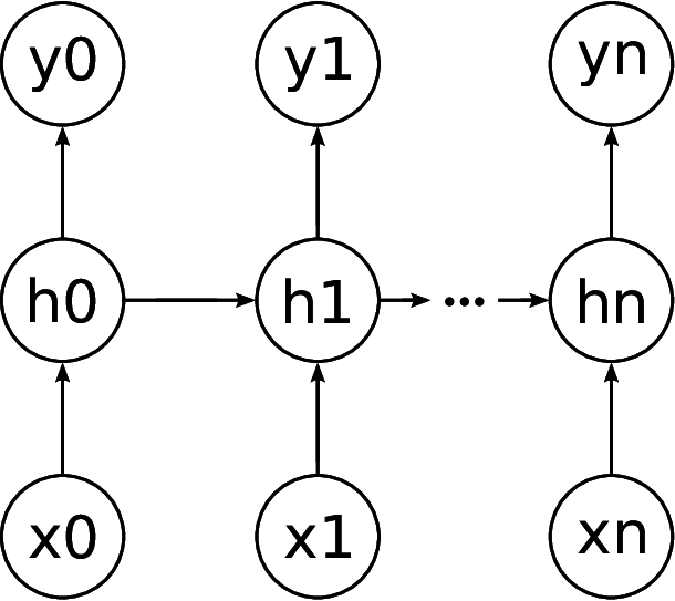
Fig. 2 shows the principle of sequence learning in an unrolled, or unfolded representation of the network over time. The input sequence , starting with up to , where is the sequence length, forming the context window of the network. The hidden state vector represents an RNN layer of a given time step , denotes the same layer on the next time step, and the horizontal arrow implies the recurrent connection between them. The corresponding output sequence , i.e., to , delivers the predictions of the network for the associated class labels. In the sequence classification task of TAD, we consider the mapping of the input vectors to only the last output vector . By assuming knowledge of the desired output, supervised learning of the neural networks is performed. The Backpropagation (BP) algorithm serves as a learning algorithm for FNNs and Backpropagation Through Time (BPTT) is used for training RNNs [25].
2.3 Network types
For exploiting the temporal dependencies among the feature vectors according to (6) for the TAD task, we consider three types of neural networks with memory, namely plain RNNs [25], (LSTMs) [26], and Gated Recurrent Units (GRUs) [27], and compare them to the memoryless FNNs [24]. The hidden state of the feed-forward layer is calculated as
| (7) |
with the weight matrix , the bias vector , and the nonlinear activation function . (7) is also referred to as gate, if it is employing a sigmoid function [26]. In the following, for both FNNs and RNNs the function is chosen to be the hyperbolic tangent function [24]. As opposed to memoryless FNNs, the group of RNNs considers the temporal dependencies of subsequent feature vectors by introducing recurrent connections to the previous time steps. The hidden state vector of a plain RNN is calculated as
| (8) |
with the previous hidden state vector weighted by the matrix . The inability of plain RNNs to model long-time dependencies initially motivated the use of LSTMs, proposed by [26], who introduced a memory unit, called cell state. This cell state is accessed by gate units, limiting the effect of vanishing gradients [28]. GRUs were introduced to reduce the complexity of LSTMs while maintaining a similar expressive power, by dropping the memory unit and operating with gate units directly on the hidden state vector . For a detailed description of the hidden state vector of an LSTM see [26], and for an GRU consider [27].
3 Experiments
We evaluated the proposed method in scenarios with up to five simultaneously active speech sources in reverberant environments for detecting time intervals, where the SINR exceeds a threshold of 10 dB, which is deemed relevant for practical applications [29].
3.1 Implementation and scenarios

| Performance | Complexity | |||||||
|---|---|---|---|---|---|---|---|---|
| Network type | ACC | AUC | MCC | / | RRT | RTT | ||
| FNN (nos) | 0.801 | 0.906 | 0.539 | 32 | 6 | 5634 / 712 | 1.785 | 1.188 |
| FNN (smo) | 0.870 | 0.950 | 0.662 | 32 | 2 | 1410 / 712 | 1 | 1 |
| FNN (seq) | 0.889 | 0.950 | 0.700 | 32 | 6 | 10498 / 2308 | 1.0955 | 1.074 |
| RNN | 0.905 | 0.961 | 0.721 | 16 | 2 | 994 / 1545 | 14.021 | 9.221 |
| LSTM | 0.917 | 0.961 | 0.732 | 32 | 1 | 5474 / 7403 | 36.638 | 22.609 |
| GRU | 0.904 | 0.960 | 0.710 | 32 | 4 | 22850 / 5408 | 26.969 | 11.897 |
For training the different network models and parameter sets, a software framework was implemented in Python, largely based on the library ‘Lasagne’ [30], which uses Compute Unified Device Architecture (CUDA) [31], performing the training using Stochastic Gradient Descent (SGD) [32], an Averaged Cross-Entropy (ACE) cost function, and a softmax output layer [25]. For regularization, dropout [33] is employed for FNNs and synaptic noise [34] for RNNs. To keep the search space for the network parameters low, the number of hidden layers is varied from to , and the number of neurons per layer is chosen between to in powers of two, which leads to a total of different configurations. A batch of training data comprises sequences, with each sequence consisting of feature vectors. The feature vector is computed from the observed signals every millisecond according to (6). The dataset consists of recordings of a desired target speaker, up to simultaneously active interferers, and babble noise in the background. The levels of targets and interferers are chosen to be equal and by varying the number of interferers different SINRs are obtained from the recordings, with a background noise level at -10 dB relative to a speech source. The target and interferer positions are static, and varied in an angular range between -135 ∘ and +135 ∘. The speech sources were recorded at a distance of 1 m in a living room-like environment at a sampling frequency of . The scenarios are split into a set of acoustic scenes of length 20 s (resulting in a total of labeled feature vectors) for training and validation, and acoustic scenes of length 10 s (resulting in a total of labeled feature vectors) for testing purposes. The ground truth for the target activity was defined by calculating the instantaneous SINR (with knowledge of the individual target source and interferer components) and applying a threshold of 10 dB, denoted as ‘10 dB-dataset’. This leads to binary output values, which are used for supervised learning. Fig. 3 shows the SINR distribution of the training data. The inequality in class labels is afterwards balanced by upsampling the minor class until equality in the number of class labels is reached. The threshold of 10 dB is chosen as a typical value for real-world requirements, as, e.g., Least Mean Squares (LMS)-type algorithms need a sufficiently high SINR for convergence [29].
3.2 Results
Six different network types are compared by their performance as well as their complexity in Tab. 1. For each network type, the configuration (defined by the number of neurons per layer and the number of layers ) has been chosen in terms of Matthew’s Correlation Coefficient (MCC) [35] on the validation set of the 10 dB-dataset. While MCC and Area Under Curve (AUC) [35] of a receiver operator characteristics deliver a viable measure when applied to unbalanced data, the Accuracy (ACC) measure [35], although commonly used, produces results of limited value. The ratio indicates the relative complexity of the chosen network compared to all other considered configurations. ‘FNN (nos)’ and ‘FNN (smo)’ are examples for instantaneous learning, where a single feature vector is classified by an FNN, exhibiting the lowest number of parameters on average. ‘FNN (smo)’ uses a recursively averaged feature vector , given by with , whereas ‘FNN (nos)’ uses the original feature vector (). ‘FNN (seq)’, ‘RNN’, ‘LSTM’ and ‘GRU’ are examples of sequence learning approaches. ‘FNN (seq)’ employs an FNN on a concatenation of a sequence of feature vectors to , which are introducing roughly times more weights in the first layer than ‘FNN (nos)’, where is the sequence length chosen to . In addition, the last three setups represent the group of RNNs. By additional recurrent connections, the plain RNN, denoted as ‘RNN’, is only about twice as complex as an ‘FNN (nos)’ on average, although performing sequence learning. By introducing gate units to control the information flow inside a neuron, ‘LSTM’ and ‘GRU’ are the most demanding setups regarding the number of parameters. Tab. 1 indicates that by recursively averaging, a significant performance gain of ‘FNN (smo)’ over ‘FNN (nos)’ is observable, confirming the benefit of incorporating averaged feature vectors into the classification. While ‘FNN (seq)’ outperforms the other FNNs due to its larger number of inputs and, accordingly the larger number of parameters, all RNNs outperform all considered feed-forward networks. Especially, the plain RNN requires roughly times less parameters compared to ‘FNN (seq)’, but delivers a better performance at the expense of an increased testing time. The recurrent nature of the group of RNNs indicate that they have learned the temporal evolution of the feature vectors through their feed-back connections. LSTMs and GRUs are not able to benefit from their long-term memory, which may be due to the nonstationarity of speech signals. While the three recurrent network types perform similarly well for TAD, the plain RNN shows the lowest number of parameters, which renders it the model of choice, especially for embedded applications demanding for low complexity.
4 Conclusion
In this paper, a set of TAD features is used at the input of a neural network detecting the activity of a desired speaker. As main innovation with respect to previous work, we propose to employ recursive layers in the neural network performing efficient TAD for embedded acoustic devices. In the experimental part using a multitude of challenging acoustic scenarios and comparing six different network types, we illustrate that RNNs outperform FNNs, pointing at the plain RNN as the structure of choice, due to the lowest number of trainable parameters involved. Future work will include additional features to further improve the characterization of the scenarios.
References
- [1] J. Ramírez, J. C. Segura, C. Benítez, A. De la Torre, and A. Rubio, “An effective subband OSF-based VAD with noise reduction for robust speech recognition,” IEEE Trans. Speech Audio Process., vol. 13, no. 6, pp. 1119–1129, 2005.
- [2] S. Gannot, D. Burshtein, and E. Weinstein, “Signal enhancement using beamforming and nonstationarity with applications to speech,” IEEE Trans. Signal Process., vol. 49, no. 8, pp. 1614–1626, 2001.
- [3] H. Barfuss, C. Huemmer, G. Lamani, A. Schwarz, and Kellermann, “HRTF-based robust least-squares frequency-invariant beamforming,” Proc. IEEE WASPAA, pp. 1–5, October 2015.
- [4] E. Hadad, S. Doclo, and S. Gannot, “The binaural LCMV beamformer and its performance analysis,” IEEE/ACM Trans. Audio, Speech, Language Process., vol. 24, no. 3, pp. 543–558, 2016.
- [5] S. Graf, T. Herbig, M. Buck, and G. Schmidt, “Improved performance measures for voice activity detection,” in Proc. ITG Conf. Speech Communication, pp. 1–4, VDE, 2014.
- [6] S. Graf, T. Herbig, M. Buck, and G. Schmidt, “Features for voice activity detection: a comparative analysis,” EURASIP J. Advances Signal Process., vol. 2015, no. 1, pp. 1–15, 2015.
- [7] H. Lee and D. Yook, “Space-time voice activity detection,” IEEE Trans. Consumer Electronics, vol. 55, no. 3, pp. 1471–1476, 2009.
- [8] M. J. Taghizadeh, P. N. Garner, H. Bourlard, H. R. Abutalebi, and A. Asaei, “An integrated framework for multi-channel multi-source localization and voice activity detection,” in Proc. IEEE Joint Workshop HSCMA, pp. 92–97, 2011.
- [9] Y. Denda, T. Nishiura, and Y. Yamashita, “Robust talker direction estimation based on weighted CSP analysis and maximum likelihood estimation,” IEICE Trans. Information and Systems, vol. 89, no. 3, pp. 1050–1057, 2006.
- [10] Y. Denda, T. Tanaka, M. Nakayama, T. Nishiura, and Y. Yamashita, “Noise-robust hands-free voice activity detection with adaptive zero crossing detection using talker direction estimation,” in Proc. Annual Conf. Interspeech, pp. 222–225, 2007.
- [11] R. Le Bouquin-Jeannès and G. Faucon, “Study of a voice activity detector and its influence on a noise reduction system,” Speech Communication, vol. 16, no. 3, pp. 245–254, 1995.
- [12] W. Herbordt, H. Buchner, and W. Kellermann, “An acoustic human-machine front-end for multimedia applications,” EURASIP J. Applied Signal Process., pp. 21–31, 2003.
- [13] T. Yu and J. H. Hansen, “An efficient microphone array based voice activity detector for driver’s speech in noise and music rich in-vehicle environments,” in Proc. IEEE ICASSP, pp. 2834–2837, IEEE, 2010.
- [14] S. Srinivasan and K. Janse, “Spatial audio activity detection for hearing aids,” in Proc. IEEE ICASSP, pp. 4021–4024, IEEE, 2008.
- [15] H.-D. Kim, J. Kim, K. Komatani, T. Ogata, and H. G. Okuno, “Target speech detection and separation for humanoid robots in sparse dialogue with noisy home environments,” in Proc. IEEE/RSJ Int. Conf. IROS, pp. 1705–1711, IEEE, 2008.
- [16] M. Taseska and E. A. Habets, “Minimum Bayes risk signal detection for speech enhancement based on a narrowband DOA model,” in Proc. IEEE ICASSP, pp. 539–543, IEEE, 2015.
- [17] Q. Wang, J. Du, X. Bao, Z.-R. Wang, L.-R. Dai, and C.-H. Lee, “A universal VAD based on jointly trained deep neural networks,” in Proc. Annual Conf. Interspeech, pp. 2282–2286, 2015.
- [18] X.-L. Zhang and D. Wang, “Boosting contextual information for deep neural network based voice activity detection,” IEEE/ACM Trans. Audio, Speech, Language Process., vol. 24, no. 2, pp. 252–264, 2016.
- [19] N. Moritz, J. Drefs, H. Baumgartner, and J. Rennies, “Sprachaktivitätserkennung basierend auf Deep Neural Networks für Anwendungen in Film und Fernsehen,” pp. 960–963, DAGA, March 2016.
- [20] S. Meier and W. Kellermann, “Artificial neural network-based feature combination for spatial voice activity detection,” in Proc. Annual Conf. Interspeech, September 2016.
- [21] S. Meier and W. Kellermann, “Relative impulse response estimation during doubletalk with an artificial neural network-based step size control,” in Proc. IWAENC, September 2016.
- [22] M. W. Hoffman, L. Zhao, and D. Khataniar, “GSC-based spatial voice activity detection for enhanced speech coding in the presence of competing speech,” IEEE Trans. Speech Audio Process., vol. 9, no. 2, pp. 175–179, 2001.
- [23] G. Elko and A.-T. N. Pong, “A simple adaptive first-order differential microphone,” in Proc. IEEE WASPAA, pp. 169–172, 1995.
- [24] C. M. Bishop, Neural Networks For Pattern Recognition. Clarendon Press, 1996.
- [25] A. Graves, Supervised sequence labelling. Springer, 2012.
- [26] S. Hochreiter and J. Schmidhuber, “Long short-term memory,” Neural computation, vol. 9, no. 8, pp. 1735–1780, 1997.
- [27] K. Cho, B. Van Merriënboer, C. Gulcehre, D. Bahdanau, F. Bougares, H. Schwenk, and Y. Bengio, “Learning phrase representations using RNN encoder-decoder for statistical machine translation,” arXiv preprint arXiv:1406.1078, 2014.
- [28] S. Hochreiter, “The vanishing gradient problem during learning recurrent neural nets and problem solutions,” International Journal of Uncertainty, Fuzziness and Knowledge-Based Systems, vol. 6, no. 02, pp. 107–116, 1998.
- [29] S. Haykin et al., “Adaptive filtering theory,” Englewood Cliffs, NJ: Prentice-Hall, 1996.
- [30] E. Battenberg, S. Dieleman, D. Nouri, E. Olson, A. van den Oord, C. Raffel, J. Schlüter, and S. Sonderby, “Lasagne: First release..” http://dx.doi.org/10.5281/zenodo.27878, Aug. 2015. Retrieved on 2016-04-18.
- [31] J. Nickolls, I. Buck, M. Garland, and K. Skadron, “Scalable parallel programming with CUDA,” Queue, vol. 6, no. 2, pp. 40–53, 2008.
- [32] D. Kingma and J. Ba, “Adam: A method for stochastic optimization,” arXiv preprint arXiv:1412.6980, 2014.
- [33] N. Srivastava, G. Hinton, A. Krizhevsky, I. Sutskever, and R. Salakhutdinov, “Dropout: A simple way to prevent neural networks from overfitting,” Journal Machine Learning Research, vol. 15, no. 1, pp. 1929–1958, 2014.
- [34] K.-C. Jim, C. L. Giles, and B. G. Horne, “An analysis of noise in recurrent neural networks: convergence and generalization,” IEEE Trans. Neural Netw., vol. 7, no. 6, pp. 1424–1438, 1996.
- [35] Y. Fang, X. Wang, E. K. Michaelis, and J. Fang, “Classifying aging genes into DNA repair or non-DNA repair-related categories,” International Conference Intelligent Computing, pp. 20–29, 2013.