The Effects of Magnetic Fields on the Dynamics of Radiation Pressure Dominated Massive Star Envelopes
Abstract
We use three dimensional radiation magneto-hydrodynamic simulations to study the effects of magnetic fields on the energy transport and structure of radiation pressure dominated main sequence massive star envelopes at the region of the iron opacity peak. We focus on the regime where the local thermal timescale is shorter than the dynamical timescale, corresponding to inefficient convective energy transport. We begin with initially weak magnetic fields relative to the thermal pressure, from in differing geometries. The unstable density inversion amplifies the magnetic field, increasing the magnetic energy density to values close to equipartition with the turbulent kinetic energy density. By providing pressure support, the magnetic field’s presence significantly increases the density fluctuations in the turbulent envelope, thereby enhancing the radiative energy transport by allowing photons to diffuse out through low density regions. Magnetic buoyancy brings small scale magnetic fields to the photosphere and increases the vertical energy transport with the energy advection velocity proportional to the Alfvén velocity, although in all cases we study photon diffusion still dominates the energy transport. The increased radiative and advective energy transport causes the stellar envelope to shrink by several scale heights. We also find larger turbulent velocity fluctuations compared to the purely hydrodynamic case, reaching at the stellar photosphere. The photosphere also shows vertical oscillations with similar averaged velocities and periods of a few hours. The increased turbulent velocity and oscillations will have strong impacts on the line broadening and periodic signals in massive stars.
Subject headings
stars: massive — (magnetohydrodynamics:) MHD — methods: numerical — radiative transferI. Introduction
Magnetic fields in the range to have been observed at the surface of 5-10% of O-type stars based on high-resolution, sensitive spectropolarimeters [14, 52, 53]. These fields are mostly dipolar and do not show rapid evolution, or any systematic correlations with stellar properties such as mass or rotation [29, 14, 30, 53]. One limitation of Zeeman spectro-polarimetry applied to unresolved stars, is that it is only sensitive to the mean component of the magnetic field, making the technique essentially blind to small scale fields below a certain amplitude [43, 27]. There exists indirect evidence that magnetic fields at the surface of massive stars could be much more common than revealed by current spectro-polarimetric observations, and could explain ubiquitous phenomena such as line profile variability [15] and discrete absorption components in UV spectra [26, 12].
Dynamo action in the rotating radiative regions of these stars has been suggested on theoretical grounds [46, 34], and equipartition magnetic fields could be generated by dynamo action in the sub-surface convective regions of massive stars [11, 9, 10]. During the main sequence, the most prominent sub-surface convective regions are located around the iron opacity peak, at temperatures K [32, 11, 39], where the opacity is enhanced by a factor of few compared with the electron scattering value and causes the local radiation acceleration to be larger than the gravitational acceleration. In this situation, analytical calculations and one dimensional stellar evolution models predict the development of a density inversion [25, 39].
[21] carried out the first three dimensional radiation hydrodynamic simulations around this region, showing that this density inversion is convectively unstable. When the iron opacity peak is close to the surface, where the optical depth per pressure scale height is smaller than , the ratio between the speed of light and the isothermal sound speed, convection is inefficient. The density inversion is not completely erased and, even when the envelope experiences strong density fluctuations and vertical oscillations, it still persists in a time averaged sense. In this paper we study how these results are affected by the presence of magnetic fields.
Magnetic fields are also interesting because they provide the opportunity for other instabilities to develop in the stellar envelope, even in the absence of rotation. One example is the photon bubble instability [3, 17], an overstability where the motion of the gas along the magnetic field lines is amplified by the radiation flux, leading to growing, propagating density variations [7]. Analytic work and numerical experiments [5, 51, 22] show that the photon bubble instability can result in shock trains propagating through the envelope.
Convection is also expected to be affected by the presence of a magnetic field, as the magnetic pressure for a 1 kG magnetic field is already comparable to the thermal pressure at the iron opacity peak. The standard convective instability associated with the iron opacity peak can turn into the interchange mode of the Parker instability, and the undulatory Parker instability also becomes possible if the magnetic energy density decreases outward [36, 18, 1].
The goal of this paper is to study the structure and the energy transport in radiation pressure dominated massive star envelopes, based on self-consistent three-dimensional (3D) radiation magneto-hydrodynamic simulations. In Section II, we describe the numerical method we use, which is a direct extension of the radiation hydrodynamic algorithm used in [21] including magnetic fields. The simulation setup and parameters we choose are also given in Section II. The main results are summarized in Sections III and IV. Implications of the simulation results for stellar evolution models and observations are given in Section V.
II. Numerical Method
II.1. Equations
Following [21], we model plane parallel massive star envelopes in cartesian coordinates with unit vectors by solving the following radiation magnetohydrodynamic (MHD) equations [22, e.g.,]
| (1) |
where the radiation source terms are
| (2) | |||||
Here are the gas density, pressure, flow velocity and speed of light respectively while is the sum of gas pressure and magnetic pressure. Notice that the unit of magnetic field is chosen such that magnetic permeability is . The total gas energy density is , where is the internal gas energy density with a constant adiabatic index . The gas pressure is , where is Boltzmann’s constant and is the mean molecular weight for nearly fully ionized gas with proton mass . The radiation constant is erg cm-3 K-4, while are the radiation energy density and flux. The Rosseland mean absorption and scattering opacities are denoted by and , while and are the Planck and energy mean absorption opacities. We use a variable Eddington tensor (VET), which is calculated by solving the time-independent radiation transfer equation based on the short-characteristic method [13], to relate the radiation pressure with the radiation energy density such that the radiation moment equations are closed. We solve these equations using the same radiation MHD code Athena as in [21] with the MHD module turned on. The code is described and tested in [22] with additional improvements described in [23].
II.2. Model Parameters
[21] show that the important parameters to distinguish different regimes of convection are optical depth per pressure scale height at the iron opacity peak , as well as the ratio between the speed of light and isothermal sound speed . When as in the post main sequence giant stars, convection is efficient and close to the adiabatic convection regime with adiabatic index . When as in the main sequence massive stars, convection is inefficient because of rapid diffusion and porosity effects become significant. This is also the regime where accurate radiation transfer is crucial. Because the iron opacity peak is closer to the surface in this case, the magnetic field amplified by convection could easily reach the photosphere and affect the observable properties of massive stars.
Therefore we focus on the parameter regime corresponding to the run StarTop shown in Table 1 of [21] with and . The model parameters are taken from a MESA[38, 39, 40] calculation of a main sequence star. The simulation box is located at radius with a constant gravitational acceleration cm/s2 and a constant radiation flux erg/(cm2 s) applied at the bottom of the simulation box, which are the same as in StarTop. Horizontal and vertical sizes of the simulation box are and with resolution and , where cm is the fiducial pressure scale height. The fiducial density, temperature, velocity, gas pressure and time units are g/cm3, K, cm/s, dyn/cm3 and s. These fiducial units are summarized in Table 1. The initial gas and radiation pressure at the iron opacity peak is and . Compared with StarTop, the horizontal box size is increased by with a comparable resolution.
The total Rosseland mean opacity in the simulation is calculated based on opacity tables taken from MESAwith assumed metallicity and hydrogen fraction (Figure 2 of Jiang et al. 21). We assume a constant electron scattering opacity cm2/g and absorption opacity is simply calculated as . The Planck and energy mean absorption opacities are taken to be the same as .
| Variables/Units | Values |
|---|---|
| / cm | |
| / g cm-3 | |
| / K | |
| / cm s-1 | |
| / dyn cm-3 | |
| / s |
II.3. Simulation Setup
Initial vertical profiles of the gas and radiation quantities are constructed in the same way as described in Section 3.3 of [21], which are calculated based on equations of hydrostatic and thermal equilibrium. We add a uniform vertical () and horizontal magnetic field () through the whole simulation box, which does not affect the initial conditions of other quantities. Values of magnetic field strengths and configurations we have explored are listed in Table 2. For simulations StarB1, StarB2 and StarB3, the magnetic field is inclined by with respect to the horizontal plane but they have different magnetic field strengths. Simulation StarB4 has the same as StarB3 but is increased by a factor of 5 compared with StarB3. Therefore, the magnetic field has an initial inclination angle with respect to the horizontal plane.
| Variables/Units | StarB1 | StarB2 | StarB3 | StarB4 |
|---|---|---|---|---|
| 60 | 191 | 382 | 382 | |
| 121 | 382 | 764 | 3819 | |
| 11373 | 1137 | 284 | 284 | |
| 800 | 80 | 20 | 20 |
- •
Note: The gas pressure and radiation pressure are the initial values at the iron opacity peak. The vertical and horizontal magnetic field components (with magnetic pressure ) and are the initial values and only is conserved during the simulations. Notice that magnetic field unit is converted to Gauss here from the code unit by matching the dimensionless ratio .
We use the same boundary conditions for the gas and radiation quantities as described in section 3.3 of [21], namely, reflecting boundary condition at the bottom and outflow boundary condition at the top. For magnetic field at the bottom boundary, the vertical component is copied from the last active zones to the ghost zones while the horizontal components and are copied with the opposite sign. We have also tried to just copy and from the last active zones to the ghost zones, which does not make any noticeable difference. At the top boundary, the vertical component is copied from the last active zones to the ghost zones and the horizontal components and are also copied when the vertical component of flow velocity points outward. When points inward, and are set to be zero in the ghost zones to avoid magnetic field being carried into the simulation domain from the top boundary. In this setup, the volume integrated is a conserved quantity while the volume integrated and can change. In particular, and can escape through the open top boundary while cannot.
III. Results
In this section, we describe how the initial development of convection and the final turbulent structures of the envelope are modified by different magnetic field strengths and configurations. For any quantity , we will use to represent the horizontal averaged value for each height .
III.1. Linear Growth Phase of the Instabilities

As in the hydro case, there is a density inversion around in the initial hydrostatic envelope at the iron opacity peak where the local radiation acceleration is larger than gravitational acceleration. The initial profile we construct is actually pretty similar to the 1D MESAprofile in this regime, as convection is inefficient to transport energy. In our 3D simulations, the density inversion is unstable to convection, resulting in the development of turbulence after . In simulation StarB1 when the initial magnetic pressure is much smaller than both the gas and radiation pressure, the initial growth rate and the dominant wavelength of the convection are very similar to the hydro case shown in [21]. For simulation StarB3 when the initial total magnetic pressure is comparable to the gas pressure at the iron opacity peak, it only takes to completely destabilize the density inversion, compared to in StarB1. The fastest growing mode is also modified by the presence of a magnetic field. Figure 16 of [21] shows that during the linear growth phase of convection, the long wavelength mode dominates and it is roughly symmetric with respect to and directions. This is also true for run StarB1 when the initial magnetic field is weak. However, during the linear growth phase of StarB3, as shown in the left panel of Figure 1, the magnetic field breaks the symmetry. Short wavelength modes dominate along the direction perpendicular to the magnetic field, and are the result of Parker instability. For the run StarB4 when is increased such that the angle between the magnetic field and the horizontal direction is decreased, we see both the instability associated with the density inversion as well as shock trains in the envelope as shown in the right panel of Figure 1. This is very similar to the nonlinear outcome of the photon bubble instability [5, 51]. The shock fronts are inclined by an angle of roughly with respect to the direction of gravity.
The properties of these instabilities compare well with linear theory. For the photon bubble instability, the maximum growth rate is achieved for wavelengths shorter than [8], where is the gas sound speed. However, this very short length scale is unresolved by the simulation, and is in fact optically thin so the diffusive transport of photons that drives the instability does not even apply at these wavelengths. Longer wavelength growth rates can be estimated by neglecting the sound speed in the gas alone [17, 8], giving a dispersion relation for the angular frequency of the mode
| (3) |
Here is the wavevector of the wave and is a unit vector in the direction of the magnetic field. The quantity is the logarithmic derivative of the Rosseland mean opacity with respect to density at fixed temperature, and is approximately 0.1 throughout our simulation, and can therefore be neglected. This then gives a photon bubble growth rate that depends only on wavelength and the direction of propagation, and is almost independent of height. For StarB4, the magnetic field is inclined by to the horizontal, and this gives a maximum growth rate for wavefronts that are inclined by to the vertical, exactly as we observe in the simulations. Inclining the magnetic field further away from the horizontal reduces the maximum growth rate, which may explain why there are no obvious shock trains in the other simulations.
In order to estimate the linear growth rates in the simulations, we perform a Fourier transform of density at heights and for each snapshots. Histories of the binned 1D power spectrums for two different wave numbers are shown in Figure 2 at (left panel) and (right panel). The growth rates are larger at higher height because the horizontal magnetic field can leave the simulation box from the top boundary, which results in a larger magnetic pressure gradient at . The maximum photon bubble growth rate for a wavelength equal to is , and this compares favorably to the measured growth rate of at . At , the medium is actually supported by magnetic pressure gradients, and this is Parker unstable. While photon bubbles and Parker instabilities arise from the same underlying mode [50], Parker dominates for short horizontal wavelengths that are perpendicular to the magnetic field, and this is exactly what we see in the simulations in this region. When photons diffuse rapidly and the gas pressure is negligible, as is the case here, the maximum instability growth rate is , where is the local magnetic pressure scale height [50]. This gives a peak growth rate of approximately peaking in the region , independent of wavelength, in rough agreement with the growth rates we find in this region. Notice that these growth rates are much larger than the growth rate of hydrodynamic convection, which is for wavelength . The smaller growth rates for the short wavelength modes at both heights in Figure 2 are probably because of extra numerical dissipation, which we also observe in the run StarTop [21].
III.2. Steady State Turbulent Structures

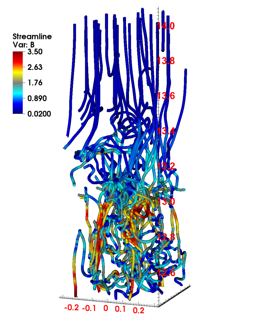
Although the shock trains caused by the photon bubble instability show up in run StarB4 but not StarB3, the final turbulent structures of the envelopes in the two runs are very similar. Snapshots of density for the two runs after the initial development of the instabilities are shown in Figure 3. The entire envelopes are turbulent due to convection, while the shock trains from the photon bubble instability are hardly noticeable in StarB4. The Parker instability has grown to completely dominate the turbulent state, and in fact the magnetic field geometry has completely changed from its initial configuration. As shown in Figure 4, the magnetic field is dominated by the vertical component, as the horizontal component has buoyantly left the simulation domain. This vertical field configuration is also less able to support the weight of high density regions within photon bubble shock trains (cf. the right hand panel of Figure 1 of Turner et al. 51). Figure 4 also shows that a small scale turbulent magnetic field dominates in the iron opacity region. Above , only the vertical magnetic field survives.


The whole histories of the horizontally averaged vertical profiles of , , and for simulations StarB1 and StarB3 are shown in Figure 5. After the onset of turbulence, the stellar envelope undergoes regular vertical oscillations as shown in Figure 5, which is also observed in the pure hydrodynamic simulation. The oscillation amplitude increases with increasing magnetic field strength, which causes larger temporal variability at the photosphere. Vertical advection flux oscillates with the envelope. However, there is always more outward advection flux than inward advection flux, which results in net positive advection flux.
It is clear from Figure 5 that the averaged positions of the oscillated envelopes and the oscillation amplitude are different with different magnetic field strengths. The time and horizontally averaged vertical profiles of density, opacity, entropy and radiation accelerations during the oscillation periods for the runs StarTop, StarB1, StarB2, StarB3 and StarB4 are shown in Figure 6. Compared with the hydro case, the whole envelopes shrink and the iron opacity peaks move from as in StarTop to in StarB1, in StarB2, in StarB3. The change of iron opacity peak locations from StarTop to StarB3 corresponds to . The three runs StarB1, StarB2, StarB3 also show that for the same initial magnetic field configuration, larger initial magnetic fields strengths correspond to larger envelope shrinking. The field geometry does not seem to play an important role for the final envelope structure, as shown by the fact that StarB3 and StarB4 (same initial amplitude, different geometry) reach very similar vertical structures, particularly in the regions around and below the iron opacity peaks. In the regions above the iron opacity peak, the magnetic field plays a significant role in providing support against gravity, particularly in runs StarB3 and StarB4, which causes the density to drop slowly with height. Stronger initial horizontal magnetic field causes stronger magnetic pressure support in this region. This is mainly because most of the initial horizontal magnetic field has moved to the top part of the box due to buoyancy. In the steady state, the buoyantly rising magnetic field from the convective region is balanced by the magnetic flux loss through the top of the simulation domain.
When the iron opacity peak is moved to the higher density region, the maximum opacity is increased as shown in the panel (c) of Figure 6. For the same radiation flux, the radiation acceleration is also increased as shown in the panel (d) of Figure 6. However, the density weighted radiation acceleration is actually smaller with stronger magnetic field. Therefore, the remaining density inversions in the time averaged structures are weaker with flatter entropy profiles as shown in panel (b) of the same Figure. This will be explained in Section IV.1.
The time averaged vertical profiles of radiation energy density , gas internal energy density , total magnetic energy density as well as the magnetic energy density associated with the horizontally averaged mean vertical component of magnetic field are shown in Figure 7. Because vertical magnetic flux is conserved, is the same as the initial vertical magnetic field . The magnetic energy density includes contributions from the turbulent magnetic field as well as the horizontally averaged mean magnetic field. In the convective region near the iron opacity peak, the turbulent component associated with the convection dominates as is much larger than . Above the iron opacity peak, gets close to . This is also consistent with the magnetic field streamlines shown in Figure 4. In steady state, the vertical component of radiation pressure dominates everywhere for the four runs, although in the regions above the iron opacity peak, the magnetic pressure gets close to the radiation pressure in StarB3 and StarB4.
The kinetic energy densities in the steady state between the run StarTop without magnetic field and the four runs with magnetic field are compared in Figure 8. The peak value of in StarB3 is increased by a factor of 3 compared with the value in StarTop. Despite the large differences of the initial magnetic field strengths, the kinetic energy density in the turbulent state is only increased by from StarB1 to StarB3. The ratios between the magnetic and kinetic energy densities in the turbulent state only vary from 0.2 to 0.6 in the three runs StarB1, StarB2 and StarB3, as shown in the bottom panel of Figure 8. This suggests that convection is driving a reasonably efficient small-scale magnetic dynamo. The run StarB4 reaches similar kinetic energy density and vertical component of magnetic energy density as in the run StarB3, although the initial horizontal magnetic field is times stronger in StarB4 compared with StarB3. This also suggests that the photon bubble instability that shows up in the run StarB4 (Figure 1) does not affect the vertical structures of the envelope (such as density, kinetic energy density, entropy) significantly compared with the run StarB3, although the two runs do have different ratios .
IV. Radiation Force and Energy Transport
IV.1. The Porosity Factor
The simulation StarTop is in the regime that the optical depth per pressure scale height is smaller than the critical value [21]. This is also true for all the MHD runs, even though the opacity peak is increased a little bit when the envelopes shrink. One important effect in this regime is that when photons go through the turbulent convective region in this regime, the radiation flux is stronger in the low density region [44, e.g.,]. This causes an anti-correlation between density and radiation flux fluctuations at each height. The density weighted radiation acceleration (equation 14 of Jiang et al. 21) can be decomposed as
| (4) | |||||
Because of the existence of the anti-correlation, this is smaller than the volume averaged radiation acceleration . The porosity factor
| (5) |
for the hydro run StarTop and the four MHD runs are shown in the top panel of Figure 9. Although magnetic pressure is small compared with the radiation pressure, it increases the porosity factor significantly compared with the hydro case. The stronger the initial magnetic field strength, the larger is the porosity factor. In the run StarB3, F reaches at the iron opacity peak. It is also not sensitive to the initial horizontal magnetic field, as the two runs StarB3 and StarB4 have very similar F. This is also consistent with the fact that the two runs have very similar vertical structures. The increased porosity factor with magnetic field explains why the envelopes with magnetic field will shrink and in the MHD runs is actually smaller than the value in the hydro case, although the volume averaged radiation accelerations in the MHD runs are larger.
Magnetic field increases the porosity factor as it increases the density fluctuations, which is shown in the middle panel of Figure 9. The increase of from StarTop to StarB3 agrees pretty well with the change of F. At a given height, the low and high density regions should be roughly in pressure balance. In the hydro case, the gas pressure difference caused by the density fluctuations can only be balanced by the radiation pressure horizontally. But because of rapid diffusion, fluctuations of radiation pressure are small (Figure 20 of Jiang et al. 21), which limits the amount of density fluctuations that can be achieved. However, with magnetic field, magnetic pressure is larger in the low density regions, which can balance the gas pressure gradient. This is confirmed in the bottom panel of Figure 9, which shows strong anti-correlations between density and magnetic energy density fluctuations (negative ) for all the MHD runs. Here is the cross correlation coefficient between and normalized by their standard deviations at each height. This allows larger density fluctuations compared with the hydro case. Therefore, the anti-correlation between density and radiation flux as well as the porosity factor F are increased.
IV.2. Vertical Energy Transport
In the regime when , most of the energy is transported by the diffusive radiation flux while the advective radiation flux is negligible. This is because the photon diffusion time scale across the pressure scale height is smaller than the sound crossing time for the isothermal sound speed in this regime. However, with magnetic fields, magnetic buoyancy increases the vertical advection velocity and thus the advection flux, which is shown in the top panel of Figure 10. The ratio between the vertical advection flux and the total flux increases from in StarTop to in StarB3. Although the advection flux is increased with magnetic field, it is still a small fraction () of the total energy flux. Different vertical structures of the envelopes with magnetic field are not due to the change of advection flux. Instead, it is due to different porosity factors.
The larger the initial vertical magnetic field is, the stronger the advection flux. The vertical advection velocity also increases with increasing magnetic field for a given magnetic field configuration as shown in the middle panel of Figure 10. The effect of enhanced advection flux due to magnetic buoyancy is also observed in black hole accretion disk simulations with turbulence caused by magneto-rotational instability (MRI) [6, 24]. As shown in Figure 9 of [6], this can also be easily understood in terms of the larger density fluctuations due to magnetic field. The radiation energy density , density and vertical velocity at each height can be separated into the time and horizontally averaged mean values and the fluctuation components
| (6) |
Because there is no net mass flux,
| (7) |
Therefore, we have
| (8) |
The vertical energy advection velocity can then be calculated as
| (9) | |||||
As relative fluctuations of are much smaller than the relative fluctuations in in this rapid diffusion regime [21], the radiation advection flux is basically the mean vertical velocity multiplied by the horizontally averaged radiation energy density. That is why radiation advection flux increases with increasing density fluctuations. Comparing the two runs StarB3 and StarB4 shows that the vertical advection velocity does depend on the magnetic field configuration. Larger horizontal magnetic field actually decreases the vertical energy advection velocity.
Following [47] (see also MacGregor & Cassinelli 31 and Cantiello & Braithwaite 9), we show that when the vertical energy advection velocity (and thus density fluctuation) is dominated by magnetic buoyancy, it is proportional to the Alfvén velocity . Considering density fluctuations with typical radius , magnetic pressure inside the low density region balances the gas pressure inside the high density region with almost a constant temperature at each height due to rapid photon diffusion. The buoyancy force per unit length is , where is the gas pressure scale height. In steady state, the buoyancy force is balanced by the drag , where is the drag coefficient. Then the vertical velocity can be estimated as
| (10) |
The ratio between the vertical energy advection velocity and Alfvén velocity for the MHD runs are shown in the bottom panel of Figure 10. For runs StarB1, StarB2 and StarB3, which have the same initial magnetic field configuration, the ratios are pretty similar despite the large differences of magnetic field strength. The ratios peak at the location of the iron opacity peaks for each run. The coefficient decreases with distance from the iron opacity peak. It also depends on the magnetic field configuration as shown by the run StarB3 and StarB4. Its value is smaller with stronger horizontal magnetic field.
IV.3. Magnetic Fields in the Efficient Convection Regime
In the regime as in the run StarDeep studied by [21], the porosity factor F is (see panel d of Figure 7 in Jiang et al. 21), which means that the effective radiation acceleration is not reduced by the density and radiation flux fluctuations. With magnetic fields, the density fluctuations are expected to be larger, but as long as in the low density region is still much larger than , F is not going to be affected.
In the regime of efficient convection (), magnetic buoyancy will still increase the vertical advection velocity, but it cannot increase the advection flux significantly, as this is limited by the total available energy flux. However, magnetic buoyancy may result in different vertical structures compared to the case of efficient hydrodynamic convection. For example, we have shown that the advection flux caused by magnetic buoyancy is proportional to , which cannot be calculated based on the thermal entropy gradient as in the mixing length theory. Detailed comparisons between the magnetic buoyancy driven convection and mixing length theory, as well as the resulting stellar structures, will be the subjects of future investigation.
V. Discussions and Conclusions
We have extended the work of [21] by studying the effects of magnetic fields on the envelope structure and energy transport of main sequence massive stars at the location of the iron opacity peak. We focus on the regime so that the diffusion time scale is shorter than the local dynamical time scale and convection is inefficient. We found that the presence of magnetic fields with amplitude G-1 kG increases the density fluctuations in the turbulent envelope, resulting in a larger porosity factor and consequentially an enhanced transport of energy by the radiation field. The presence of magnetic buoyancy also increases the advection flux significantly, with the energy advection velocity proportional to the Alfvén velocity for a fixed magnetic field configuration. Both effects contribute to increasing the energy transport across the turbulent envelope compared to the pure hydrodynamic case, which causes the envelope to shrink by several scale heights.
V.1. Implications for 1D Stellar Evolution
Stellar evolution calculations adopt mixing length theory for calculating the energy transport in inefficient convective regions. In this regime, different assumptions for the mixing length result in large differences in the stellar radii of massive star models [28, see e.g. Fig. 20 in]. However, as discussed in e.g., Jiang et al. [21], mixing length theory is inadequate for treating the energy transport in radiation dominated stellar envelopes when convection is inefficient (), meaning that current stellar evolution calculations may provide inaccurate results. This is also true in the presence of magnetic fields. Because the entropy gradient is smaller in the MHD runs compared with the hydro run StarTop (Figure 6), if we adopt the same as in StarTop, the convective fluxes predicted by the mixing length theory for StarB1, StarB2 and StarB3 are much smaller than the corresponding value for StarTop. They are also significantly smaller than the advective flux we get from the simulations. In order to match the calculated fluxes with the mixing length theory at the iron opacity peaks, we need for StarB1, StarB2 and StarB3 respectively, which are much larger than the ratios between the correlation lengths and pressure scale height. Even if we can match the convective flux at the iron opacity peak, the convective flux drops quickly away from the iron opacity peaks in the mixing length theory and becomes much smaller than what we get from the simulations. To model inefficient convection correctly in 1D stellar evolution codes, two steps are required: 1) Calibrating the mixing length theory using 3D MHD calculations, and 2) Including the effect of porosity on the radiative energy transport.
V.2. Observational Consequences
Inefficient convection causes the development of supersonic turbulent velocities with respect to the isothermal sound speed. As a result, we find large density and velocity fluctuations in the simulated stellar envelopes. The vertical velocity fluctuations increase with the initial amplitude of the vertical component of the magnetic field. The average turbulent velocity reaches at the photosphere in our model with G (StarB3), which is about of the escape velocity. These fluctuations can impact the spectroscopic measurements of line profiles, potentially affecting both the microturbulence and macroturbulence parameters [11, 21]. Recent spectroscopic observations of a large sample of OB stars revealed a very interesting trend, with macroturbulent velocities increasing with stellar luminosity [45]. This has been tentatively attributed to the increasing turbulent pressure in the iron convection zone [20, 19], since turbulent pressure fluctuations may trigger high-order high-angular degree oscillations that can collectively mimic the effect of macroturbulence [2]. Despite capturing the relevant physics, our cartesian box calculations can not provide detailed predictions for the observed spectroscopic signature of radiation dominated envelopes of massive stars. Such predictions require global envelope calculations, which we will explore in future work.
Here we have studied the effects of magnetic fields up to values close to equipartition with thermal pressure at the location of the iron opacity peak ( kG). Magnetic fields with larger amplitude are expected to have a different impact on the convective properties, potentially decreasing the amount of turbulence in the outer stellar envelope. Such effects were discussed by Sundqvist et al. [49], who reported the observation of magnetic inhibition of photospheric macroturbulence in an O-star with a surface dipolar field of 20 kG. Interestingly, magnetic O-stars with smaller amplitude surface magnetic fields (implying sub-equipartition with thermal pressure at the location of the iron opacity peak) show normal macroturbulent velocities (20-60 ). This result strongly supports a causal link between the observed surface turbulence and the sub-surface convection associated with the iron opacity peak [11, 49, 20, 19].
It has been suggested that magnetic fields can be generated by dynamo action in the sub-surface convective regions [11, 10], and that they can reach the photosphere and affect the observable properties of massive stars [9]. Our calculations support these claims, showing that an initial magnetic field is efficiently amplified by turbulent motions around the iron opacity peak and rises buoyantly to reach the stellar photosphere (see Fig. 7). Possible impact of these buoyant magnetic fields includes photometric variability due to surface magnetic spots and/or prominences [9, 48], excess X-ray emission [16, 4, 54, 35, 37], as well as wind variability and clumping [41, 33].
While massive stars are rapid rotators, in this work we have not considered the effects of rotation. It is conceivable that the inclusion of rotation might impact the details of dynamo action in the turbulent convection around the iron opacity peak. Moreover, even in the radiative parts of the stellar envelope, differential rotation is expected to potentially trigger the Spruit-Tayler dynamo [46] or even the MRI [55, e.g.]. The interplay between these different dynamo-generated magnetic fields could be extremely important for angular momentum transport and internal mixing across massive star envelopes. These local calculations also do not include the possibility of mass loss, which may also change the structures in the iron opacity region [42]. The interplay between convection in this region and winds will be the focus of future global calculations of massive star envelopes.
Acknowledgements
Y.F.J thanks all members of the SPIDER network for helpful discussions. This work was supported by the computational resources provided by the NASA High-End Computing (HEC) Program through the NASA Advanced Supercomputing (NAS) Division at Ames Research Center; and the National Energy Research Scientific Computing Center, a DOE Office of Science User Facility supported by the Office of Science of the U.S. Department of Energy under Contract No. DE-AC02-05CH11231. This research is funded in part by the Gordon and Betty Moore Foundation through Grant GBMF5076 to L. B. and E. Q. and is supported in part by the National Science Foundation under NSF PHY-1125915 and by NASA under NNX14AB53G. EQ was also supported in part by a Simons Investigator Award from the Simons Foundation.
References
- [1] Acheson, D. J. 1979, Sol. Phys., 62, 23
- [2] Aerts, C., Puls, J., Godart, M., & Dupret, M.-A. 2009, A&A, 508, 409
- [3] Arons, J. 1992, ApJ, 388, 561
- [4] Babel, J., & Montmerle, T. 1997, ApJ, 485, L29
- [5] Begelman, M. C. 2001, ApJ, 551, 897
- [6] Blaes, O., Krolik, J. H., Hirose, S., & Shabaltas, N. 2011, ApJ, 733, 110
- [7] Blaes, O., & Socrates, A. 2001, ApJ, 553, 987
- [8] —. 2003, ApJ, 596, 509
- [9] Cantiello, M., & Braithwaite, J. 2011, A&A, 534, A140
- [10] Cantiello, M., Braithwaite, J., Brandenburg, A., et al. 2011, in IAU Symposium, Vol. 272, Active OB Stars: Structure, Evolution, Mass Loss, and Critical Limits, ed. C. Neiner, G. Wade, G. Meynet, & G. Peters, 32–37
- [11] Cantiello, M., Langer, N., Brott, I., et al. 2009, A&A, 499, 279
- [12] Cranmer, S. R., & Owocki, S. P. 1996, ApJ, 462, 469
- [13] Davis, S. W., Stone, J. M., & Jiang, Y.-F. 2012, ApJS, 199, 9
- [14] Donati, J.-F., & Landstreet, J. D. 2009, ARA&A, 47, 333
- [15] Fullerton, A. W., Gies, D. R., & Bolton, C. T. 1996, ApJS, 103, 475
- [16] Gagné, M., Caillault, J.-P., Stauffer, J. R., & Linsky, J. L. 1997, ApJ, 478, L87
- [17] Gammie, C. F. 1998, MNRAS, 297, 929
- [18] Gilman, P. A. 1970, ApJ, 162, 1019
- [19] Grassitelli, L., Fossati, L., Langer, N., et al. 2016, A&A, 593, A14
- [20] Grassitelli, L., Fossati, L., Simón-Diáz, S., et al. 2015, ApJ, 808, L31
- [21] Jiang, Y.-F., Cantiello, M., Bildsten, L., Quataert, E., & Blaes, O. 2015, ApJ, 813, 74
- [22] Jiang, Y.-F., Stone, J. M., & Davis, S. W. 2012, ApJS, 199, 14
- [23] —. 2013, ApJ, 767, 148
- [24] —. 2014, ApJ, 784, 169
- [25] Joss, P. C., Salpeter, E. E., & Ostriker, J. P. 1973, ApJ, 181, 429
- [26] Kaper, L., & Henrichs, H. F. 1994, Ap&SS, 221, 115
- [27] Kochukhov, O., & Sudnik, N. 2013, A&A, 554, A93
- [28] Köhler, K., Langer, N., de Koter, A., et al. 2015, A&A, 573, A71
- [29] Landstreet, J. D., & Mathys, G. 2000, A&A, 359, 213
- [30] Landstreet, J. D., Silaj, J., Andretta, V., et al. 2008, A&A, 481, 465
- [31] MacGregor, K. B., & Cassinelli, J. P. 2003, ApJ, 586, 480
- [32] Maeder, A., Georgy, C., & Meynet, G. 2008, A&A, 479, L37
- [33] Michaux, Y. J. L., Moffat, A. F. J., Chené, A.-N., & St-Louis, N. 2014, MNRAS, 440, 2
- [34] Mullan, D. J., & MacDonald, J. 2005, MNRAS, 356, 1139
- [35] Nazé, Y., Petit, V., Rinbrand, M., et al. 2014, ApJS, 215, 10
- [36] Newcomb, W. A. 1961, Physics of Fluids, 4, 391
- [37] Owocki, S. P., ud-Doula, A., Sundqvist, J. O., et al. 2016, MNRAS, 462, 3830
- [38] Paxton, B., Bildsten, L., Dotter, A., et al. 2011, ApJS, 192, 3
- [39] Paxton, B., Cantiello, M., Arras, P., et al. 2013, ApJS, 208, 4
- [40] Paxton, B., Marchant, P., Schwab, J., et al. 2015, ApJS, 220, 15
- [41] Puls, J., Markova, N., Scuderi, S., et al. 2006, A&A, 454, 625
- [42] Ro, S., & Matzner, C. D. 2016, ApJ, 821, 109
- [43] Schnerr, R. S., Henrichs, H. F., Neiner, C., et al. 2008, A&A, 483, 857
- [44] Shaviv, N. J. 1998, ApJ, 494, L193
- [45] Simón-Díaz, S., Godart, M., Castro, N., et al. 2016, arXiv:1608.05508
- [46] Spruit, H. C. 2002, A&A, 381, 923
- [47] Stella, L., & Rosner, R. 1984, ApJ, 277, 312
- [48] Sudnik, N. P., & Henrichs, H. F. 2016, A&A, 594, A56
- [49] Sundqvist, J. O., Petit, V., Owocki, S. P., et al. 2013, MNRAS, 433, 2497
- [50] Tao, T., & Blaes, O. 2011, ApJ, 742, 8
- [51] Turner, N. J., Blaes, O. M., Socrates, A., Begelman, M. C., & Davis, S. W. 2005, ApJ, 624, 267
- [52] Wade, G. A., Grunhut, J., Alecian, E., et al. 2014, in IAU Symposium, Vol. 302, IAU Symposium, 265–269
- [53] Wade, G. A., Neiner, C., Alecian, E., et al. 2016, MNRAS, 456, 2
- [54] Waldron, W. L., & Cassinelli, J. P. 2009, ApJ, 692, L76
- [55] Wheeler, J. C., Kagan, D., & Chatzopoulos, E. 2015, ApJ, 799, 85